HAL Id: hal-01320492
https://hal.archives-ouvertes.fr/hal-01320492
Submitted on 23 May 2016
HAL is a multi-disciplinary open access
archive for the deposit and dissemination of
sci-entific research documents, whether they are
pub-lished or not. The documents may come from
teaching and research institutions in France or
abroad, or from public or private research centers.
L’archive ouverte pluridisciplinaire HAL, est
destinée au dépôt et à la diffusion de documents
scientifiques de niveau recherche, publiés ou non,
émanant des établissements d’enseignement et de
recherche français ou étrangers, des laboratoires
publics ou privés.
Minimal time spiking in various ChR2-controlled neuron
models
Vincent Renault, Michèle Thieullen, Emmanuel Trélat
To cite this version:
Vincent Renault, Michèle Thieullen, Emmanuel Trélat.
Minimal time spiking in various
ChR2-controlled neuron models. Journal of Mathematical Biology, Springer Verlag (Germany), 2018, 76
(3), pp.567–608. �10.1007/s00285-017-1101-1�. �hal-01320492�
Minimal time spiking in various ChR2-controlled neuron
models
Vincent Renault, Michèle Thieullen
⇤, Emmanuel Trélat
†Abstract
We use conductance based neuron models and the mathematical modeling of Optogenetics to define controlled neuron models and we address the minimal time control of these affine systems for the first spike from equilibrium. We apply tools of geometric optimal control theory to study singular extremals and we implement a direct method to compute optimal controls. When the system is too large to theoretically investigate the existence of singular optimal controls, we observe numerically the optimal bang-bang controls.
Keywords. Conductance-based neuron models, optimal control, minimal time affine control, singular extremals, Optogenetics.
AMS Classification. 49J15. 93C15. 92C20.
Introduction
In this paper we investigate, theoretically and numerically, the minimal time control, via Optoge-netics, of some widely used finite-dimensional deterministic neuron models such as the Hodgkin-Huxley model ([16]), the Morris-Lecar model ([17]) and the FitzHugh-Nagumo model ([11]). Con-trol of neuron models has been addressed in the literature in different ways. One popular way to investigate this problem is to look at phase reductions of non-linear evolution systems, consisting in reducing the system of equations to a single first-order differential equation, with for essential goal numerical computations of the dynamic programming formulation of the problem ([5], [20]). Integrate-and-fire models, which are also a simplification of nonlinear sytems to single first-order linear differential equations, receiving stochastic inputs, have been studied in [10] in order to min-imize the variance of the membrane potential, arguably linked to the variance of the final time, while reaching a given membrane potential threshold in fixed time. Theses simplifications allow the authors to obtain a nice analytic expression for the optimal control. A stochastic integrate-and-fire models have also been used in [19] to find an optimal electrical stimulation to spike in a desired time, a problem close to ours, with numerical computation purposes.
All these studies were exclusively based on control via electrical stimulation. Optogenetics allows a control of excitable cells of a different nature. This recent and thriving technique is based on light stimulation ([7],[3],[8]). It has for cornerstone the genetical modification of excitable cells for them to express new ion channels whose opening and closing are triggered by the absorption of photons. In particular, it is able to target specific populations of neurons. Indeed, by designing viruses that will aim at these populations only, the light stimulation will have no effect on the other populations that do not express the new ion channels. This makes Optogenetics a noninvasive technique, in contrast to electrical stimulation that reaches a whole volume of tissue, regardless of the types of neurons that populate this volume. Furthermore, optical devices such as optic fibers and lasers allow to reach deeply embedded populations of neurons. It then provides Optogenetics
⇤Sorbonne Universités, UPMC Univ Paris 06, CNRS UMR 7599, Laboratoire de Probabilités et Modèles Aléa-toires, F-75005, Paris, France. email: [email protected], [email protected]
†Sorbonne Universités, UPMC Univ Paris 06, CNRS UMR 7598, Laboratoire Jacques-Louis Lions, Institut Universitaire de France, F-75005, Paris, France. email: [email protected]
with a tremendous advantage over electrical stimulation in the exploration of neural tissues and neural functions. The risk of tissue damage is also decreased with this technique. The perspectives of applications in medicine are thus colossal with, among others, the promise to help understand and treat Alzheimer’s disease ([28]), Parkinson’s disease ([6]), epilepsy ([24]), vision loss ([14]), narcolepsy ([1]) and even depression ([18]).
Our work is based on one of these light-gated ion channels called Channelrhodopsin (ChR2). It is a depolarizing non-selective cation channel that opens upon a stimulation with blue light. One of the neural events that contains a lot of information is the latency time between two consecutive action potentials or spikes (a large depolarization of the membrane potential when it goes beyond some threshold). Here we want to specifically address the time optimal control of the first spike in various neuron models, for two different mathematical models of ChR2 introduced in [23]. Indeed, the mathematical formulation of this problem is really close to the one of the optimal control of the latency time between two spikes. In particular, the investigation of singular trajectories is the same. To the best of our knowledge, this optimal control problem has never been studied before, neither in terms of electrical stimulation, nor in terms of light stimulation.
In Section 1 we set the mathematical framework of conductance-based neuron models and we recall some results of minimal time control problems for affine control systems, and the role of singular controls. We then present in Section 2 the mathematical model of ChR2 and how the resulting models can be incorportated in conductance-based models. We apply our results to various neuron models in Section 3. For the ChR2-3-state model, we prove that there are no singular optimal controls for two-dimensional models (FitzHugh-Nagumo, Morris-Lecar, reduced Hodgkin-Huxley models) and we give the expression of the bang-bang optimal control. We illustrate these results with numerical computations of the optimal controls by means of a direct method. For the ChR2- 4-states model, we numerically observe optimal bang-bang controls. Along the review of the different models, we insist on how optimal control appears as a great tool to discuss and compare neuron models. In particular, it emphasizes a peculiar behavior of the Morris-Lecar model, compared to the other ones, and gives a new argument in favor of the reduced Hodgkin-Huxley model.
Although we focus in this paper on neuron models, our treatment of conductance-based model can be applied to any excitable cells such as cardiac cells for example (see [32] for a work on application of Optogenetics in cardiac cells for simulation purposes).
1 Preliminaries
1.1 Conductance based models
Conductance based models form a popular class of simple biophysical models used to represent the activity of an excitable cell, such as a neuron or a cardiac cell. The principle is to give an equivalent circuit representation of the cell by assigning an electrical component to each meaningful biological component of the cell. Finite-dimensional conductance-based models represent the cell as a single isopotential electrical compartment. The lipid bilayer membrane of the cell is represented by a capacitance C > 0. Across the membrane are disposed voltage-gated ion channels, represented by conductances gx > 0 whose values depend on the type x of the channel. An ion channel
is a protein that constitutes a gate across the membrane. It has the ability to let ions flow across the membrane or to prevent them from doing so. Ion channels are said selective in the sense that they act as a filter of certain types of ions. The main types of ion channels are potassium (K+) channels, sodium (Na+) channels and calcium (Ca2+) channels. The ion flows
are driven by electrochemical gradients represented by batteries whose voltages Ex2 R equal the
membrane potential corresponding to the absence of ion flow of type x. For that matter, they are called equilibrium potentials. The sign of the difference between the membrane potential and Ex
gives the direction of the driving force. The channels are all called voltage-gated because their opening and closing depend on the potential difference across the membrane. This means that the conductances gx are variable conductances, depending on the membrane potential.
The ion flow across the membrane generates an electrical current in the circuit, the possible movements of ions inside the cell being neglected. To each type x of ion channels is associated a macroscopic ion current Ix. The total membrane current is the sum of the capacitive current and
all of ionic currents considered. In all models we consider in this paper, the ionic currents include a leakage current that accounts for the passive flow of some other ions across the membrane. This current is associated to a fixed conductance gLand is always denoted by IL.
Every macroscopic ion current Ixis the result of the ion flow through all the ion channels of type
x. Since the number of ion channels in an excitable cell is very large, the macroscopic conductance gx is a function of the probability nx2 [0, 1] that a channel of type x opens. In fact, the channels
of type x are constituted by several subpopulations of gates that have different dynamics. For that matter, let kx 2 N⇤ be the number of subpopulations of the channels of type x and write
(nx1, . . . , nxkx)2 [0, 1]
kx the probabilities that each gate of the subpopulation opens, that is, n
xi
represents the probability that a gate of type xiopens. The time evolution of these probabilities in
each subpopulation depends on the membrane potential and is of first order. For i 2 {1, . . . , kx},
it is represented on Figure 1 and the dynamical system governing nxi is the following
(1.1) ˙nxi(t) = ↵xi(V )(1 nxi) xi(V )nxi,
where ↵xi and xi are smooth functions of the membrane potential V .
C
O
↵xi(V )
xi(V )
Figure 1 – Ion channel of type xi
This dynamics can be easily interpreted as follows : when the potential across the membrane is equal to V , ion channels in the subpopulation of type xi open at rate ↵xi(V )and close at rate
xi(V ).
The macroscopic conductance gx is then given by
gx(nx) = ¯gxfx(nx1, . . . , nxkx),
where ¯gx is the maximum conductance of the channel (i.e., the conductance when all the channels
of type x are open) and fx is a smooth function depending on the type of the channel.
The macroscopic current Ixof type x is given by Ohm’s law. Taking into account the equilibrium
potential Ex, we get
Ix= gx(V Ex)
= ¯gxfx(nx1, . . . , nxkx)(V Ex).
In Figure 2 below we give the example of a conductance-based model with two types of channels with conductances g1and g2.
The total current Itot is given by
Itot= I + I1+ I2+ IL,
where I = CdV
dt, I1,2= g1,2(V )(V E1,2)and IL= gL(V EL).
The first conductance-based model dates back to the seminal work of Hogkin and Huxley ([16]) on the squid giant axon. In voltage-clamp experiments (i.e., experiments in which the membrane potential was held fixed), they showed how the ionic currents could be interpreted in terms of
E1 C I g1(V ) I1 g2(V ) I2 E2 gL IL EL Itot extracellular medium intracellular medium V
Figure 2 – Equivalent circuit for a conductance-based model with two types of channels
changes in Na+and K+conductances. From the experimental data, they inferred the
dependen-cies, on the membrane potential and the time, of these conductances. The resulting mathematical model became very popular because it was able to reproduce all key biophysical properties of an action potential. The K+channels are composed of a single population. Let us denote by n the
probability that a channel of type K+opens. The K+conductance is given by
gK= ¯gKn4.
The population of Na+is composed of two subpopulations and we write m and h the corresponding
probabilities that a certain type of gate opens. The Na+conductance is given by
gN a= ¯gN am3h.
The total membrane current Itot is then given by
Itot= C
dV dt + ¯gKn
4(V E
K) + ¯gN am3h(V EN a) + gL(V EL),
with V the membrane potential. If an external current Iextis applied to the cell, we can write the
dynamic system (HH) for the evolution of the membrane potential
(HH) 8 > > > > > > < > > > > > > : C ˙V (t) = ¯gKn4(t)(EK V (t)) + ¯gN am3(t)h(t)(EN a V (t)) + gL(EL V (t)) + Iext(t), ˙n(t) = ↵n(V (t))(1 n(t)) n(V (t))n(t), ˙ m(t) = ↵m(V (t))(1 m(t)) m(V (t))m(t), ˙h(t) = ↵h(V (t))(1 h(t)) h(V (t))h(t).
The expression of the functions ↵x and x and the numerical values of the constants can be found
in Appendix B.
To end this section, we give a formal mathematical definition of what we will refer to as a conductance-based model in the sequel.
Definition 1. Conductance based model.
Let n 2 N⇤. Let also k 2 N⇤ and for all i 2 {1, . . . , k}, let j
i 2 N⇤ such that k
X
i=1
ji= n 1. We
˙x1(t) = 1 C ⇣Xk i=1 ¯ gifi(xj1+···+ji 1+1(t), . . . , xj1+···+ji 1+ji(t)) Ei x1(t) ⌘ ,
with the convention that j1+· · · + ji 1+ 1 = 2 and j1+· · · + ji 1+ ji= j1 for i = 1, and for
i2 {2, . . . , n},
˙xi(t) = ↵i(x1(t))(1 xi(t)) i(x1(t))xi(t),
where C > 0 and for all i 2 {1, . . . , k} and l 2 {2, . . . , n} • ¯gi> 0, fi:Rji! R+ is a smooth function,
• ↵l, l:R ! R are smooth functions such that for all v 2 R, ↵l(v) + l(v)6= 0.
We finally require that the previous dynamical system exhibits an equilibrium point x12 Rn, that
we call resting state, defined by the following equations
x1i = ↵i(x11 ) ↵i(x11 ) + i(x11 ) , 8i 2 {2, . . . , n}, and 0 = k X i=1 ¯ gifi(x1j1+···+ji 1+1, . . . , x 1 j1+···+ji 1+ji) Ei x 1 1
Conductance based models are uniquely defined on R+. The initial conditions y 2 Rn that we
consider are physiological conditions with y1in a physiological range for the membrane potential
of the cell considered, basically y12 [Vmin, Vmax]with 1 < Vmin< Vmax< +1, and yi2 [0, 1]
for all i 2 {2, . . . , n}.
1.2 The Pontryagin Maximum Principle for minimal time single-input
affine problems
In this section we recall the necessary optimality conditions of the Pontryagin Maximum Principle applied to the specific affine problem that we investigate in the sequel.
Consider the minimum time problem for a smooth single-input affine system:
(1.2) ˙x(t) = F0(x(t)) + u(t)F1(x(t)), x(0) = xeq2 Rn,
where x(t) 2 Rn and x
eq solution of F0(x) = 0 (i.e., an equilibrium point for the uncontrolled
system). The control domain U := [0, umax]is a segment of R+, with umax> 0. The state variable
must satisfy the final condition x(tf)2 Mf where
Mf:={x 2 Rn|x1= Vf},
with Vf > 0 a given constant that will later correspond to the potential of a spike. The set
of admissible controls, denoted Uad, is the subset of the measurable applications from R+ to U,
denoted by L(R+, U ), such that (1.2) has a unique solution on R+.
We introduce the Hamiltonian H : Rn⇥Rn⇥R ⇥U ! R defined for (x, p, p0, u)2 Rn⇥Rn⇥R ⇥U
by
(1.3) H(x, p, p0, u) :=hp, F
0(x)i + uhp, F1(x)i + p0,
where h·, ·i is the scalar product on Rn, p 2 Rn is the adjoint vector and p0 0 a non-positive
t 2 [0, tf] associated with the admissible control u 2 Uad is optimal on [0, tf], then there exists
p : [0, tf]! Rn absolutely continuous and p02 R such that (p, p0)is non zero and such that p
satisfy the following equations, almost everywhere in [0, tf]:
˙xu(t) = @H @p(x u(t), p(t), p0, u(t)), ˙p(t) = @H @x(x u(t), p(t), p0, u(t)).
Moreover, the following maximum condition must be satisfied on [0, tf]:
(1.4) H(xu(t), p(t), p0, u(t)) = max
v2UH(x
u(t), p(t), p0, v).
In view of the initial and final conditions on the state variable, the transversality condition on p(0)is empty and the one on p(tf)gives
p1(tf) = 12 R,
pi(tf) = 0, 8i 2 {2, . . . , n}.
In our particular setting, the augmented system does not depend on the time variable. This implies that the right hand side of (1.4) is constant on [0, tf]. Now since there is no final cost and because
the final time is not fixed, we also have max
v2UH(x u(t
f), p(tf), p0, v) = 0.
The two latter remarks imply that for all t 2 [0, tf]
(1.5) H(xu(t), p(t), p0, u(t)) = 0 = max v2UH(x
u(t), p(t), p0, v),
which can be written, in view of (1.3):
hp(t), F0(xu(t))i + u(t)hp(t), F1(xu(t))i + p0= 0 (1.6) =hp(t), F0(xu(t))i + max v2Uvhp(t), F1(x u(t))i + p0. (1.7)
In the case of single-input affine systems, the maximum condition (1.7) gives the expression of the optimal control: u(t) := 8 > < > : umax, if hp(t), F1(xu(t))i > 0, 0, if hp(t), F1(xu(t))i < 0, undetermined, if hp(t), F1(xu(t))i = 0.
The function '(t) := hp(t), F1(xu(t))i, whose sign gives the expression of the optimal control is
called the switching function. If it does not vanish on any subinterval I of [0, tf], the optimal control
is a succession of constant controls called bang-bang control. The switching times between the two constant modes are given by the change of sign of the switching function '. This conclusion fails if there exists a subinterval I of [0, tf] along which the switching function vanishes. The control
on I is then called singular and this situation has to be further investigated.
Finally, the non-triviality of (p, p0)reduces in fact to the one of p because if p(t) = 0 for a given
The investigation of the existence of singular trajectories will be done later for our different models but for now let us state that if there exists a subinterval I on which the switching function vanishes, with u the corresponding control, then from the Pontryagin Maximum Principle, (xu, p, u)is the
solution, on I, of the following equations:
˙xu(t) = @H @p(x u(t), p(t), p0, u(t)), ˙p(t) = @H @x(x u(t), p(t), p0, u(t)), hp(t), F 1(xu(t))i = 0.
2 Control of conductance-based models via Optogenetics
In this section we consider a general conductance-based model in Rn, with n 2 N⇤, of the form(2.1) ˙x(t) = f0(x(t)), t2 R+, x(0) = x02 D ⇢ Rn,
with f0a smooth vector field in Rn and D physiological domain.
Optogenetics is a recent and innovative technique which allows to induce or prevent electric shocks in living tissue, by means of light stimulation. Succesfully demonstrated in mammalian neurons in 2005 ([4]), the technique relies on the genetic modification of cells in order for them to express particular ionic channels, called rhodopsins, whose opening and closing are directly triggered by light stimulation. One of these rhodopsins comes from an unicellular flagellate algae, Chlamy-domonas reinhardtii, and has been baptized Channelrodhopsins-2 (ChR2). It is a cation channel that opens when illuminated with blue light.
Since the field is very young, the mathematical modeling of the phenomenon is quite scarce. Some models have been proposed, based on the study of the photocycles that the channel go through when it absorbs a photon (see [23] for a 3-states model and [15] for a 4-states model). In [23], the authors study two models for the ChR2 that are able to reproduce the photocurrents generated by the light stimulation of the channel. Those models are constituted by several states that can be either conductive (the channel is open) or non-conductive (the channel is closed). Transitions between those states are spontaneous, depend on the membrane potential or are triggered by the absorption of a photon. This kind of models has already been used to simulate photocurrents in cardiac cells. In [32], the authors include ChR2 photocurrents into an infinite dimensional model and use finite differences and elements to simulate the system. The optimal control of such a system is not investigated in this paper. Here we are interested in both 3-states and 4-states models of Nikolic and al. [23]. The 3-states model has one open state o and two closed states c and d while the 4-states model has two open states o1 and o2, and two closed states c1 and c2.
Their transitions are represented on Figures 3 and 4.
c
d
o
u(t)
Kr
Kd
Figure 3 – ChR2 three states model
In the 3-states model, the transition from the dark adapted close state c and the open state o is controlled by a function u(t), proportional to the intensity of the light applied to the neuron. In our model, the intensity is then the control variable. The transition from the open state to the light adapted close state d is spontaneous and has a time constant very small in front of the one of the transition from d to c (i.e. 1/Kd << 1/Kr). This last transition represents the fact that
o
1o
2c
2c
1 Kd1 e12 e21 Kd2 "2u(t) Kr "1u(t)Figure 4 – ChR2 four states model.
be similarly interpreted. The transitions from closed states to open states are triggered by light stimulation and all the other transitions are independent of the intensity of the light applied to the neuron. Hence, "1, "2, e12, e21, Kd1, Kd2and Kr are all positive constants. This constitutes our
general assumption on the models we study. Indeed, we assume that the transitions from closed states to open states depend linearly on the light and that all the others are independent of the light. This assumption is not too heavy since it leads to models that still reproduces the shape of the photocurrents produced by the channel, and experimentally measured. Furthermore, it makes our control system affine. The dynamical system based on Figures 3 and 4 is given by
(2.2)
(
˙o(t) = u(t)(1 o(t) d(t)) Kdo(t)
˙ d(t) = Kdo(t) Krd(t), and (2.3) 8 > < > : ˙o1(t) = "1u(t)(1 o1(t) o2(t) c2(t)) (Kd1+ e12)o1(t) + e21o2(t), ˙o2(t) = "2u(t)c2(t) + e12o1(t) (Kd2+ e21)o2(t), ˙c2(t) = Kd2o2(t) ("2u(t) + Kr)c2(t).
In the 3-states model, the conductance of the ChR2 channel is assumed to be proportional to the probability o(t) that the channel opens, so that the ion current associated to ChR2 channels is given by
IChR2(t) = gChR2o(t)(VChR2 v(t)),
with v the membrane potential of the channel, gChR2the maximal conductance of the channel and
VChR2the equilibrium potential of the channel. See Appendix C for the numerical computation of
these constants. In the 4-states model, the open states are assumed to be of different conductivity so that
IChR2(t) = gChR2(o1(t) + ⇢o2(t))(VChR2 v(t)),
with ⇢ 2 (0, 1). We can now include these two models of ChR2 in a conductance-based model defined in the previous section.
Definition 2. i) We call ChR2-3-states controlled conductance-based model, the system given by (2.4) 8 > > < > > : ˙x(t) = f0(x(t)) + 1 CgChR2o(t)(VChR2 x1(t))e1 ˙o(t) = u(t)(1 o(t) d(t)) Kdo(t)
˙
with e1= (1, 0, . . . , 0)2 Rn. We rewrite this system in Rn+2in the affine form
(2.5) ˙y(t) = ˜f0(y(t)) + u(t)f1(y(t)), t2 R+,
with y(·) = (x(·), o(·), d(·)), ˜f0(y) = (f0(x)+
1
CgChR2o(t)(VChR2 x1(t))e1, Kdo, Kdo Krd) and f1(y) = (1 o d)@o, where @ois the derivative with respect to the variable o.
ii) We call ChR2-4-states controlled conductance-based model, the system given by
(2.6) 8 > > > > > < > > > > > : ˙x(t) = f0(x(t)) + 1 CgChR2(o1(t) + ⇢o2(t))(VChR2 x1(t))e1 ˙o1(t) = "1u(t)(1 o1(t) o2(t) c2(t)) (Kd1+ e12)o1(t) + e21o2(t), ˙o2(t) = "2u(t)c2(t) + e12o1(t) (Kd2+ e21)o2(t), ˙c2(t) = Kd2o2(t) ("2u(t) + Kr)c2(t).
We also rewrite the system in Rn+3,
(2.7) ˙z(t) = ˆf0(z(t)) + u(t)f2(z(t)), t2 R+, with z(·) = (x(·), o1(·), o2(·), c2(·)), ˆ f0(z) = (f0(x) + 1 CgChR2(o1(t) + ⇢o2(t))(VChR2 x1(t))e1, (Kd1+ e12)o1+ e21o2, e12o1 (Kd2+ e21)o2, Kd2o2), and f2(z) = "1(1 o1 o2 c2)@o1+ "2c2@o2 "2c2@c2.
Notation. Let k 2 N⇤. We use two ways to write a vector field F : Rk
! Rk. For x 2 Rk, we write either
• F (x) = (F1(x), . . . , Fk(x)), or
• F (x) = F1(x)@1+· · · + Fk(x)@k,
where Fi:Rk ! R is the ithcoordinate of F and @iis the partial derivative along the ithdirection,
for i 2 {1, . . . , k}.
We already used this mixed notation in Definition 2 above. The second notation will be useful for the computation of Lie brackets later in this paper.
Note that for a bounded measurable function u : R+! R and a starting point ((o0, d0), (o1, o2, c2))2
R2
⇥ R3, the systems (2.2) and (2.3) admit a unique solution, absolutely continuous on R+. Thus,
for all bounded measurable function u : R+ ! R and all initial conditions y0 2 D ⇥ R2 and
z02 D ⇥ R3, the systems (2.4) and (2.6) have a unique solution, defined on R+and such that x(·)
is of class C1and (o(·), d(·)) and (o
1(·), o2(·), c2(·)) are absolutely continuous on R+.
2.1 The minimal time spiking problem
The control problem we are interested in here can be formulated for both ChR2 models. Consider a conductance-based neuron model in its resting state. If no light is applied to the neuron (i.e. u ⌘ 0) then the system stays in this resting state. We want to find the optimal control that triggers a spike in minimum time when starting from the resting state. To do so, let Vs > 0
be the membrane potential that we decide to be corresponding to a spike. Since the control is proportional to the intensity of the light applied to the neuron, the control space U will be a segment [0, umax], with umax> 0. Let xeq2 Rn a resting state of the conductance-based model.
2.1.1 The ChR2 3-states model
Let y0= (xeq, 0, 0)2 Rn+2be our starting point. The state (0, 0) for the system (2.2) corresponds
to a neuron being in the dark for quite a long period of time (i.e. all the ChR2 channels are in the dark adapted close state c). From y0, we then want to reach in minimal time (denoted tf) the
manifold
Ms:={y 2 Rn+2|y1= Vs}.
As in Section 1.2 we define H : Rn+2⇥ Rn+2⇥ R ⇥ U ! R the Hamiltonian of the system for
(y, p, p0, u)2 Rn+2⇥ Rn+2⇥ R ⇥ U by
(2.8) H(y, p, p0, u) :=hp, ˜f
0(y)i + uhp, f1(y)i + p0.
This control problem falls into the framework of Section 1.2. If there is no singular extremal, the optimal control is bang-bang and is given by the sign of the switching function. Let p : R+! Rn+2
be the adjoint vector of the Pontryagin Maximum Principle. The switching function reads, for t2 [0, tf],
'(t) := (1 o(t) d(t))po(t)or also (1 yn+1(t) yn+2(t))pn+1(t).
In the absence of singular extremals, if we write u⇤: [0, t
f]! U the optimal control, then
u⇤(t) = umax1'(t)>0, 8t 2 [0, tf].
2.1.2 The ChR2 4-states model
We define here the same quantities for the 4-states model. Let z0= (xeq, 0, 0, 0)2 Rn+3be our
starting point. From z0, we then want to reach in minimal time (denoted tf) the manifold
Ms:={z 2 Rn+3|y1= Vs}.
The Hamiltonian H : Rn+3
⇥Rn+3⇥R ⇥U ! R is defined for (z, q, q0, u)2 Rn+3⇥Rn+3⇥R ⇥U by
(2.9) H(y, q, q0, u) :=hq, ˆf
0(z)i + uhq, f2(z)i + q0.
Let q : R+! Rn+2 be the adjoint vector of the Pontryagin Maximum Principle. The switching
function writes, for t 2 [0, tf],
(t) := "1(1 o1(t) o2(t) c2(t))qo1(t) + "2c2(t)qo2(t) "2c2(t)qc2(t).
Singular extremals correspond to vanishing switching functions. We will treat the two ChR2 models in a different way. Indeed, the 3-states model is theoretically tractable and is the object of the following section. The 4-states will be investigated numerically.
2.2 The Goh transformation for the ChR2 3-states model
We state and prove here our main reduction result regarding the existence of optimal singular controls for the ChR2-3-states control problem.
Theorem 1. The existence of optimal singular extremals in the spiking problem in minimal time for the control system (2.4) is equivalent to the existence of optimal singular extremals in the same problem but for the reduced system on Rn
˙x = f0(x) + o ˜f1(x),
where o is the control variable and ˜f1(x) =
1
Every nonlinear control system of the form ˙x = f(x, u) can be interpreted as an affine one by making the transformation ˙u = v and considering the variable v as the new control and the variable (x, u) as the new state variable. The inverse transformation, called the Goh transformation, is a great tool for the investigation of singular extremals and will reveal itself fundamental here to show the absence of optimal singular trajectories in the models we will consider later.
Notations. To every couple of points y := (x, o, d) 2 Rn+2 and p := (p
x, po, pd) 2 Rn+2 we
associate a couple of points of Rn+1 defined by ˜y := (x, d) and ˜p := (p
x, pd). Moreover, we
write the corresponding reduced Hamiltonian ˜H defined for (˜y, ˜p, p0) 2 Rn+1⇥ Rn+1⇥ R and
o2 R by ˜H(˜y, ˜p, p0, o) :=h˜p, ˜f
0(˜y)i + oh˜p, ˜f1(˜y)i + p0, where the vector field ˜f0remains unchanged
(it did not depend on the variable o) and the vector field ˜f1 is defined, for all ˜y 2 Rn+1, by
˜
f1(˜y) := gChR2(VChR2 y˜1)@1.
The following lemma is the first step to reduce the dimension of the system that has to be considered to investigate the existence of singular extremals.
Lemma 1. (y, p) is the projection, on the space of continuous functions from R+to Rn+2⇥Rn+2,
of a solution (y, p, u) of (2.10) ˙y(t) = @H @p(y(t), p(t), p 0, u(t)), ˙p(t) = @H @y(y(t), p(t), p 0, u(t)), hp(t), f1(y(t))i = 0.
if and only if po⌘ 0 and (˜y, ˜p) is a solution of
(2.11) ˙˜y(t) = @ ˜H @ ˜p(˜y(t), ˜p(t), p 0, o(t)), ˙˜p(t) = @ ˜H @ ˜y(˜y(t), ˜p(t), p 0, o(t)), h˜p(t), ˜f1(˜y(t))i = 0.
This lemma shows that singular extremals of (2.4) are directly related to singular extremals of the following, and still affine control system:
(2.12)
(
˙x(t) = f0(x(t)) + gChR2o(t)(VChR2 x1(t))e1,
˙
d(t) = Kdo(t) Krd(t),
where the control is now the variable o.
In the models that we are going to study in the sequel, we will see that this transformation allows to conclude to the absence of optimal singular extremals.
Before going through the proof of Lemma 1, let us here introduce the notion of Lie brackets for regular vector fields. We give two equivalent definitions, depending on the notation used for the vector fields.
Let k 2 N⇤and g, h : Rk
! Rktwo vector fields of class C1. Let (g1, . . . , gk)and (h1, . . . , hk)their
coordinate mappings. The Lie bracket [g, h] : Rk
! Rk of g and h is the vector field defined for x2 Rkby [g, h](x) = Jh(x)g(x) Jg(x)h(x), or equivalently by [g, h](x) = k X i=1 k X j=1 gj(x)@jhi(x) hj(x)@jgi(x) @i,
where Jh and Jg are the Jacobian matrices of h and g. The expression Jh(x)g(x) has to be
understood as the product of the k ⇥ k-matrix by the k-vector. Further in this paper we will use the convenient notation
that allows to reduce expressions of multiple Lie brackets. Finally, one important relation for the computation of singular controls is the following. Let (xu, p)be an extremal pair of the Pontryagin
maximum principle associated to a control u. Then for any smooth vector field h : Rk! Rk and
all t 2 [0, tf],
(2.13) d
dthp(t), h(x
u(t))
i = hp(t), [F0, h](xu(t))i + u(t)hp(t), [F1, h](xu(t))i.
Proof. of Lemma 1. The proof comes from the general result of Section 1.9.4 of [2] and the shape of our particular model. If we keep on writing y = (x, o, d), system (2.10) gives on an interval I of [0, tf]: (2.14) 8 > > > > > > > > > > > < > > > > > > > > > > > : ˙x = f0(x) + gChR2o(VChR2 x1)e1, ˙ d = kdo krd, ˙o = (1 o d)u Kdo, ˙px= Jft0px+ gChR2poe1, ˙pd= upo+ Krpd, ˙po= gChR2(VChR2 x1)px1 Kdpd+ (u + Kd)po, 0 = (1 o d)po, where Jt
f0 is the transpose of the Jacobian matrix of ˜f0. For continuity reasons, we get that either
po⌘ 0 or (1 o d) ⌘ 0 on I. If (1 o d) ⌘ 0 then Krd = ˙o + ˙d⌘ 0 so that d ⌘ 0 and o ⌘ 1.
But d ⌘ 0 ) ˙d ⌘ 0 so that ˙o ⌘ 0 which is incompatible with o ⌘ 1, since ˙o = Kdo. We conclude
that, necessarily, po⌘ 0 on I. This equality implies that ˙po⌘ 0 and from the penultimate equation
of (2.14) we get gChR2(VChR2 x1)px1 Kdpd ⌘ 0 which also writes h˜p, ˜f1(˜y)i ⌘ 0. Now the
first two equations of (2.14) correspond to
˙˜y(t) = @ ˜H
@ ˜p(˜y(t), ˜p(t), p
0, o(t)),
and the 4th and 5thequations correspond to
˙˜p(t) = @ ˜H
@ ˜y(˜y(t), ˜p(t), p
0, o(t)).
We just showed that (2.10) ) (po⌘ 0 and (2.11)). The inverse implication is straightforward.
Proof of Theorem 1. The result of Lemma 1 is the first step of the proof. To finish up with it, consider the spiking problem in minimum time for the reduced system (2.12) :
(
˙x(t) = f0(x(t)) + gChR2o(t)(VChR2 x1(t))e1,
˙
d(t) = Kdo(t) Krd(t),
Remark that the dynamics of the variables x and d are completely decoupled. Furthermore, the targeted manifold is only defined by the location of variable x1. These two remarks imply that an
optimal control for system (2.12) has to be optimal for the even more reduced control system : ˙x(t) = f0(x(t)) + gChR2o(t)(VChR2 x1(t))e1.
2.3 Lie bracket configurations for the ChR2 4-states model
In the case of the ChR2 4-states model, we will observe numerically that the optimal control is bang-bang for various values of the maximum intensity umax. Here we give the expression of the
first Lie brackets. In most cases, a singular optimal control ¯u would have the expression
¯ u(t) = hq(t), ad 2 ˆ f0f2(z(t))i hq(t), ad2f2fˆ0(z(t))i .
Indeed, if I is an interval of [0, tf]on with the switching function vanishes, then for t 2 I,
(t) = 0, ˙ (t) =hq(t), [ ˆf0, f2](z(t))i = 0, ¨ (t) =hq(t), ad2fˆ0f2(z(t))i u(t)¯ hq(t), ad2f2 ˆ f0(z(t))i = 0,
The expressions of [ ˆf0, f2] and ad2f2
ˆ
f0 are not too much complicated since theses brackets have
non zero components only on the directions z1, zn+1, zn+2 and zn+3(independently of n 2 N⇤),
which we also write v, o1, o2 and c2. We will not give the expression of ad2fˆ0f2 because it is too
long and of small interest since we will treat the problem numerically. Let us just mention that it has non zero components on all the directions of the state space Rn+3.
[ ˆf0, f2](z) = ⇣ "1(1 o1 o2 c2) + "2⇢c2 ⌘ 1 CgChR2(VChR2 v)@v +⇣"1(1 o1 o2 c2)(e12+ Kd1) + "1Kd1o1 ("1Kr "2e21)c2 ⌘ @o1 +⇣ "1(1 o1 o2 c2)e12+ "2Kd2o2+ "2(e21+ Kd2 Kr)c2 ⌘ @o2 "2Kd2(o2+ c2)@c2, and ad2f2fˆ0(z) = ⇣ ("1)2(1 o1 o2 c2) + ("2)2⇢c2⌘ 1 CgChR2(VChR2 v)@v "1 ⇣ "1(1 o1 o2 c2)(e12+ Kd1) + "1Kd1o1 ("1Kr "2e21)c2 ⌘ @o1 ⇣ ("1)2(1 o1 o2 c2)e12+ ("2)2Kd2o2+ ("2)2( e21+ Kd2 Kr)c2 ⌘ @o2 + ("2)2Kd2(o2+ c2)@c2.
3 Application to some neuron models with numerical results
In this section, we apply the reduction results of Section 2.2 to some widely used models and support our theoretical results with numerical results. These theoretical results regard the ChR2-3-states model and we also investigate numerically the associated ChR2-4-states models. The numerical results are obtained by direct methods based on the ipopt routine [33] to solve nonlinear optimization problems, and implemented with the ampl language [12]. For a survey on numerical methods in optimal control, see [31]. The numerical values used for the ChR2-3-states and 4-states models are those of Appendices C.1 and C.2. For each neuron model that we study, namely the FitzHugh-Nagumo model, the Morris-Lecar model and the reduced and complete Hodgkin-Huxley models, we implement the direct method for the ChR2-3-states and 4-states models and compare them. We repeat the computation for several values of the maximum control value in order to try and detect possible singular optimal controls. Indeed, it would be possible that a singularoptimal control only appears above some threshold of the maximal control value. Nevertheless, no model numerically displays such controls. We then compare the neuron models between them in terms of their behavior with respect to optogenetic control. Physiologically, Channelrhdopsin has a depolarizing effect on a neuron membrane so that it is physiologically intuitive to expect that we need to switch on the light to obtain a spike, and the more light we put in the system, the faster the spike will occur. We propose to distinguish between two classes of models. The first class comprises neuron models that display the intuitive physiological response to optogenetic stimulation and the second class comprises neuron models that display an unexpected response.
3.1 The FitzHugh-Nagumo model
The FitzHugh-Nagumo model is not exactly a conductance-based model but a two-dimensional simplification of the Hodgkin-Huxley model. This model takes his name from the initial work of FitzHugh [11] who suggested the system and Nagumo [21] who gave the equivalent circuit. The idea was to find a simpler model that still featured the mathematical properties of excitation and propagation.
The ChR2-3-states model
The ChR2-3-states controlled FitzHugh-Nagumo model is
(F HN ) 8 > > > > > < > > > > > : ˙v(t) = v(t) 1 3v 3(t) w(t) + 1 CgChR2o(t)(VChR2 v(t)), ˙ w(t) = c(v(t) + a bw(t)),
˙o(t) = u(t)(1 o(t) d(t)) Kdo(t),
˙
d(t) = Kdo(t) Krd(t),
where v is the membrane potential and w a conductance-like variable that provides a negative feedback, and a, b and c are constants. In the original model, the numerical values of these constants were a = 0.7, b = 0.8 and c = 0.08. The adjoint equations write
(F HNadj) 8 > > > > > > < > > > > > > : ˙pv(t) = pv(t)(1 v2(t) 1 CgChR2o(t)) cpw(t), ˙pw(t) = pv(t) + bcpw(t), ˙po(t) = 1 CgChR2(VChR2 v(t))pv(t) + (u(t) + Kd)po(t) Kdpd(t), ˙pd(t) = u(t)po(t) + Krpd(t),
and the switching function is '(t) = (1 o(t) d(t))po(t). The following lemma gives the optimal
control for the minimal time control of the ChR2-controlled FitzHugh-Nagumo model. Proposition 1. The optimal control u⇤:R
+! U for the minimal time control of the
FitzHugh-Nagumo model is bang-bang and given by
u⇤(t) = umax1po(t)>0, 8t 2 [0, tf].
Furthermore, the optimal control begins with a bang arc of maximal value, i.e. 9t12 [0, tf], u⇤(t) = umax,8t 2 [0, t1].
Proof. Let us show that there is no optimal singular extremals. The results for conductance-based models given in section 2.2 are straightforwardly applicable to the FitzHugh-Nagumo model and the reduced control system is the following
(F HN0) 8 < : ˙v(t) = v(t) 1 3v 3(t) w(t) + 1 CgChR2u(t)(VChR2 v(t)) ˙ w(t) = c(v(t) + a bw(t))
The adjoint equations for this system are (F HNadj0 ) 8 < : ˙pv(t) = pv(t)(1 v2(t) 1 CgChR2u(t)) cpw(t) ˙pw(t) = pv(t) + bcpw(t)
The vector fields defining the affine system (F HN0) are
f0(v, w) = (v 1 3v 3 w)@ v+ c(v + a bw)@w f1(v, w) = 1 CgChR2(VChR2 v)@v For the reduced system, the switching function is given by
(t) =hp(t), f1(v(t), w(t))i =
1
CgChR2(VChR2 v(t))pv(t). Investigation of singular trajectories
Assume that there exists an open interval I along which the switching function vanishes. Then for all t 2 I,
hp(t), f1(v(t), w(t))i = 0.
By continuity, this means that either v is constant and equals VChR2 on I or pv vanishes on I.
The constant case is not possible since it implies from the dynamical system (F HN) that w would also be constant on I, but (VChR2, w)is not an equilibrium point of the uncontrolled system, for
any w 2 R. Then, necessarily, pv vanishes on I. This implies that ˙pv also vanishes and from
(F HNadj), pw vanishes on I. This is incompatible from the Pontryagin maximum principle.
We showed that the reduced system does not present any singular extremals and from Theorem 1, the original system (F HN) does not either. The optimal control is then bang-bang and is given by the sign of the switching function of the original system. Taking into account that for all t2 [0, tf], 1 o(t) d(t) > 0 we get
u⇤(t) = umax1po(t)>0, 8t 2 [0, tf].
Finally, to show that the first arc correspond to a maximal control, suppose that u⇤(0) = 0. Then
system (F HN) stays in its resting state, contradicting time optimality.
We implement the direct method for this problem with a targeted action potential Vs := 1.5mV
and a control evolving in [0, 0.1]. The numerical values of the constants (a, b, c) are set to the usual values (0.7, 0.8, 0.08). Since this model is not physiological, we chose the values for the constants C, gChR2, VChR2and umax quite arbitrarily, with the constraint that the behavior of the control
system should not stray away from the uncontrolled system. When the control is off, the system stays at rest, as seen on Figure 5.
We represent on Figure 6 the evolution of the optimal trajectory of the membrane potential and the optimal control. As predicted, the optimal control is bang-bang and starts with a maximal arc. It has a unique switching time which means that there is no need to keep the light on all the way to the spike, an interesting fact for the controller. This optimal control can be qualified as physiological, the light must stay on until a point where the system is "launched" toward the spike and no further illumination is required.
Figure 5 – In the absence of stimulation, the neuron stays in its resting state.
Figure 6 – Optimal trajectory and control for the FHN-ChR2-3-states model with umax= 0.5 ms 1.
The ChR2-4-states model
The ChR2-4-states model gives the same shape of optimal trajectory and control. We can compare the two ChR2 models and observe the results for different values of umaxon Figure 7. The
ChR2-4-states model outperforms the ChR2-3-ChR2-4-states on two scales. It leads to a faster spike while requiring less time in the light to fire. This phenomenon seems to be independent of the maximal value of the control. The gain is of around 6% in the four cases.
a)
b)
c)
d)
Figure 7 – Optimal trajectory and bang-bang optimal control for the 3-states and FHN-ChR2-4-states models with umax=a) 0.5, b) 1, c) 10, d ) 100 ms 1.
3.2 The Morris-Lecar model
The Morris-Lecar model is a reduced conductance-based model taking into account a Ca2+current
for excitation and a K+current for recovery ([17]). It comes from the experimental study of the
oscillatory behavior of the membrane potential in the barnacle muscle. The original model is of dimension 3, but it is conveniently and commonly reduced to a two-dimensional model by invoking the fast dynamics of the Ca2+ conductance in front of the other variables. This conductance is
then replaced by its steady-state. The ChR2-3-states model
The ChR2-3-states controlled Morris-Lecar model is given by
(M L) 8 > > > > > > > > > < > > > > > > > > > : ˙⌫(t) = 1 C ⇣ gK!(t)(VK ⌫(t)) + gCam1(⌫(t))(VCa ⌫(t)) + gChR2o(t)(VChR2 ⌫(t)) + gL(VL ⌫(t)) ⌘ , ˙!(t) = ↵(⌫(t))(1 !(t)) (⌫(t))!(t),
˙o(t) = u(t)(1 o(t) d(t)) Kdo(t),
˙ d(t) = Kdo(t) Krd(t), with m1(⌫) = 1 2 ✓ 1 + tanh ✓ ⌫ V1 V2 ◆◆ , ↵(⌫) = 1 2 cosh ✓ ⌫ V3 2V4 ◆ ✓ 1 + tanh ✓ ⌫ V3 V4 ◆◆ , (⌫) = 1 2 cosh ✓ ⌫ V3 2V4 ◆ ✓ 1 tanh ✓ ⌫ V3 V4 ◆◆ ,
where ⌫ is the membrane potential, ! is the probability of opening of a K+ channel and m 1(⌫)
represent the steady state of the probability of opening of a Ca2+channel. The numerical constants
of the model are given in Appendix A. The adjoint equations read
(M Ladj) 8 > > > > > > > > > > > < > > > > > > > > > > > : ˙p⌫(t) = 1 Cp⌫(t) ⇣ gK!(t) + gCam1(⌫(t)) + gChR2o(t) + gL gCam01(⌫(t)) ⌘ p!(t) ⇣ ↵0(⌫(t))(1 !(t)) 0(⌫(t))!(t)⌘, ˙p!(t) = 1 CgK(VK ⌫(t))p⌫(t) + ⇣ ↵(⌫(t)) + (⌫(t))⌘p!(t), ˙po(t) = 1 CgChR2(VChR2 ⌫(t))p⌫(t) + (u(t) + Kd)po(t) Kdpd(t), ˙pd(t) = u(t)po(t) + Krpd(t),
and the switching function is again '(t) = (1 o(t) d(t))po(t). Proposition 2 gives the same
conclusion as Proposition 1 for the ChR2-controlled Morris-Lecar model. Proposition 2. The optimal control u⇤ :R
+ ! U for the minimal time control of the
Morris-Lecar model is bang-bang and given by
u⇤(t) = umax1po(t)>0, 8t 2 [0, tf].
Furthermore, the optimal control begins with a bang arc of maximal value 9t12 [0, tf], u⇤(t) = umax,8t 2 [0, t1].
Proof. We apply the result of Theorem 1 and study the existence of singular extremals for the following reduced system
(M L0) 8 > > > < > > > : ˙⌫(t) = 1 C ⇣ gK!(t)(VK ⌫(t)) + gCam1(⌫(t))(VCa ⌫(t)) + gChR2u(t)(VChR2 ⌫(t)) + gL(VL ⌫(t)) ⌘ , ˙!(t) = ↵(⌫(t))(1 !(t)) (⌫(t))!(t),
The adjoint equations for this system are
(M L0adj) 8 > > > > > < > > > > > : ˙p⌫(t) = 1 Cp⌫(t) ⇣ gK!(t) + gCam1(⌫(t)) + gChR2u(t) + gL gCam01(⌫(t)) ⌘ p!(t) ⇣ ↵0(⌫(t))(1 !(t)) 0(⌫(t))!(t)⌘, ˙p!(t) = 1 CgK(VK ⌫(t))p⌫(t) + (↵(⌫(t)) + (⌫(t)))p!(t), The vector fields defining the affine system (ML0) are
f0(⌫, !) = 1 C ⇣ gK!(VK ⌫) + gCam1(⌫)(VCa ⌫) + gL(VL ⌫) ⌘ @⌫ +⇣↵(⌫)(1 !) (⌫)!⌘@! f1(⌫, !) = 1 CgChR2(VChR2 v)@⌫
For the reduced system, the switching function is given by
(t) =hp(t), f1(⌫(t), !(t))i =
1
CgChR2(VChR2 ⌫(t))p⌫(t). Investigation of singular trajectories
Assume that there exists an open interval I along which the switching function vanishes. Then for all t 2 I,
hp(t), f1(v(t), w(t))i = 0.
As for the FitzHugh-Nagumo model, there is no ! 2 [0, 1] such that (VChR2, !)is an equilibrium
point of the uncontrolled Morris-Lecar model, so that necessarily p! vanishes on I. From (ML0)
we deduce that for all t 2 I, p!(t)
⇣
↵0(⌫(t))(1 !(t)) 0(⌫(t))!(t)⌘= 0, and since p cannot vanish on I then
↵0(⌫(t))(1 !(t)) 0(⌫(t))!(t) = 0.
This means that the singular extremal is localized in the domain A of R2given by
A :={(⌫, !) 2 R2|↵0(⌫)(1 !) 0(⌫)! = 0}.
We can rewrite it in a more convenient way
A = ⇢
(⌫, !)2 R2|! = ↵0(⌫)
↵0(⌫) + 0(⌫) and ⌫ 6= V3 .
Domain A is represented on Figure 8 below and it is easy to see that any trajectory of the dynamical system (ML0) has an empty intersection with A because for all (⌫, !) 2 A, ! 2] 1, 0[[]1, +1[,
Figure 8 – Representation of the manifold in which a singular trajectory must evolve.
The end of the proof is similar to the proof of Proposition 1.
Remark. Let us briefly show how the investigation of singular trajectories for the complete system before reduction is much more difficult. To do so, consider the controlled Morris-Lecar model (ML) with its system of adjoint equations (MLadj) and the vector fields defined for x = (⌫, !, o, d) 2 R4
by F0(x) := 1 C ⇣ gK!(VK ⌫) + gCam1(⌫)(VCa ⌫) + ogChR2(VChR2 ⌫) + gL(VL ⌫) ⌘ @⌫ ⇣ ↵(⌫)(1 !) (⌫)!⌘@! Kdo@o+ (Kdo Krd)@d, and F1(x) = (1 o d)@o.
Proposition 3. Let (x, p, u) be a singular extremal of (ML) (MLadj)on an open interval I of
[0, tf]. Then, without any further assumption,
hp(t), adkF0F1(x(t))i ⌘ 0, hp(t), ad k F1F0(x(t))i ⌘ 0, hp(t), [F1, ad 2 F0F1](x(t))i ⌘ 0, on I for all k 2 {1, 2, 3}.
Keeping in mind that we already proved that there is no optimal singular control, if we consider the system before reduction, Proposition 3 means that we need to consider the following system of equations to rule out optimal singular extremals
hp, [F0, ad3F1F0]i + uhp, ad 4 F1F0i ⌘ 0, hp, [F0, [F1, ad2F0F1]]i + uhp, ad 2 F1(ad 2 F0F1)i ⌘ 0, hp, ad4F0F1i + uhp, [F1, ad 3 F0F1]i ⌘ 0, on I.
Proof of Proposition 3. Let t 2 I. From the equalities hp(t), F1(x(t))i = 0 and
hp(t), [F0, F1](x(t))i = 0 we infer that (3.1) 8 < : po(t) = 0, 1 CgChR2(VChR2 ⌫(t))pv(t) + Kdpd(t) = 0.
It can also be proved that ad3
F1F0= [F0, F1]. The rest of the equalities are all given by (3.1).
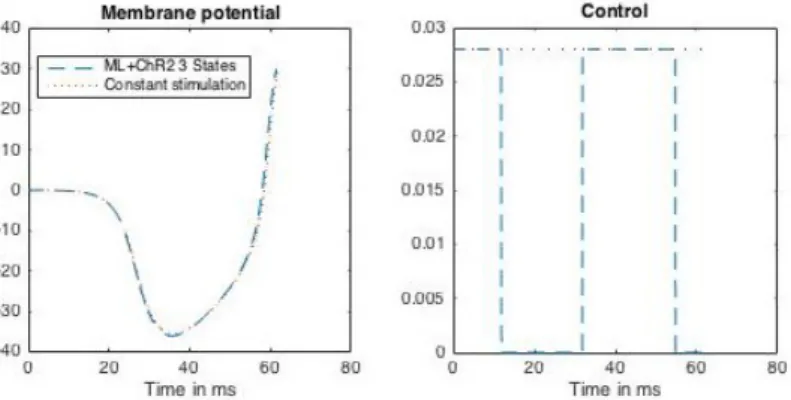
For this model, we implemented the direct method with the numerical values of Appendices A and C.1. The targeted action potential has been fixed to 30mV.
The optimal control for the ChR2-3-states model is bang-bang and begins with a maximal arc. For the numerical values of Appendices A and C.1, it displays three switching times. We represent on Figure 9 the optimal trajectory of the membrane potential and the optimal control, for the phys-iological value of the maximal value control, computed in Appendix C.1, and also the trajectory obtained under constant maximal stimulation, just to observe that the optimal control obtained is indeed better than the constant maximal stimulation. If the difference is very small, of the order of a millisecond, the counter-intuitive stimulation still outperforms the constant maximal stimulation. In order to show that the difference between the counter-intuitive optimal stimulation and the constant maximal stimulation can be huge, we implement the direct method on a system with different numerical values for the constants of the Morris-Lecar model (the Type I neuron of [29, Table 1], see Table 2, in Appendix C.1 ), and values for the ChR2-3-states model remaining unchanged, except for VChR2= 0.1mV. The result is striking, the constant stimulation even fails
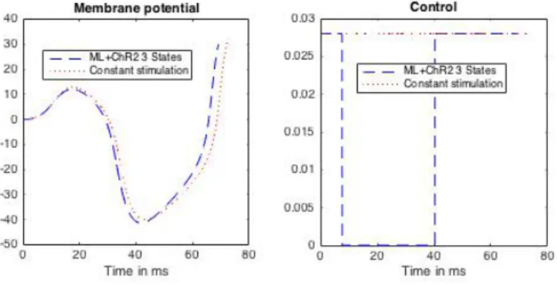
to trigger a spike while the stimulation with three switching times makes the neuron fire (see Figure 10). It is important to note that the presence of three switching times is not an intrinsic characteristic of the Morris-Lecar model itself. Indeed, we can find optimal controls with only two switches if we change the value for the equilibrium potential of the ChR2, keeping all the other constants of the model unchanged (Figure 11).
Figure 10 – Optimal trajectory and bang-bang optimal control for the ML-ChR2-3-states model with numerical values of [29, Table 1]. The constant stimulation fails to trigger a spike.
Figure 11 – Optimal trajectory and bang-bang optimal control for the ML-ChR2-3-states model with numerical values of Appendix A and V ChR2 = 20mV. The optimal control has only two switches.
The ChR2-4-states model
The shape of the optimal trajectory and control of the ChR2-4-states model correspond to the one of the ChR2-3-states model. Nevertheless, for small values of umax, including the physiological
value computed in Appendix C.1, the ChR2-3-states model outperforms the ChR2-4-states model whereas for larger values of umax, the opposite happens (Figure 12). The threshold where this
phenomenon happens is around the value umax = 0.1. Furthermore, the difference grows larger
when umaxincreases. This is an usual behavior that suggests that the Morris-Lecar is less robust
a)
b)
c)
d)
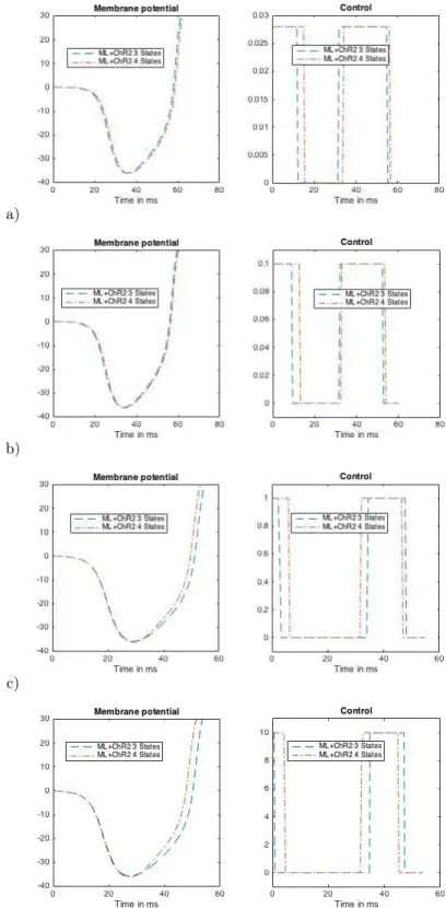
Figure 12 – Optimal trajectory and bang-bang optimal control for the 3-states and ML-ChR2-4-states models with umax=a) 0.028, b) 0.1, c) 1, d) 10 ms 1.
3.3 The reduced Hodgkin-Huxley model
Similarly to the reduction of the initial Morris-Lecar model, there exists a popular reduction of the Hodgkin-Huxley model to a 2-dimensional conductance-based model. This reduction is based on the observation that, on the one hand, the variable m is much faster than the other two gating variables n and h, and on the other hand, the variable h is almost a linear function of the variable n (h ' a + bn). These observations lead to a new system of equations derived from (HH) by setting the variable m in its stationary state m(t) = m1(t)and taking the variable h as above.
(HH2D) 8 > > > > < > > > > : CdV dt = gKn 4(t)(V K V (t)) + gN am31(V )(a + bn(t))(VN a V (t)) + gL(VL V (t)), dn dt = ↵n(V (t))(1 n(t)) n(V (t))n(t), with m1(v) = ↵m(v)
↵m(v) + m(v). It is important to note that, although the time constants of the
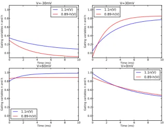
ion channels have been mathematically investigated (see for example [27]), the approximation of the variable h is purely based on observation, and not on a rigorous mathematical reduction. Nevertheless, if the linear approximation seems questionable when the membrane potential is held fixed (Figure 13), it becomes quite remarkable when the whole system (HH) is considered as in Figure 14 for a periodic behavior and Figure 15 for a transitory behavior, with different initial membrane potentials V0. The different behaviors are obtained by tuning the external current Iext
that is applied.
Figure 13 – Linear approximation of the variable h when the membrane potential is held fixed at 30, 0, 30and 60mV.
Figure 14 – Linear approximation of the variable h for a periodic behavior of system (HH) and initial membrane potential of 30, 0, 30 and 60mV.
Figure 15 – Linear approximation of the variable h for a transitory behavior of system (HH) and initial membrane potential of 30, 0, 30 and 60mV.
The ChR2-3-states model
In terms of singular controls, this model behaves similarly to the Morris-Lecar model. There is no singular extremal for the same reasons, and the optimal control is bang-bang with the same expression (the proof is exactly the same). The direct method is implemented with the numerical values of Appendices B and C.1, the targeted action potential has been fixed to 90mV. The optimal control is physiological here and has in fact no switching time, the light has to be on all the way to the spike (see Figure 16).
Figure 16 – Optimal trajectory and bang-bang optimal control for the HH2D-ChR2-3-states model.
The ChR2-4-states model
The ChR2-4-states model is interesting because it shows that the Hodgkin-Huxley behaves in the opposite way of the Morris-Lecar model. Indeed, the ChR2-4-states model slightly outperforms the ChR2-3-states model, and requires less light, for small values of umax, including the physiological
value of umax = 0.028. Furthermore, when umax increases, the 3-states and 4-states models
exactly match, both in terms of optimal trajectory and optimal control (Figure 17). This means that the ChR2-3-states model is a good approximation of the ChR2-4-states model, in terms of optimal control, for the reduced Hodgkin-Huxley. This is a nice property since the ChR2-3-states is theoretically tractable in terms of singular controls.
a)
b)
c)
d)
Figure 17 – Optimal trajectory and bang-bang optimal control for the ChR2-3-states and HH2D-ChR2-4-states models with umax=a) 0.028, b) 0.1, c) 1, d) 10 ms 1.
3.4 The complete Hodgkin-Huxley model
The ChR2-3-states model
The complete Hodgkin-Huxley model is more difficult to analyze mathematically, and optimal singular controls cannot be excluded a priori as for the previous models. Nevertheless, singular controls do not appear in our numerical simulations. Figure 18 shows the optimal trajectory and control for numerical values taken in Appendices B and C.1.
Figure 18 – Optimal trajectory and bang-bang optimal control for the HH-ChR2-3-states model.
The ChR2-4-states model
We observe the same phenomenon than for the reduced Hodgkin-Huxley model, that is, for small values of umax, the ChR2-4-states model slightly outperforms the ChR2-3-states model and when
umax increases, both models match (Figure 19). This constitutes a new argument in favor of
the reduced Hodgkin-Huxley model since it captures the features of the complete model in terms of optimal control. Finally, the fact that both Hodgkin-Huxley models have almost the same behavior for the two ChR2 models means that they can be qualified as robust with regards to the mathematical modeling of ChR2.
a)
b)
c)
d)
Figure 19 – Optimal trajectory and bang-bang optimal control for the 3-states and HH-ChR2-4-states models with umax=a) 0.028, b) 0.1, c) 1, d) 10 ms 1.
3.5 Conclusions on the numerical results
We begin with comments on the two versions of the ChR2 models for each neuron model. For every neuron model that we numerically treat, the ChR2-3-states and the ChR2-4-states versions behave qualitatively the same. We observe no optimal singular controls and the shapes of optimal controls and optimal trajectories are similar. Nevertheless, we can note some distinctions between the neuron models. For the FitzHugh-Nagumo model, the ChR2-4-states version always outperforms the ChR2-3-states version. This is also the case for the two Hodgkin-Huxley models with the important difference that, when the control maximal value increases, the optimal trajectory and optimal control quantitatively match. The Hodgkin-Huxley models are thus very robust with respect to the ChR2 modeling. The Morris-Lecar model displays an unusual behavior when we compare the ChR2-3-states and the ChR2-4-states versions. Indeed, for low values of the control maximal value, including the physiological value computed in Appendix C.1, the ChR2-3-states version outperforms the ChR2-4-states version and the opposite happens when the control maximal value increases.
As announced at the beginning of Section 3, the numerical results invite to distinguish between two main behavior of neuron models with respect to optogenetic control. Most of the models, that is all the models except the Morris-Lecar, behave as physiologically expected. The optimal control is bang-bang, begins with a maximal arc, and has at most one switch. The Morris-Lecar model has more than one switch. This means that it is more efficient to switch on and off the light several times than just keep the light on almost all the way up to the spike. That is why we qualify this model as nonphysiological. Moreover, by only changing the value of the ChR2 equilibrium potential (VChR2) we can observe a change of the number of switches. Finally, the
behavior of the Morris-Lecar model emphasizes the critical importance of optimal control since it allows to find a control that triggers a spike when the expected physiological stimulation (with at most one switch) fails to trigger a spike.
Appendix A Numerical constants for the Morris-Lecar model
The numerical values of the several constants and their physiological meaning are taken from [9] and gathered in Table 1.Table 1 – Meaning and numerical values of the constants appearing in the Morris-Lecar model
V1= 1.2mV Fitting parameter
V2= 18 mV Fitting parameter
V3= 2mV Fitting parameter
V4= 30 mV Fitting parameter
gCa= 4.4 µS/cm2 Maximal conductance of Ca2+channels
gK= 8 µS/cm2 Maximal conductance of K+channels
gL= 2 µS/cm2 Conductance associated with the leakage current
VCa= 120mV Equilibrium potential of Ca2+ions
VK= 84 mV Equilibrium potential of K+ions
VL= 60 mV Equilibrium potential for the leak current
C = 20 µF/cm2 Membrane capacitance
Table 2 gathers the numerical values for Figure 10.
Table 2 – Meaning and numerical values of the constants, taking from [29], appearing in the Morris-Lecar model
V1= 0.01mV Fitting parameter
V2= 0.15mV Fitting parameter
V3= 0.1mV Fitting parameter
V4= 0.145mV Fitting parameter
gCa= 1.0 µS/cm2 Maximal conductance of Ca2+channels
gK= 2.0 µS/cm2 Maximal conductance of K+ channels
gL= 0.5 µS/cm2 Conductance associated with the leakage current
VCa= 1.0mV Equilibrium potential of Ca2+ions
VK= 0.7mV Equilibrium potential of K+ ions
VL= 0.5mV Equilibrium potential for the leak current
C = 1.0 µF/cm2 Membrane capacitance = 0.333 ms 1 Fitting parameter
Appendix B Numerical constants for the Hodgkin-Huxley
model
↵n(V ) = 0.1 0.01V e1 0.1V 1, n(V ) = 0.125e V 80, ↵m(V ) = 2.5 0.1V e2.5 0.1V 1, m(V ) = 4e V 18, ↵h(V ) = 0.07e V 20, h(V ) = 1 e3 0.1V + 1.The following table gathers the numerical values of the Hodgkin-Huxley model, as given in the original paper [16].
Table 3 – Meaning and numerical values of the constants appearing in the Hodgkin-Huxley model
¯
gK= 36 µS/cm2 Maximal conductance of K+channels
¯
gN a = 120 µS/cm2 Maximal conductance of Na2+channels
gL= 0.3 µS/cm2 Conductance associated with the leakage current
EN a= 115mV Equilibrium potential of Na2+ions
EK= 12mV Equilibrium potential of K+ions
EL= 10.6mV Equilibrium potential for the leak current
C = 0.9 µF/cm2 Membrane capacitance
The equilibrium potential ELof the leakage current is usually set so that the equilibrium value of
the (HH) system is such that V = 0.
Appendix C Numerical constants for the ChR2 models
C.1 The 3-states model
The constants of the model are the rates Kd and Kr of the transitions between the open state
and the light adapted closed state and between the two closed states, the maximal conductance gChR2 and the equilibrium potential VChR2. As specified in Section 2, we assume that these rates
are constants during the evolution in order to obtain an affine control system. For the numerical computations, we took the values given in Table 1 of [23]:
Kd= 0.2ms 1, Kr= 0.021ms 1.
The maximal conductance is given by the formula gChR2= ⇢ChR2g⇤ChR2, with ⇢ChR2 the density
of channels and g⇤
ChR2 the conductance of a single channel. These values are taken from [13] to
obtain
gChR2= 0.65mS · cm 2.
As mentioned right after in Appendix B, the physiological equilibrium membrane potential is mathematically shifted to equal 0. The equilibrium potential of the ChR2 that is usually measured around 0 ([13]) and very often taken as 0 ([13],[23]). The exact value 0 would raise a mathematical problem because since we shifted the value of EL so that V = 0 corresponds to the equilibrium
point of the uncontrolled system we start from. Indeed, V = 0 would also correspond to an equilibrium point of the controlled system, regardless of the value of the control. For this reason, we shifted the value of VChR2 and took it equal to 60mV. This value corresponds to the shift of
the membrane resting potential for the Morris-Lecar and Hodgkin-Huxley models.
Finally we can give an estimation of the physiological maximal value umaxof the control. Indeed,
upon illumination, the transition rate between the dark adapted closed state and the open state in [23] is "F where " = 0.5 is the quantum efficiency and F is given by the formula
F = ret wloss
,
where ret ' 10 8µm2 is the retinal cross section (cross section of the photon receptor on the
ChR2), = 6.2 ⇥ 109 ph · µm 2· s 1is the original flux of photons and w
loss= 1.1is a loss factor.
As for the numerical value of Kd and Kr we took the one of Table 1 in [23] for the value of .
With these values we get
umax= 0.028ms 1.
C.2 The 4-states model
The numerical values for the ChR2-4-states model are taken from [13] and gathered in Table 4 below
Table 4 – Numerical values of the constants appearing in the ChR2-4-States model
Kd1= 0.13 ms 1 Decay rate
Kd2= 0.025 ms 1 Decay rate
e12= 0.053 ms 1 Transition rate
e21= 0.023 ms 1 Transition rate
Kr = 0.004 ms 1 Recovery rate
"1 = 0.5 Quantum efficency for o1
"2 = 0.1 Quantum efficency for o2
g1= 50 fS o1state conductance
⇢ = 0.05 Relative conductance of the open states ⇢⇤ChR2= 130 µm 2 ChR2 density
gChR2= 0.65 mS· cm 2 ChR2maximal conductance
References
[1] A.R. Adamantidis, F. Zhang, A.M. Aravanis, K. Deisseroth, and L. de Lecea. Neural sub-strates of awakening probed with optogentic control of hypocretin neurons. Nature, 450:420– 424, 2007.
[2] B. Bonnard and I. Kupka. Théories des singularités de l’application entrée/sortie et optimalité des trajectoires singulières dans le problème du temps minimal. Forum Math., 5:111–159, 1993.
[3] E.S. Boyden. Optogenetics and the future of neuroscience. Nature Neuroscience, 18:1200– 1201, 2015.
[4] E.S. Boyden, F. Zhang, E. Bamberg, G. Nagel, and K. Deisseroth. Millisecond-timescale, genetically targeted optical contro of neural activity. Nature Neuroscience, 8(9):1263–1268, September 2005.
[5] E. Brown, J. Moehlis, and P. Holmes. On the phase reduction and response dynamics of neural oscillator populations. Neural Comput., 16(4):673–715, 2004.
[6] Y. Chen, M. Xiong, and S.C. Zhang. Illuminating Parkinson’s therapy with Optogenetics. Nat. Biotechnol., 33(2):149–150, 2015.
[7] K. Deisseroth. Optogenetics. Nature Methods, 8:26–29, 2011.
[8] K. Deisseroth. Optogenetics: 10 years of microbial opsins in neuroscience. Nature Neuro-science, 18:1213–1225, 2015.
[9] S. Ditlevsen and P. Greenwood. The morris-lecar neuron model embeds a leaky integrate-and-fire model. J. Math. Biol., 67(2):239–259, August 2013.
[10] J. Feng and H.C. Tuckwell. Optimal control of neuronal activity. Phys. Rev. Lett., 91(1), 2003.
[11] R. FitzHugh. Impulses and physiological states in theoretical models of nerve membrane. Biophysical J., 1(6):445–466, 1961.
[12] R. Fourer, D.M. Gay, and B.W. Kernighan. AMPL: A Modeling Language for Mathematical Programming. Duxbury Press, 2002.
[13] T.J. Foutz, R.L. Arlow, and C.C. McIntyre. Theoretical principles underlying optical stimula-tion of a channelrhodopsin-2 positive pyramidal neuron. J. Neurophysiol., 107(12):3235–3245, 2012.
[14] B.M. Gaub, A.E M.H. Berry, Holt, E.Y. Isacoff, and J.G. Flannery. Optogenetics vision restoration using rhodopsin for enhanced sensitivity. Molecular Therapy, 23(10):1562–1571, 2015.
[15] P. Hegemann, S. Ehlenbeck, and D. Gradmann. Multiple photocycles of channelrhodopsin. Biophys. J., 89:3911–3918, 2005.
[16] A.L. Hodgkin and A.F. Huxley. A quantitative description of membrane current and its application to conduction and excitation in nerve. J. Physiol., 117:500–544, 1952.
[17] H. Lecar and C. Morris. Voltage oscillations in the barnacle giant muscle fiber. Biophysical J., 35:193–213, 1981.
[18] M.K. Lobo, E.J. Nestler, and H.E. Covington. Potential utility of Optogenetics in the study of depression. Biol. Psychiatry, 71(12):1068–1074, 2012.
[19] A. Lolov, S. Ditlevsen, and A. Longtin. Stochastic optimal control of single neuron spike trains. J. Neural. Eng., 11, 2014.
[20] A. Nabi and J. Moehlis. Single input optimal control for globally coupled neuron networks. J. Neural Eng., 8:3911–3918, 2011.
[21] J. Nagumo, S. Arimoto, and S. Yoshizawa. An active pulse transmission line simulating nerve axon. Proc IRE, 50(10):2061–2070, 1962.
[22] K. Nikolic, P. Degenaar, and C. Toumazou. Modeling and engineering aspects of channel-rhodopsin2 system for neural photostimulation. Proc. 28th IEEE Eng. Med. Biol. Soc. Conf., pages 1626–1629, 2006.
[23] K. Nikolic, N. Grossman, M.S. Grubb, J. Burrone, C. Toumazou, and P. Degenaar. Photo-cycles of channelrhodopsin-2. Photochemistry and Photobiology, 85:400–411, 2009.
[24] J.T. Paz and J.R. Huguenard. Optogenetics and epilepsy: past, present and future. Epilepsy Curr., 15(1):34–38, 2015.
[25] L. Pontryagin, V. Boltyanski, R. Gamkrelidze, and E. Michtchenko. Théorie mathématique des processus optimaux. Editions Mir, Moscou, 1974.
[26] J. Rinzel. Excitation dynamics: insights from simplified membrane models. Federation Proc., 44:2944–2946, 1985.
[27] J. Rubin and M. Wechselberger. The selection of mixed-mode oscillations in a Hodgkin-Huxley model with multiple timescales. Chaos, 18(1):015105, 2008.
[28] T.J. Ryan, D.S. Roy, M. Pignatelli, A. Arons, and S. Tonegawa. Engram cells retain memory under retrograde amnesia. Science, 348(6238):1007–1013, 2015.
[29] M. Saint-Hilaire and A. Longtin. Comparison of coding capabilities of type I and type II neurons. Journal of computational neurosciences, 16:299–313, 2004.
[30] E. Trélat. Contrôle optimal : théorie et applications. Vuibert, 2008.
[31] E. Trélat. Optimal control and applications to aerospace: some results and challenges. J. Optim. Theory Appl., 154(3):713–758, 2012.
[32] J. Wong, O.J. Abilez, and E. Kuhl. Computational optogenetics: a novel continuum frame-work for the photoelectrochemistry of living systems. J. Mech. Phys. Solids., 60(6):1158–1178, 2012.
[33] A. Wächter and L.T. Biegler. On the implementation of an interior-point filer line-search algorithm for large-scale nonlinear programming. Math. Program., 106:25–27, 2006.