Characterizing the dam break release

Characterizing the Dam Break Release

by

Juliana Wu

Submitted to the Department of Mechanical Engineering

in partial fulfillment of the requirements for the degree of

Bachelor of Science in Mechanical Engineering

at the

MASSACHUSETTS INSTITUTE OF TECHNOLOGY

June 2014

Massachusetts Institute of Technology 2014. All rights reserved.

A uthor ...

Certified by...

Signature redacted

Department of Mechanical Engineering

May 9th, 2014

Signature redacted

Alexandra Techet

Associate Professor

Thesis Supervisor

Signature redacted

Accepted

by...

...

Anette Hosoi

Professor of Mechanical Engineering

Undergraduate Officer

MASSACHUSETFS INS"I'll Ui E OF TECHNOLOGY

JUL 3

0

2014

Characterizing the Dam Break Release

by

Juliana Wu

Submitted to the Department of Mechanical Engineering on May 9th, 2014, in partial fulfillment of the

requirements for the degree of

Bachelor of Science in Mechanical Engineering

Abstract

The failure of a dam can cause disastrous consequences, thus understanding the nature of a dam break is of utmost importance. A model of a dam break was built and used to profile the resulting wave. The gate release was characterized to check for consistency, maximum velocity, and it's profile. Matlab code was created to analyze both the gate speed and the wave velocity. The maximum velocity was 1503.2 cm/s and there a

30% deviation at most.The wave velocity was found to increase as the water reservoir

height was increased. An equation was derived that had a 0.96 correlation coefficient thus proving that the relationship between velocity and reservoir height was accurate. Further research can be done using a cantilevered plate downstream of the dam break to analyze the forces generated.

Thesis Supervisor: Alexandra Techet Title: Associate Professor

Acknowledgments

I would like to thank Professor Techet for giving me the opportunity to UROP for

the past couple years in her lab. It has been a great experience learning how to do many things from underwater 80/20 to image processing in Matlab. Thank you so much.

I would also like to thank Leah Mendelson who has advised me and helped me with so much. Thank you for taking your time to be my mentor for the past couple years. From teaching me how to use the high speed camera array to take videos of fish to how to properly cite in LaTeX, you have taught me so much and I can't even explain how grateful I am.

Thanks to Barry Scharfman and Abhishek Bajpayee for answering all my questions on Matlab, image processing, and how I should be analyzing my data. My thesis would not be complete without you.

Thank you to Emma Nelson for coming in on Friday mornings and weekends to help me take data. Without you I would not have survived this semester. Your cheerfulness and great attitude always lightened my day.

Thanks to Alex Willisson for helping me keep my sanity and for keeping me on track with reality.

Lastly, thank you to Jaymond Chan for all the emotional support throughout this process. I would not have been able to finish my thesis without you.

Contents

1 Introduction

2 Experimental Set Up 2.1 Dam Break Model

2.2 Pneumatic System

2.3 Cameras and Lights.

3 Characterizing the Gate

3.1 Setup . . . .

3.2 Analysis . . . .

3.3 Results . . . .

Release

4 Characterizing the Dam Break Release

4.1 Setup. ... 4.2 Analysis ... ... 4.3 Results ... 5 Conclusion A Tables B Figures 13 15 15 15 16 19 19 19 20 23 23 23 25 29 31 33 . . . . . . . . . . . . . . . . . . . . . . . .

List of Figures

2-1 Diagram of Experimental Setup . . . .

3-1 Examples of Gate Release Graphs . . .

Analysis Image Progression . . . .

Example Images of Wave Profile . . . . . Smoothed plots . . . .

Example of Wave Profile Analysis . . . .

Example of Original Gate Speed Image Example of Gate Speed Analysis Images Data for Gate Speed Analysis . . . .

Data for Wave Velocity Profile(1) . . . .

Data for Wave Velocity Profile(2) . . . .

Data for Wave Velocity Profile- Incorrect Data for Wave Velocity Profile- Incorrect

24 25 26 27 Calibration (52 cm) Calibration (38 cm) . . . . 33 . . . . 34 . . . . 35 . . . . 36 . . . . 37 . . . . 38 . . . . 39 16 . . . . 20 4-1 4-2 4-3 4-4 B-1 B-2 B-3 B-4 B-5 B-6 B-7

List of Tables

3.1 Maximum Gate Speed ... 21

Chapter 1

Introduction

Dams are structures that primarily retain large amounts of water for either collection or storage for future distribution. Often hydropower and pumped-storage hydro-electricity are implemented with dams to generate hydro-electricity. However disastrous consequences happen when a dam fails and the structure is breached or damaged. In

1975, 171,000 people were killed and 11 million people were left homeless in the failure

of the Banqiao Reservoir Dam in the Henan Province of China. If the designers of the dam had taken into account how the dam break water would flow, then those people and their homes may have been saved from disaster. Research into dam break water flows also applies to problems caused by rouge waves hitting structures such as a ship hull. Rouge waves have had a history of causing immense damage to unsuspecting structures; but by understanding the nature of the dam break, engineers will be able to prevent some of resulting damage.

The 19th century contains the first studies analyzing dam break flows. The free-surface profile evolution for a collapsing rectangular column of fluid over a dry hor-izontal downstream bed was published by Ritter in 1892 [2]. Ritter published a theoretical solution based on the shallow water theory, but neglected both turbulence effects and friction over the bed. There have been numerous experimental studies on dam break flow, however not much research have studied the dynamics of the flow.

The Maritime Research Institute of the Netherlands used an experimental work to validate their numerical scheme describing the dam break wave kinematics [3]. They

also collected data of a wave impact downstream of the dam break on a solid vertical wall. They used force transducers with large circular impact panels to measure the impact pressure at different locations.

Their experimental setup was used in further experiments such as the recent in-vestigation by Lobovskf et al [1]. Lobovskf et al. conducted numerous experimental measurements on a dam break flow over a horizontal dry bed to give further insight on the dynamics of a dam break wave impact on a vertical wall. They also analyzed the kinematics of the free surface and wave front evolution. Furthermore, his work

and observations agree with existing literature.

This thesis aims to analyze the wave speed velocity upon release from a dam break. Furthermore, this work intends on confirming the consistency of the gate speed upon release. The results from this research will serve as the foundation for future experiments with the same dam break experimental set up.

Chapter 2

Experimental Set Up

2.1

Dam Break Model

A model of a dam break was designed and built in order to characterize the release. A large glass tank with length of 327.6 cm, width of 91.4 cm, height of 81.2 cm, and a

thickness of 1.9 cm was used to hold a metal reservoir of water. False walls, back, and bottom were installed in the glass tank in order to prevent the release of the water from harming the tank and to normalize the release. There was a distance of 63.75 cm between the false walls and a distance of 92.1 cm between the false back and the edge of the false wall. The false walls ran from the edge of the metal reservoir for

132.5 cm. The metal reservoir itself was a rectangular prism with a length of 86.5 cm, width of 71.4 cm and a height of 121.9 cm. On the release face of the reservoir,

a gate was added with a pneumatic system.

2.2

Pneumatic System

The pneumatic system pressurizes a cylinder with two compartments separated by a piston which is connected to the release gate. The compartments of the cylinder are connected to a switch valve. The switch valve has one input and two outputs, one to the top compartment of the cylinder and one to the bottom compartment of the cylinder. An air gun is connected to the input to pressurize the system. The switch

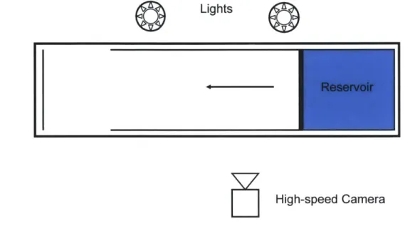
Figure 2-1: This is a top view diagram of the experimental set up. The camera was placed in front of the tank while the two strobe lights were behind with the timing box. The metal reservoir holding the water was in the glass tank between the false walls.

6;jN Lights 6

High-speed Camera

controls the airflow from one compartment to the other compartment. When the gate is released, air flows from the top compartment and into the bottom compartment so that the pressure in the bottom compartment is greater than in the top. When the gate is closed, air flows from the bottom compartment and into the top compartment so that the top compartment pressure is greater than the bottom.

2.3

Cameras and Lights

Two strobe light banks were placed behind the glass tank to ensure even light and were timed using a multi-trigger digital delay generator. White paper was placed between the glass tank and the light banks to make a clean background. A Phantom Miro High Speed Camera was placed in front of the glass tank to capture the release of the wave. The high speed camera was connected using an Ethernet cable to a laptop which used the Phantom Camera Control software to record the release at

16

high speeds. A 50 mm Nikon camera lens was used with a focal length of either 11 or 8.6 depending on the data taken.

Chapter 3

Characterizing the Gate Release

3.1

Setup

In order to characterize the dam break, the gate release had to be defined. Three white squares were attached to the gate at 15 cm intervals. A mirror was set up at a 45 degree angle so that the camera would have a front view of the gate and the squares. When the gate was released, the camera recorded the squares as they traveled through the field of view. Calibration was taken before and after the test runs each day. To calibrate, a grid of 2.065 cm black and white squares was placed on the gate and was used to determine a pixel to length scale.

3.2

Analysis

Matlab code was created to analyze the data. The gate speed code began by setting up an array with the images that were to be analyzed. The code then changed each image to a black and white image and found the centroids for any squares that were in the images. A separate array containing all the data was created and maintained throughout scanning every image. After all the images were analyzed, the code implemented a tracking function which tracks particles as they move throughout space and time. For the purpose of this thesis, the three squares were tracked and their distance through time was plotted on a graph. After their distances were plotted,

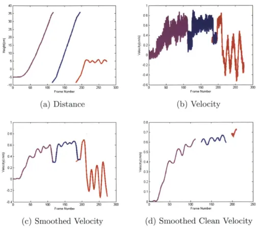
Figure 3-1: In (a) the height of each square was measured as they traveled through time. (b) shows the velocity of the squares calculated from the distances. The velocity was smoothed using a smoothing function in Matlab in (c). Finally in (d) the areas where the squares entered and left the field of view were removed.

35 30 25 20 15 10 -5 o0 o s lEA 2M8 25) 31 Frame Number (a) Distance 08 0.6 0.4 02 0 -0.2 -0.4 0 oj 15) 150 2W2 2M) Frame Number (c) Smoothed Velocity 10 06 0.4-(b) Velocity 0-0.7 06 05 03 0.2 01 0 5)) 100 150W 8 2-5 Frame Number

(d) Smoothed Clean Velocity

a preliminary velocity graph was generated. Because of the large amount of noise due to recording at 2000 frames per second, a secondary smoothed velocity graph was generated. Finally, the places on the graph where the squares were entering and leaving the field of view were removed because the centroids gave incorrect tracking data thus causing incorrect fluctuations.

3.3

Results

The gate speed was analyzed at three different water reservoir heights. Data was taken twice at 20 cm, 25 cm, and 30 cm. For all six runs, the pneumatic system was pressurized to 150 Psi and the air compressor would automatically turn off signally that the gate was ready to be released. The gate had to be released within 1 minute

20

,vvA q/

U

or else the pneumatic system would lose too much pressurized air and then the gate release would not be at 150 Psi. All six runs showed a general trend in the smoothed velocity plots. The velocity curve begins at 0 cm/s, then as the gate is released there is a sharp acceleration. After a certain point, the acceleration decreases and the velocity increases until the gate is fully opened. At this point the gate begins vibrating causing rapid fluctuations which were removed from the graph.It can be deduced that as the gate open and water rushed out, there would be less resistance against the gate which would allow it to accelerate faster. However at one point, the pressurized air would escape and the acceleration would slow down.

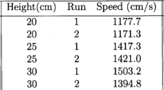
From the velocity graphs, the max velocity that the gate reached was recorded in Table 3.1. The maximum of all the gate speeds reached 1503.2 cm/s. The difference between the two extreme maximums was 331.9 cm/s. This large difference may be due to the 2000 frames per second frame rate which caused large amounts of noise in the data. Furthermore, all the gate speed maximums were within 30% of each other.

Table 3.1: Maximum Gate Speed

Height(cm) Run Speed (cm/s)

20 1 1177.7 20 2 1171.3 25 1 1417.3 25 2 1421.0 30 1 1503.2 30 2 1394.8

Chapter 4

Characterizing the Dam Break

Release

4.1

Setup

After the gate release was characterized, the dam break wave profile was then studied. The high speed camera was set up near the gate release so that the field of view captured the wave profile as it exited the reservoir. Calibration was taken before and after the test runs each day. A grid of 2.065 black and white squares was placed in the middle of the tank so that the camera would focus between the front and back glass wall. Between each run, a pump was used to move water from the glass tank to the reservoir. To change water levels, a secondary pump added or removed water between a sink and the glass tank.

4.2

Analysis

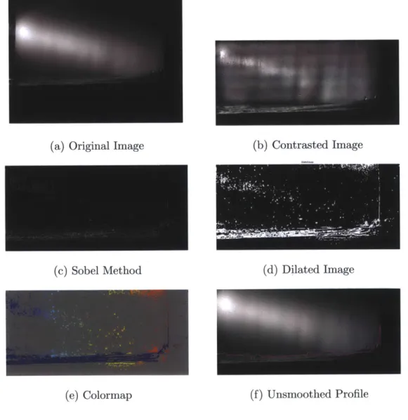
Matlab was again used to analyze the wave profile. The code set up a 3D array where each image was a separate page and tracked all the images through time. Each image was changed to black and white and then cropped so only the pertinent area was stored. The image contrast was then enhanced and a "wiener2" lowpass filter removed some noise. Afterwards the code tracked the edge of the image using

the Sobel method and dilated the black and white edges with discs. Next the code looked for areas where the discs overlapped and connected the area where the disks overlapped the most to form the wave profile. To analyze the wave velocity, the front

Figure 4-1: The original image is shown in (a) while the Wiener2 filter was applied in the contrast image in (b). (c) shows the edge detection using the Sobel method which was then dilated in (d). The areas which were connected was shown in a colormap in

(e) and the unsmoothed profile was then calculated and plotted in (f).

(a) Original Image (b) Contrasted Image

(c) Sobel Method (d) Dilated Image

(e) Colormap (f) Unsmoothed Profile

edge of the wave was tracked as it progressed through time and then plotted. A line was fitted to the data and the resulting slope was the velocity of the wave profile.

4.3

Results

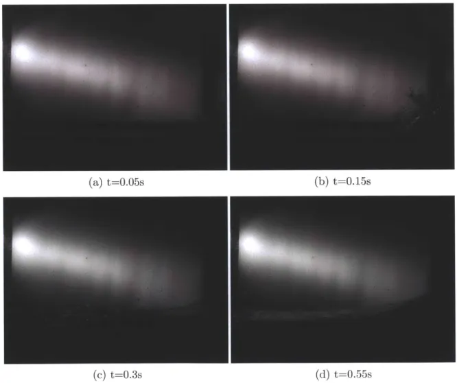
An example of the resulting smoothed curve is shown in Figure 4-2. All wave profiles followed the same general trend. As the gate was released, there was a violent and turbulent spray of water as it escaped through the bottom of the gate. The wave forms ligaments and droplets as it continues to rush out of the gate.

Figure 4-2: The wave profile is shown in these images. In (a) the gate has just begun moving and water is beginning to leave the reservoir. (b) shows the turbulence as the water violently rushes out. (c) shows the smooth wave profile beginning to form while the wave front is still turbulent. In (d) the wave profile is smooth and has settled.

(a) t=0.05s (b) t=0.15s

(c) t=0.3s (d) t=0.55s

As the wave continues through the tank, it calms down to a more smooth curve with the front of the wave still turbulent. After the front of the wave passes out of the camera's field of the view, the rest of the wave is a smooth curve. The two sides

of the wave are higher than the center due to capillary action along the tank's false walls. The edge of the wave along the back false wall was also out of focus compared to the area closer to the front false wall.

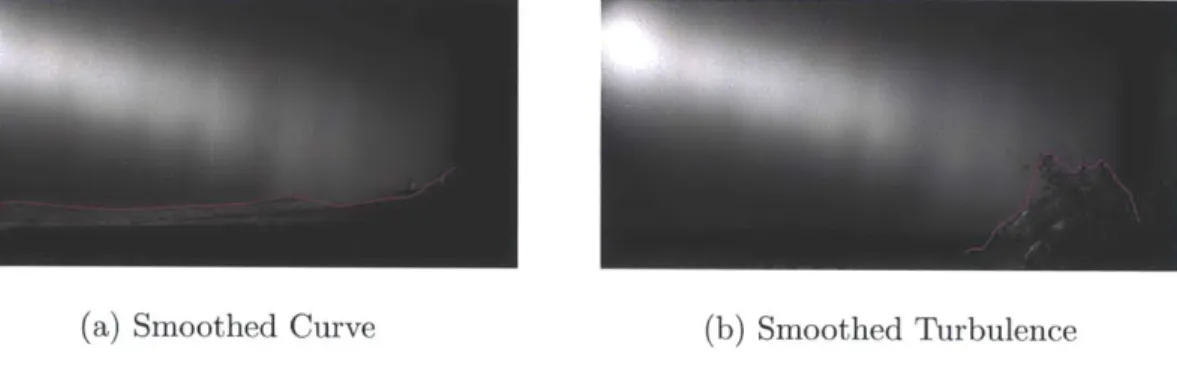
Figure 4-3: In (a), the smoothed curve is plotted for a relatively smooth wave profile. There are areas where the curve does not perfectly trace the wave profile, however the majority of the back wave profile is traced. In (b), the turbulence makes it hard for the code to distinguish where exactly is the water. The code does manage to trace the majority of the droplets that form from the turbulence.

(a) Smoothed Curve (b) Smoothed Turbulence

A smoothed curve was then plotted using the methods discussed in the previous

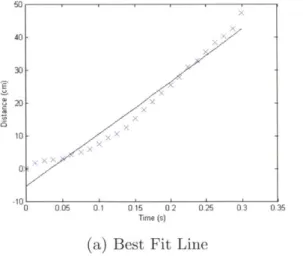
analysis section. There were some areas of the wave which were not included in the curve due to the lightning on the water. The Matlab code could not differentiate between the background light that part of the water profile. Furthermore the turbu-lent wave front causes the curve to be rough as the code believes all the droplets and ligaments as part of the wave profile itself. The wave velocity was calculated for three different water heights: 15 cm, 25 cm, and 40 cm. The 25 cm and 40 cm were run twice while the 15 cm was only run once. An example of the resulting distance plot and best fit line is shown in Figure 4-4. The average velocities were found and are shown in Table A-1. The higher water height in the reservoir had faster wave velocity as the gate was released. There were more runs taken, however the calibration for those runs were incorrect thus resulting in an inaccurate measure of the wave velocity. The resulting graphs and spline measurements are found in the Appendix. A second order spline was also fitted to each of the velocity curve and can also be found in the Appendix.

The following equation was derived to describe the relationship between the

Figure 4-4: In (a), a best fit line is plotted against the distance of the wave front data. In (b), a second order spline is fitted to the distance data.

50 40 30 ~20 10 0:

-

(a) Best Fit Line

50 30 ~20 10 G: 0.35 0 0.05 0.1 0.15 02 0.25 Time (s)

(b) Second Order Spline

voir water height and the resulting wave velocity.

Velocity = 3.304 x Water Height + 102.04 (4.1)

The line had a 0.96 correlation coefficient thus is an acceptable descriptor of the relationship between water height and velocity.

-7

-7

0.3 0.35

lu

Chapter 5

Conclusion

Because a dam failure can cause disastrous consequences, it is necessary to understand the nature of a dam break. A model dam break scenario was designed and constructed to learn more about the characteristics behind a dam break. First the gate speed release was found reach a maximum velocity of 1503.2 cm/s. There was a 30% difference between the lowest maximum velocity and the highest maximum velocity. However, this difference can possibly due to the large number of frames per second which added noise to the data. Second, the dam break wave velocity was calculated for several water reservoir heights. As the water height was increased, the resulting wave velocity also increased. An equation was derived which had a .96 correlation coefficient thus being an accurate descriptor of the relationship.

Future work can be continued with this project such as finding an accurate equa-tion for the wave curve as it exits the reservoir. Also, the maximum height the wave reaches for every water reservoir height would be another extension to this project. More repetitions with proper calibration would also be useful to check for consistency. To understand more about rouge waves, a cantilevered plate could be installed down-stream of the dam break and the resulting forces can be measured. The results of this research can be applied to real world situations where people can be alerted as to how fast a dam failure wave will reach their location.

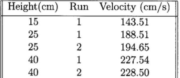
Table A. 1: Maximum Wave Velocity

Height(cm) Run Velocity (cm/s)

15 1 143.51 25 1 188.51 25 2 194.65 40 1 227.54 40 2 228.50

Appendix A

Tables

Appendix B

Figures

Figure B-2: Example of Gate Speed Analysis Images

(a) Black and White Cropped (b) Centroids Located

Figure B-3: Data for Gate Speed Analysis 0.51 0.4 0.3 0.2 0.1 0 -0.1 0.7 0.6 0.5 04 03 02 01 0 0 10 16 0 so 100 150 Frame Number (a) 20 cm Run 1 0 20 40 60 80 100 120 140 160 180 20 Frame Number (c) 25 cm Run 1 0.8 0.7 06 0.5 0.4 0.3 0.2 0.1 0 -0.1 0 20 40 60 80 100 120 140 160 180 20 Frame Number (e) 30 cm Run 1 6 06 05 0.4 0.3 0.2 01 0 -0 1 0 0B 0.7 06 0.5 04 > 0.3 02 0.1 a 0 0.7 0.6 0.5 0.4 > 0.3 0.2 0.1 0 U a 50 100 150 2) 2-Frame Number (b) 20 cm Run 2 U 20 40 60 80 100 120 140 160 180 2C Frame Number (d) 25 cm Run 2 80 10-6 50 100 150 Frame Number (f) 30 cm Run 2 200 00

Figure B-4: Data for Wave Velocity Profile(1) 80 70 60 ~50 40 30 20 10 0 0.05 0.1 0.15 0.2 025 0.3 0.35 0.4 0.45 Time (s) u 70 60 50 40 30 20 10 -, -, 00 0.05 0.1 0,15 0.2 0.25 0.3 0.35 0.4 0.45 0.5 Time (s) (b) 15 cm: y=44.085x2+ 133.54x + 3.58 0.5 (a) 15 cm: y=43.51x-3.87 80 707 60 50 40 30 20 10 x' 0 0 0.05 0.1 0.15 0.2 0.25 0.3 035 0. Time (S) 70 60 50 40 ~30 20 10 (c) 25 cm Run 1: y=188.51x-1.05 60 50 -40 30 20 Kx 10 x 0 0 0. 0.'1 0.15 0,2 0. 0.3 0,35 Time (s)

(e) 25 cm Run 1: y=194.65x+0.72

x -0 .6 01 01x. .6 03 03 .

0

Figure B-5: Data for Wave Velocity Profile(2) 50 x 40 X. 30 20 102 -10 0 0.0 0.1 0,15 0.2 0.25 0,3 0-, Time (s)

(a) 40 cm Run 1: y=227.54x-6.59

40 35 30 ~26 20 i5 15 10 0 0 0.05 0.1 0.15 0.2 Time (s) 025 50 40 30 ~20 10 0 005 01 0.15 02 Time (s) 025 03 0 (b) Run 1: y=378.51x2 _{+ 95.08x} '5 0 3 035 (c) 40cm Run 2: y=228.5x-9.01 45 40 35 30 25 20 15-10. 5 0 0.05 0.1 0.15 0.2 Time (s) 0.18 025 0.3 0,35 -7 --x,. (d) Run 2: y=383.76x2_{+ 95.59x - 0.89} -W

Figure B-6: Data for Wave Velocity Profile- Incorrect Calibration (52 cm) 40 3U 20 x x 0 S 0.05 0.1 0.15 0 2 025 0.3 0,35 Time (s)

(a) Run 1: y=159.04x-5.3517

40 35 30 25 20 i 15-10 5 x 4/ 0 005 0.1 0.15 02 0.25 0.3 0 0,05 O.A 0.16 0,2 0.25 0.3 Time (s) (c) Run 2: y=160.0x-4.35 6 40 30 20 10 0 0.05 01 0.15 0.2 025 Time (s) 03 0.35 (b) Run 1: y=365.44x2 _{+ 49.41x - 0.09} 45 40 35 30 25 20 15 -10 035 0 0.05 0.1 0.15 0.2 0.25 0.3 Time (s) 0.35 (d) Run 2: y=285.08x 2+ 82.26x - 0.09 38

Figure B-7: Data for Wave Velocity Profile- Incorrect Calibration (38 cm) 0 0.05 0.1 0.15 0.2 0.25 0.3 Time (s) 70 60 50 40 30 20 10 0: 0.35 0 0.05 0.1 0.15 0.2 Time (s) 025 03 0.35

(a) Run 1: y=158.22x-3.87

0.05 0.1 0 15 0,2 0.25 Time (s) 0.3 0.35 0.4 (c) Run 2: y=156.lx-1.05 (b) Run 1: y=309.67x2 + 69.19x + 0.21 90 70 60 0 0.05 0.1 0.15 0.2 Time (s) 0.25 0.3 0,35 0.4 (d) Run 2: y=196.17x 2 + 104.6x + 1.097 60 50 40 30 20 10 0 K 4 K ;2 0 70 60-50 40 !30 20 10 0" -10 0

xx

Bibliography

[1] Libor Lobovsky, Elkin Botia-Vera, Filippo Castellana, Jordi Mas-Soler, and

An-tonio Souto-Iglesias. Experimental investigation of dynamic pressure loads during dam break. arXiv preprint arXiv:1308.0115, 2013.

[2] August Ritter. Die fortpflanzung de wasserwellen. Zeitschrift Verein Deutscher

Ingenieure, 36(33):947-954, 1892.

[3] ZQ Zhou, JO De Kat, and B Buchner. A nonlinear 3d approach to simulate green

water dynamics on deck, presented at 7th int. In Conference on Numerical Ship