Chasing ancient demons : tools for measuring 21 cm fluctuations before reionization

(1)

Chasing Ancient Demons:

cm Fluctuations before Reionization

by

Aaron Ewall-Wice

B.A., University of Chicago (2011)

Submitted to the Department of Physics

in partial fulfillment of the requirements for the degree of

Doctor of Philosophy

at the

MASSACHUSETTS INSTITUTE OF TECHNOLOGY

MAss S INSTITUTE OF T CrHN0LOGY

JUN 2 77017

LIBRARIES

June 2017

@

Massachusetts Institute of Technology 2017. All rights reserved.

Author

Signature redacted

Department of Physics

May 23rd, 2017

Certified by..

Accepted by

Signature redacted

Jacqueline Hewitt Professor of Physics Thesis Supervisor

..

Signature redacted...

Nergis Mavalvala

Professor of Physics

Associate Department Head for Education

(2)

77 Massachusetts Avenue Cambridge, MA 02139 http://Iibraries.mit.edu/ask

MITLibraries

DISCLAIMER NOTICE

Due to the condition of the original material, there are unavoidable flaws in this reproduction. We have made every effort possible to provide you with the best copy available.

Thank you.

*Some pages in the original document contain text that runs off the edge of the page.

(See pages 203 & 303)

(3)

(4)

Chasing Ancient Demons: Tools for measuring 21 cm

Fluctuations before Reionization

by

Aaron Ewall-Wice

Submitted to the Department of Physics on May 23rd, 2017, in partial fulfillment of the

requirements for the degree of Doctor of Philosophy

Abstract

In this thesis, we take the first steps towards measuring the fluctuations in HI emission before reionization which carry information on the first X-ray emitting compact ob-jects and hot interstellar gas heated by the deaths of the first stars (ancient demons). First, we show that existing and planned interferometers are sensitive enough to place interesting constraints on the astrophysics of X-ray heating. Second, we obtain first upper limits on the pre-reionization fluctuations with the Murchison Widefield Array. We also use these measurements to explore the impact of low-frequency systematics, such as increased foreground brightness and the ionosphere.

We discover that contamination by fine-scale frequency structure introduced by the instrument is the leading obstacle to measuring the 21 cm power spectrum before reionization. This motivates the design of a next-generation experiment, HERA, with acceptable levels of intrinsic spectral structure. We also perform a careful examination of whether traditional calibration strategies are sufficient to suppress instrumental spectral structure. We find that while existing calibration techniques have critical flaws, there exist promising strategies to overcome these deficiencies which we are now pursuing.

Thesis Supervisor: Jacqueline Hewitt Title: Professor of Physics

(5)

I became aware of the old island here that flowered once for Dutch sailors' eyes - a fresh, green breast of the new world. Its vanished trees, the trees that had made way for Gatsby's house, had once pandered in whispers to the last and greatest of all human dreams; for a transitory enchanted moment man must have held his breath in

the presence of this continent, compelled into an aesthetic contemplation he neither understood nor desired, face to face for the last time in history with something

commensurate to his capacity for wonder. F. SCOTT FITZGERALD

(6)

4.6.3 How well do Epoch of X-ray Heating measurements improve Constraints on Reionization? . . . . 4.6.4 Overall Parameter Constraints . . . . 4.7 Conclusions . . . . 5 First Limits on the 21 cm EoX Power Spectrum 5.1 Introduction . . . . 5.2 Observing and Initial Data Reduction . . . . 5.2.1 Observations with the MWA . . . . 5.2.2 RFI flagging and Initial Calibration . . . . 5.2.3 MFS Imaging and Flux Scale Corrections . . . . 5.2.4 Data Cubes for Power Spectrum Analysis . . . 5.3 Addressing the Challenges of Low Frequency Observing 5.3.1 Radio-Frequency Interference . . . . 5.3.2 Ionospheric Contamination . . . . 5.3.3 Instrumental Spectral Structure . . . . 5.3.4 Calibration with Autocorrelations . . . . 5.3.5 The time dependence of residual structure. . . . 5.4 Power Spectrum Results . . . . 5.4.1 Systematics in the 2d Power Spectrum. . . . . . 5.4.2 Comparing Calibration Techniques . . . . 5.4.3 Power Spectra Comparison Between Nights of spheric Activity . . . . . . . . 198 . . . . 199 . . . . 200 205 . . . . 206 . . . . 210 . . . . 210 . . . . 211 . . . . 216 . . . 218 . . . . 223 . . . 224 . . . . 226 . . . . 234 . . . . 241 . . . . 245 . . . . 247 . . . . 248 . . . . 253 Varying Iono-257

(10)

5.4.4 First Upper Limits on the 21 cm Power Spectrum During the

Pre-Reionization Epoch . . . 258

5.4.5 The outlook for EoR Measurements on the MWA. . . . 260

5.5 Conclusions and Future Experimental Considerations . . . 262

5.A Appendix: The Effect of Cable Reflections on Tile Gains . . . 265

5.B Appendix: The Power Spectrum of ionospheric phase fluctuations from measurements of Differential Refraction. . . . 267

5.C Appendix: The Amplitude of Scintillation Noise in MWA Visibilities. 268 6 he HERA Dish II: Electromagnetic Simulations and Science Im-plications 271 6.1 Introduction . . . . ... . . . . 272

6.2 The Impact of Reflections on Delay-Transform Power Spectra . . . . 276

6.3 Electromagnetic Simulations of the HERA dish element . . . 280

6.3.1 The Simulations . . . 281

6.3.2 Deconvolving the Response Function . . . 283

6.4 Simulation Results . . . . 284

6.4.1 The Time Domain Response of the HERA Dish . . . 285

6.4.2 The Delay Response of Subbands . . . 285

6.4.3 The Origin of the Knee. . . . . 287

6.4.4 Tradeoffs in Beam Properties. . . . 290

6.4.5 Verifying Our Framework with S11 Measurements and Simulations293 6.5 The Effect of the Spectral Structure due to Reflections and Resonances in the HERA dish on Foreground Leakage and Sensitivity . . . 296

6.5.1 Extrapolating the Bandpass and Power Kernel . . . 296

6.5.2 The Impact of delay response of the HERA Antenna on Fore-ground Contamination . . . . 298

6.5.3 The Implications of Reflections and Resonances on EoR Science 302 6.6 Conclusions . . . . 310

(11)

7.1 Introduction . . . . 313

7.2 Form alism . . . . 318

7.2.1 The Statistics of Unmodeled Source Visibilities . . . . 319

7.2.1.1 Unmodeled Point Sources . . . 319

7.2.1.2 Diffuse Galactic Emission . . . 320

7.2.2 Frequency Domain Calibration Errors . . . 321

7.2.3 The Impact of Gain Errors on the 21 cm Power Spectrum . . . 325

7.2.4 Calibration Bias for a Simplified Model . . . 330

7.3 Modeling Noise in Existing Arrays . . . 333

7.3.1 Instrumental Models . . . 333

7.3.2 Modeling Results . . . 335

7.3.3 The Impact of Primary Beam Modeling Errors . . . 338

7.3.4 The Dependence of Modeling Noise on Array and Catalog Prop-erties . . . 341

7.3.4.1 Catalog Depth . . . 341

7.3.4.2 Time Averaging . . . 342

7.3.4.3 Array Configuration . . . 343

7.4 Eliminating Modeling Noise with Baseline Weighting . . . 345

7.4.1 Gaussian Weighting for Sky-Based Calibration . . . 347

7.4.2 The Impact of Inverse Baseline Weighting on Power Spectrum Sensitivity . . . 349

7.5 Conclusions . . . 355

7.A Appendix: The Impact of Redundancy . . . 357

7.B Appendix: The Point Source Approximation For Modeled Foregrounds. 360 7.C Appendix: Expressions for Second Moments of Delay-Transformed Calibration Errors. . . . 363

7.C.1 Derivation of Equation 7.29 . . . . 365

7.C.2 Derivation of Equation 7.30 . . . 366

7.C.3 Derivation of Equation 7.31 . . . 366

(12)

7.C.5 Derivation of Equation 7.33 . . . . 367 7.D Appendix: Components of A and IV for Non-Redundant, Uniformly

Weighted Calibration Solutions . . . . 367

7.D.1 Equation 7.36 . . . . 367 7.D.2 Equation 7.37 . . . . 369 7.E Appendix: A Simplified Expression for Minimal Accessible

Line-of-Sight M odes. . . . . 370

8 Conclusion 373

(13)

List of Figures

1-1 The history of our Universe as revealed by cosmological observations.

To date, our direct observations are limited to the "modern universe" (roughly 1 billion years after the big bang) and a thin slice of the early Universe (the CMB). The critical chapters in structure formation, in which the first baryonic objects collapsed and the first stars ignited (the "Dark Ages" and the "Cosmic Dawn") remains mostly beyond the

reach of today's instrumentation. . . . . 52

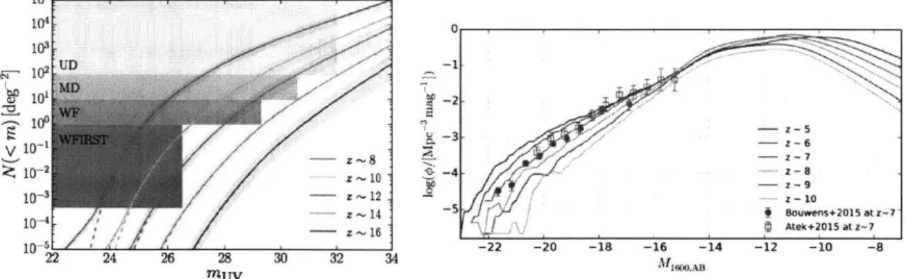
1-2 Left: The number density and apparent IR magnitudes at galaxies during and before reionization along with the coverage of planned sur-veys by JWST and WFIRST from (Mason et al., 2015). Without the assistance of strong gravitational lensing, it will be difficult for IR sur-veys to look beyond reionization. Right: The UV luminosity function predicted by the DRAGONS simulations at several different redshifts

for (Liu et al., 2016). The turnover at MAB = -12 corresponds to

the luminosity of atomic cooling halos and is significantly below the

(14)

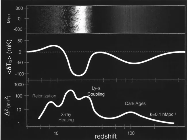
1-3 Top: A two-dimensional slice of the brightness temperature field from

the Evolution of 21 cm Structure (EoS) 2016 data release (Mesinger et al., 2016). Middle: the corresponding global signal being targeted

by single dipole experiments. Bottom: The power spectrum of

bright-ness temperature fluctuations at the k = 0.1 hMpc- 1 scale. The global

signal exibits a z ~ 100 dip which occurs when the rate of collisions

between CMB photons and HI atoms drops due to the Universe's ex-pansion and rises again as collisional coupling to the HI kinetic temper-ature becomes similarly inefficient. Ly-a photons from the first stars

introduce a dramatic falloff at z ~ 30, strongly coupling T, to Tk.

Ts = Tk rises dramatically between 10

3

z

3

20 as X-rays heat the

IGM. As this heating proceeds, high-contrast exists between hot and cold IGM patches introduces significant fluctuations and a maximum

in the power spectrum at z ~ 15. Fluctuations from the ionization field

take over at z

3

10 before reionization eliminates the neutral hydrogen

in the IGM, bringing both the power spectrum and the global signal

to~0... ... 75

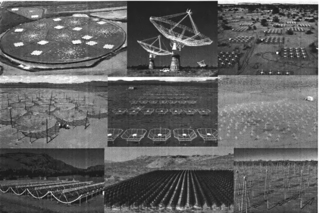
1-4 Several examples of existing and upcoming interferometry experiments pursuing a detection of cosmological 21cm fluctuations. From left to right and top to bottom: LOFAR, the GMRT, the MWA, HERA, PAPER, the LWA, CHIME, HIRAX, and the SKA-1 LOW. Several of the arrays ("imaging arrays") have their antennas distributed in a random fashion while others arrange their antenna elements in regular

patterns ("redundant arrays"). . . . . 80

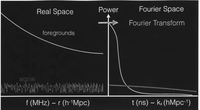
1-5 While the foregrounds in 21 cm experiments are a factor of ~ 104 times brighter, they are expected to evolve smoothly in frequency and are thus characterizable by a power law. Cosmological 21 cm emission is expected to have complex frequency structure. Thus the foregrounds and signal can be isolated by a Fourier transform in the frequency

(15)

1-6 A cartoon representation of the "EoR window" from Dillon et al. (2015b).

In the absence of instrumental effects, foregrounds would possess smooth frequency evolution and the EoR window would extend to the same

small kl for all k₁. The Fourier exponent in equation 1.8 gives rise to

the "wedge", denoted by the dark red and orange features. Chromatic-ity in the primary beam, arising from equation 1.9 adds additional contamination which is usually accounted for by a buffer denoted by

the yellow region. . . . . 83

1-7 Left: Greig and Mesinger (2017)'s estimate for the 1 - - confidence region for the evolution of the neutral fraction of the intergalactic medium as a function of redshift. Right: Greig et al. (2016)'s calcu-lation of existing limits on the spin temperature and neutral fraction the intergalactic medium at redshift 8.4 (Greig et al., 2016) including (top-left) recent 21 cm upper limits by (Ali et al., 2015), 21 cm and McGreer et al. (2015) dark-pixel statistics from high redshift quasars

(top right), 21 cm and CMB observations (bottom left) . . . . 86

1-8 All of the upper limits on the 21 cm power spectrum at the time of this

thesis between z _ 6 and z r 12. (Jacobs, Private Communication).

The sensitivity of the next generation HERA instrument is shown as

a yellow line. . . . . 87

2-1 Poisson (cosmic variance) component of the S/N, i.e. V/k, for our

fiducial observational strategy and k e 0.1 Mpc 1_. _{. . . .} ₁₀₀

2-2 Time spent in each uv cell for a 2000h observation at z = 10 for

(16)

2-3 Top panels: Amplitude of the 21cm power at k = 0.1 Mpc- 1 in var-ious models. We also plot the (1a) sensitivity curves corresponding to a 2000h observation with: MWA128T, LOFAR, SKA on the left, and MWA256T, PAPER, and the proposed HERA instrument on the right. The recent upper limit from Parsons et al. (2014) is shown at z = 7.7. Bottom panels: The corresponding average 21cm brightness

temperature offset from the CMB. . . . . 105

2-4 Various quantities evaluated at the redshift where the k = 0.1 Mpc-I

power is the largest in each model. Shown are power amplitude, red-shift, mean neutral fraction, and mean brightness temperature, clock-wise from top left. Overlaid are the Thompson scattering optical depth,

Te, contours corresponding to 1 and 2 -constraints from the 9yr release

of WMAP data (WMAP9; Hinshaw et al. 2013). The right-side y-axis

shows the corresponding values of the WDM particle mass, mwdm,

com-puted according to the approximation in eq. (2.5). Regions of the pa-rameter space in which the peak power occurs during the reionization or X-ray heating epochs are demarcated with the appropriate labels in

som e panels. . . . . 107

2-5 Cumulative distributions of T/Ts (see eq. 2.1), at z = 14,16, 18

(spanning the X-ray peak) for a fiducial, Tir = 104 K, fx = 1 model.

As seen above, the power peaks when the distribution of T/Ts is the

(17)

2-6 S/N of the detection of the k = 0.1 Mpc- 1 21cm peak power (i.e. computed at the redshift of the maximum signal). All maps show the same range in S/N to highlight differences between instruments, and are computed assuming a total integration time of 2000h. Due to our fiducial observing strategy which minimizes thermal noise at the expense of cosmic variance, some high S/N regions (S/N > 50) are limited by cosmic (Poisson) variance for the case of LOFAR and SKA, which have smaller beams than MWA and PAPER (see Fig. 2-1). This Poisson variance limit can be avoided with a different observing strat-egy; hence we caution the reader not to lend weight to the apparent better performance of MWA and PAPER in the upper left region of parameter space. . . . .111

2-7 Maximum S/N possible with current and upcoming interferometers

after 2000h (considering all redshifts instead of just the peak signal as

in F ig. 2-6). . . . 113

2-8 The S/N vs redshift evolution for the "fiducial" model, with Mmin =

108M O, fx = 1. . . . . 115

2-9 The 21cm power spectrum amplitude at k = 0.1 Mpc-- (left), 6Tb

(center), and XHI (right), all evaluated at the redshift when S/N is the

largest, assuming MWA128 sensitivities. . . . . 116

2-10 The maximum S/N for MWA-128T at k = 0.2Mpc-1. . . . . 1 18

3-1 The mean thermal evolution of our IGM simulations for our three

mod-els. "cool IGM"- solid lines, "fiducial IGM"- dashed-dotted lines, and

"hot IGM" - dashed lines. (T,) is plotted in lavendar. Varying fx

effectively shifts (T,) in redshift. . . . . 132

3-2 The 21 cm forest is dominated by sources in the 1-10 mJy flux range.

We plot the sum of fluxes squared, in Equation (3.16), for S < Sv.

A detection of Pf would constrain the high redshift source counts at

(18)

3-3 For every heating scenario we study, there is some redshift and region within the EoR window for which 21 cm forest dominates the power spectrum. Here we show the fractional difference between the power spectrum with, (P), and without (Pb) the forest for the redshifts (top to bottom) 9.2, 11.2, 12.2, 15.4, and 17.5. The diagonal lines denote

the location of the "wedge". By z > 12.2 there is a substantial region

(kjj > 0.5 Mpc-1 ) of the Fourier volume that our simulations cover in

which the forest dominates P by a factor of a few. . . . . 137

3-4 The 21 cm forest dominates the spherically averaged power spectrum

for k > 0.5 Mpc- 1. Plotted is the spherically averaged power spectrum

with (dashed lines) and without (solid lines) the presence of the 21 cm forest. In our cool model, the forest causes a significant power increase

at k > 0.5 Mpc- 1 at redshifts as low as z = 11.2. At z = 15.4 we

see a significant feature in all thermal scenarios. Our cool IGM model

experiences a reduction in the power spectrum amplitude at z > 17.5

as it passes through the X-ray heating peak. . . . . 139

3-5 We plot the magnitude of the difference between the 21 cm power

spectrum with and without the presence of the 21 cm forest including the auto-power and cross power terms of Equation (3.13). At high

redshifts and low fx, there is little k1 structure in Pl - P, indicating

that Pf is the significant contributer. At lower redshifts and higher

fx, we see signficant ki structure, indicating that in a heated IGM,

Pb - P is dominated by Pf,b which is somewhat spherically symmetric

and negative at large k. The trough in the low redshift plots marks

the region where Pf - 2Re(Pf,b) transitions from negative (for small k)

(19)

3-6 Our semi-analytic prediction agrees well with unclustered simulation results. The semi-analytic prediction of Equation (3.15) is plotted with dashed lines and A' (k) computed directly from our simulation without

clustering in solid lines. This demonstrates that for k ; 10-1 Mpc- 1_,

the cross terms in Equation (3.14) may be ignored and Pf may be

well approximated by the LoS power spectrum of T2 1 multiplied by the

summed squared fluxes for sources lying in and behind the data cube. 142

3-7 We see that for a fixed quasar distribution, the magnitude of Pf can

be parameterized by (T) and that the amplitude is consistant with a

simple power law. Here, we plot P(ki) at kl = 0.5 Mpc-1 _{vs. (T,) for}

all considered redshifts and fx. The black line is the power law (T,)-2

as one might expect for an amplitude set by (T2 1)

2 _{(Equation (3.16)).}

Inasmuch of this simple trend, a modest spread in heating models gives us a decent understanding of the behavior of the amplitude for Pj. This relation holds for the quasar population considered here because the integral over the luminosity function does not change significantly over the redshifts we consider. . . . 143

3-8 The cross power spectrum, Re(P,b)'s, sign is determined by the

anti-correlation of XHI and T, during the pre-heating epoch and by XHI

after heating has taken place. Here we show the sign of Re(Pf,b) for

our three different heating models as a function of redshift. At

pre-heating redshifts, T, is small and XHI is relatively uniform so that T

and Tf primarily depend on T, and anti-correlate so that Re(Pf,b) is

negative. At low redshifts, T is independent of T, and fluctuations are

primarily sourced by XHI so that T and Tf are correlated and Re(Pf,b)

is positive. Futhermore, heating proceeds in an "inside-out" manner so

(20)

3-9 Array layouts that we use to determine the detectibility and distin-guishability of the 21 cm forest power spectrum signature. We chose to study two moderate extensions of the MWA-128T: MWA-256T and MWA-512T. In addition we study a 4096T array that is representative of a HERA scale instrument with ~ 400 times the collecting area of the MWA. Tile locations are drawn randomly from a distribution that

is constant for the inner 50 m and drops as r-2 for larger radii. ... 148

3-10 Detections (black dots) and upper limits (red triangles) of the 21 cm

Power Spectrum at z=11.2 for all of our arrays and heating models in the presence of 21 cm forest absorption from background RL sources. The grey fill denotes the 2 - region around the measured power spec-trum with no RL sources present. To determine whether we can detect the forest imprint we ask, "do the points and their error bars lie out-side the gray shaded region?" MWA-256T and MWA-512T would be capable of distinguishing power spectra with or without sources in our cool IGM model, however only 4096T is consistantly sensitive to the

k > 0.5 Mpc' region where the forest dominates. Only for our cool

IGM model, MWA-512T would sufficient to detect this upturn as well.

Hence a moderate MWA extension would likely be able to constrain some RL populations given a cooler heating scenario while a HERA scale instrument will be able to constrain the W08 RL population using the Forest power spectrum even for more emissive heating scenarios.

Note that the upturn in the gray region is not from increased power at

(21)

3-11 These plots are identical to Figure 3-10 except the array is fixed to be

MWA-4096T, representative of a HERA generation instrument, and redshift is varied. A HERA class instrument is able to resolve the

upturn at k > 0.5 Mpc- 1 that distinguishes the forest, and should be

able to detect the 21 cm forest feature considered in this work for a variety of heating scenarios. The thermal noise error bars are to small

to resolve by eye in most of these plots. . . . . 153

3-12 The significance of distinguishability across all measured k bins

(Equa-tion (3.29)) for all arrays, redshifts, and IGM heating models for a

1000 hour observation. An extension of MWA-128T is capable of

dis-tinguishing models with and without the 21 cm forest from the W08 RL population in our cool and fiducial heating scenarios. MWA-512T and HERA scale MWA-4096T are capable of distinguishing the forest

in the power spectrum in all heating models considered in this work. . 155

3-13 The 21 cm Forest moderately enchances the distinguishability between

thermal scenarios and MWA scale interferometers can distinguish be-tween the power spectra for reasonable X-ray heating histories. Here we show the cumulative z-score described in Equation (3.29), except now applied to the difference between different IGM heating models, for all arrays and redshifts. At low redshift, the forest decreases the distinguishability of different X-ray heating scenarios by subtracting from the higher amplitude model. When the positive auto-term dom-inates at high redshift, the forest increases the contrast between given

(22)

3-14 The ratio of the 21 cm Forest power spectrum, Pf(k = 0.5 Mpc- 1) to thermal noise for 1000 hours of observation on a HERA scale in-terometer, extrapolated over a large range of X-ray efficiencies and flux squared densities. Vertical dashed black and white lines indicate the value of the simulation by (Wilman et al., 2008) while the horizon-tal black and white lines indicate the fx efficiencies that we explicitly simulate in this paper. At the highest redshifts, (T,) levels off and the detectability of the signal is independent of redshift. At late prereion-izatoin redshifts, we see that the 21 cm Forest will only be detectable for heating efficiencies < 1. . . . 158

3-15 The LoS cross power spectra between spatially separated lines of site

are on the order of - 100-1000 times smaller than auto power spectra.

In the left figure, we plot the ratio of the real cross power spectra between lines of site separated by 24 Mpc to auto power spectra, and on the right we show the ratio of the imaginary cross power spectrum

to the auto power spectrum. In both cases, for ki

>

10-1 Mpc-1, the

cross power spectra are on the order of 10-1000 times smaller. The real cross power spectrum becomes non negligible on scales comparable to

the separation between the two lines of site. . . . . 165

3-16 Here we see that P[Ecross(ui, 0, N) is invariant in N,

E,

and u1 ,

and N with a mean of approximately zero. The lines which indicate,

P[EcrO,(ui, E, N)], are estimated from 10000 draws. Since (Ecross) ~

0 we expect the cross terms to contribute negligibly to Pf in 3D Fourier

(23)

3-17 Left: The percentage of the integrated luminosity function in Equation (3.16) as a function of the source fluxes at 5GHz for comparison to the

catalogue of H04. We see that most contributions to the forest power

spectrum come in between S5 GHz = 10 pJy and S5 GHz = 10 mJy.

Right: The ratio of the number of sources with redshift greater than

z between S5 GHz = 10 pJy and 10 mJy as predicted by the W08 and

H04. The W08 simulation over predicts the counts in H04 by a factor

ten at z > 12 and nearly 80 at z > 16, emphasizing the importance of

exploring this widely unconstrained parameter space in future work. . 170

4-1 Top: The evolution of the density weighted average of the neutral

fraction. Middle: The evolution of the kinetic temperature (T), Ts,

Tcmb. Bottom: the redshift evolution of the mean 21 cm brightness

temperature, (6Tb). All averages are taken over volume. . . . . 182

4-2 A2 as a function of redshift for two different Id k bins, k = 0.lhMpc-1

(black lines) and k = 0.4hMpc-1 (red lines). For each parameter, we

show the power spectrum at 6 = 0.1 (thick solid and thick dashed

lines respectively) along with the difference (thin solid lines). Note that our parameterization defines 0 as the fractional difference of each parameter from its fiducial. The first two peaks of the three-peaked structure, discussed in Pritchard and Furlanetto (2007); Santos et al.

(2008); Baek et al. (2010) and Mesinger et al. (2013), is clearly visible

representing the epochs of reionization and X-ray heating. With the exception of Rmfp, parameter changes affect a broad range of redshifts. 184

(24)

4-3 Top: The power spectrum of 21 cm fluctuations (solid red lines) over numerous redshifts. Filled regions denote the l- errors for the instru-ments considered in this paper with moderate foregrounds. Bottom: The derivatives of the 21 cm power spectrum with respect to the as-trophysical parameters considered in this work as a function of k at various redshifts. Derivatives are substantial over all redshifts except

for Rmfp which only affects the end of reionization. Notably, CA21 is

negative on small scales at high redshift, a signature of the beginnings of inside out reionization while X-ray spectral parameters follow very

similar redshift trends, indicative of degeneracy. . . . . 189

4-4 Left: The logarithm of the probability distribution function (PDF)

of pixels at z = 12.4 for our fiducial model as a function of T, vs.

XHI. Even before the majority of reionization, early HII bubbles ionize

the hottest points in the IGM, leading to a pileup of high T, pixels at XHI = 0 and reducing the contrast in JTb between hot and cold

regions. Right: PDFs of 6Tb with and without XHI manually set to

unity everywhere. The presence of ionization during X-ray heating leads to a decrease in the large T, wing, near 30 mK, and a spike at

0 mK, leading to a reduction in the dynamic range of the field and an

overall decrease in power . . . . 191

4-5 Plotting wi (k, z) versus redshift for several different co-moving scales

gives us a sense of the covariances between various parameters. Here we assume 1080 hours of observation on HERA-331 and the moderate

foreground model. Since the thermal noise on A increases rapidly

with k, wi is maximized at larger spatial scales. As we might expect

from our fiducial model, wi for reionization parameters is maximized

at lower redshifts while wi for X-ray spectral parameters is significant

over the heating epoch. Trn affects both heating and reionization and has a broad redshift distribution. Vertical lines indicate the location

(25)

4-6 Plotting wi(k, z) at a single cosmological Fourier mode for all of our parameters on the same panel facilitates direct comparison. Many of the parameters have similar redshift evolutions that differ by a sign,

making their effects on the power spectrum degenerate. . . . . 195

4-7 The fractional errors on astrophysical parameters as a function of max-imal observed redshift for HERA-331 with moderate foreground tamination. From low redshift measurements, vmin and fx are con-strained to within ~ 40%t hough the spectral index ax remains highly

uncertain. Measurements at z > 10 allow for < 10% limits on X-ray

spectral parameters, including cex and a factor of two improvement in constraints on Tii" and reionization. Inability to observe within the FM radio-band (pink shaded region) raises the errors on heating pa-rameters by a factor of two. The fall of the error bars with redshift

bottoms out at high z due to increasing thermal noise. . . . . 196

4-8 95% confidence regions for the X-ray spectral properties of early

galax-ies, marginalizing over ((, Rmfp, Ti" from measurements on

HERA-331 with our moderate foregrounds scenario. At low redshift (z < 10),

hardly any signature of ax is present, leading to large error bars on

the ax axis. Because Vmin and fx incur very similar changes on the

power spectrum during the beginning of reionization (Fig. 4-5), they are highly degenerate. Observations of the heating peak break these

(26)

4-9 Confidence ellipses (95%) for Tmr and reionization parameters. By comparing the ellipses resulting from fixing our heating history and only observing at low redshift and the ellipses resulting from marginal-izing over all parameters but including heating epoch measurements, one can see that a significant fraction of the gains in reionization uncer-tainties at high redshift come from breaking degeneracies with heating parameters rather than the direct signatures of reionization. This also shows that not marginalizing over heating parameters leads to

over-optimistic predictions of reionization uncertainties. . . . . 199

4-10 95% confidence ellipses for our moderate and optimistic foreground models assuming 1080 hours of drift-scan observations on HERA-331. Heating parameters tend to be highly degenerate with eachother but independent of reionization parameters. As the majority of the in-formation heating comes from higher redshifts where thermal noise is much higher, their uncertainty regions tend to be several times larger. 204

5-1 A radio map at 408 MHz (Haslam et al., 1982) sin-projected over the

region of the sky observed in this paper. Cyan through magenta con-tours indicate the total fraction of observation time weighted by our primary beam gain for our three hours of observation at 83 MHz. Red contours indicate R.A.-decl. lines. Observation tracked the position

(R.A.(J2000) = 4h0'm0s, decl.(J2000)=-30 0'0") on a region of the sky with relatively little galactic contamination and dominated by the resolved sources Fornax A and Pictor A. The galactic anticentre and bright diffuse sources, such as the Gum Nebula, are below 1% bore-site

(27)

5-2 The autocorrelation spectrum of a single tile, showing the MWA

band-pass, is plotted here (solid black line) along with the frequency ranges over which our data was taken (gray striped rectangles). Observations were performed simultaneously on two non-contiguous bands located on either side of the 88-108 MHz FM band (red shaded region) to both assess conditions within the FM band and to preserve some usable bandwidth should it have proven overly contaminated by RFI. . . . . 212

5-3 A false-color plot of the fractional change in our calibration amplitudes

over each pointing (in which beamformer delay settings are fixed). Pointing changes are marked by the solid white horizontal lines. We see that the calibration amplitudes vary within a pointing on the order of several percent with little systematic variation. There are several coarse channel scale jumps on September 5th that correspond to ob-servations in which the number of sources identified within a snapshot image were reduced (see Fig. 5-9). We found that these jumps corre-sponded to excess flagging from cotter, indicating high levels of RFI or other bad data, and dropped them from our analysis. Vertical lines from RFI are visible at 98 MHz and 107 MHz, especially on September

6th . . . . . 2 15

5-4 A deep image of the MWA "EoR-01" field centered at (R.A.(J2000) =

4 h 0 0s ' and decl.(J2000)=-300'0"), derived by stacking restored mul-tifrequency synthesis Stokes XX and YY images produced by WSClean on Band 1. The dominant source in our field is Fornax A (detailed in the inset) whose structure is well recovered in imaging. Pictor A is

also present at the center of the image (at - 30% beam) along with

(28)

5-5 Left: The standard deviation over uv cells as a function of frequency for an even/odd time step difference cube after three hours of integration. The blue line is derived from data, while the green line is a model with a system temperature of 470 K at 150 MHz and a spectral index

of -2.6. Spikes in the standard deviation are present at the center

of each coarse channel since the center channel has one half of the data due to flagging the center channel which is contaminated by a digital artifact before averaging from 40 to 80 kHz. Right: The ratio of variance taken over frequency in each uv cell and our variance model using the same system temperature as on the left. The ratio between our model and observed variance is close to unity across the uv plane. White cells indicate uv voxels that were flagged at all frequencies due

to poor sampling. All data in this figure is from Band 1. . . . . 224

5-6 The percentage of visibilities flagged for RFI by cotter as a function

of time and frequency. White regions indicate missing data including the coarse band edges and blue-dashed vertical lines indicate the edge of the FM band. While Band 1 remains predominantly clear with a few sparse events within the lower end of the FM band, contamination is significantly greater over Band 2. Even in the FM band, RFI events are either isolated in frequency or time, allowing us to flag them. A handful of observations in Band 1 on September 5th are missing entire coarse channels which we also discard. Bar plots on the bottom and right show the averages of the RFI flagging fraction over time and

(29)

5-7 Differential refraction derived from source pairs within 30 minute bins

on September 5th, 2013 (top row) and September 6th, 2013 (bottom row). Band 1 (black points) scaled by the ratio of the band center fre-quencies square (solid black line) very nicely predicts the differential refraction in Band 2 (red points), indicating that the refraction we are measuring here is indeed due to ionospheric fluctuations. The magni-tude of ionospheric activity differs significantly between September 5th and 6th and peaks over the last observations taken on the 6th. We also show fits to an isotropic power spectrum model of differential refraction

at 83 MHz (dashed black line) and print the inferred diffractive scale. 232

5-8 The dimensionless integral, F, (x) normalized to unity at F,,(10), given

in equation 5.20. For small values of x, F,(X) is well approximated

by a power law, but flattens out towards x = 1. Hence, the

struc-ture function of observed source offsets levels out at the outer energy

injection scale of the turbulence. . . . . 232

5-9 The number of sources identified in 112s multifrequency synthesis

im-ages of Band 1 as a function of time over both nights of observing. On September 5th, the source counts increase with primary beam gain,

until transit (vertical gray line

)

before decreasing. On September

6th, when more severe ionospheric refraction was observed, the source counts remain significantly lower. Fewer sources were identified in a handful of September 5th snapshots corresponding to observations in which calibration and flagging anomolies were observed ( Figs. 5-3 and

(30)

5-10 The regions of the EoR window contaminated by foregrounds due

to uncalibrated cable reflections for several different redshifts. Dark gray regions denote contamination from first order cable reflections assuming a wedge out to the first null of the primary beam plus the

0.15 h Mpc1 at z = 8.5 buffer observed in Pober et al. (2013a). Since

the buffer is associated with the intrinsic spectral structure of fore-grounds, it lives in delay space. Dark gray regions denote foreground contamination within the wedge which exists even without

instrumen-tal spectral structure. At z = 7, a representative EoR redshift, the

contaminated regions remain at relatively high kl and have smaller

widths due to the smaller primary beam and the scaling of k1 and

k1l with z. While regions exist between the first order reflections that

are somewhat wider at lower redshift, second order reflections can still potentially contaminate nearly all of the EoR window in which inter-ferometers are supposed to be sensitive (light grey shaded regions). Second order reflections are below the sensitivity level of this study but will also pose an obstacle to longer integration unless calibrated out.239

5-11 We show the amplitude of a calibration gain averaged over a fifteen

minute pointing (black circles) along with the square root of our auto-correlations which have been scaled by a third order polynomial and a single seven meter reflection to match the calibration solution (red line). After multiplying the autocorrelations by a smooth function,

they are brought into good agreement with the calibration gains. . . . 242

5-12 Left: In order to obtain reflection parameters, we divide our scaled

autocorrelation (magenta circles) by a smooth fuction consisting of a third order polynomial and large scale reflections (green line). Right: We fit this ratio (magenta circles) to a reflection function (green line)

(31)

5-13 Histograms of fitted cable reflection amplitudes for Band 1 (blue) and

Band 2 (green) obtained from fits to autocorrelations for three dif-ferent cable lengths between MWA receivers and tiles. The reflection

amplitudes range from 0.2 - 1% making them difficult to fit using the

noisy self calibration solutions. Reflection amplitudes in Band 2 are systematically larger than Band 1 for all cable lengths, indicative of

non-trivial frequency evolution in the reflection parameters . . . . 244

5-14 Dynamic spectra of the square root of a representative tile autocor-relation. Note the different color bars for the two frequency bands since Band 1 evolves more steeply in frequency than Band 2. The au-tocorrelations exhibit repetitive structure in time from night to night with smooth time variations occuring as the sky rotates overhead and steep transitions occuring every ~ 30 minutes due to changes in the analogue beamformer settings as the antennas track the sky. Limited RFI is plainly visible within the FM band, especially in Band 2, and the events are consistent with the flagging events identified by cotter

shown in Fig. 5-6. . . . . 245

5-15 Left: The residuals to fitting reflection functions in our

autocorrela-tions for all two minute time-steps in our analysis for a representa-tive tile with a 90 meter beamformer to receiver connection (light grey points). While some scatter exists in the residuals due to fitting noise,

they average to non-zero values on the order of - 10-' (black dots).

These residuals are due to mismodeling the reflections and at a lower level potentially arise from digital artifacts. Right: The same as the left

but for a 150 meter cable whose reflection coefficient is - x 2 as large

(32)

5-16 The absolute value of our cylindrical power spectrum estimate from

our three nights of observing on Band 2 (left) and Band 1 (right). We overplot the locations of the primary beam (dash-dotted), horizon (dashed), and horizon plus a 0.1 h Mpc-' buffer (solid black) wedges. We see that the foregrounds are primarily contained within the wedge and that the EoR window is, for the most part, noise-like. There is

some low SNR structure below k11 ~ 0.5 h Mpc-', corresponding to kl

modes contaminated by cable reflections. The amplitude in power rises very quickly due to an increase in thermal noise which rises very quickly

at large k11 due to a rapid falloff in uv coverage beyond k1 ~ 0.2 hMpc 1.249

5-17 P(k) over Band 2 (left) and Band 1 (right) with a color scale that

high-lights cells with positive or negative values. We expect regions that are thermal noise dominated to contain an equal number of positive and negative estimates and regions that are dominated by foreground leakage to be entirely positive. We observe significant foreground

con-tamination outside of the wedge up to ki 0.5 h Mpc-1 in both bands. 250

5-18 The errors on ' arising from residual foregrounds and thermal noise are

determined by looking at even/odd difference cubes and foreground-subtracted residual cubes using the method of Dillon et al. (2015a). We show the error bars on our cylindrical power spectrum here, seeing that errors arising from foregrounds are contained within the wedge. These

foreground errors are maximized at the smallest and largest k1 arising

from large power in diffuse emission and increasing thermal noise from

(33)

5-19 The foreground contamination within the wedge along with residual

detections due to miscalibrated fine frequency features in the bandpass are especially clear in plots of the ratio between power and the error bars estimated by the empirical covariance method of D15. We overplot

the wedge with a 0.1 h Mpc- 1 _{buffer along with the wedge translated}

to cable reflection delays of our 90 and 150 m receiver to beamformer

cables to highlight the effect of this systematic. . . . . 252

5-20 Here we show the ratio between our 2D power spectrum and the

er-ror bars estimated by the emprical covariance method of Dillon et al. (2015a). On the top left, we show our data calibrated using our initial

calibration (see 5.2.2) with no attempt made to correct for standing

wave structure in the MWA bandpass. Bright, band-like structures are clearly visible at the delays associated with reflections. On the top right, we show a first attempt to correct for cable reflections by fitting a sinusoidal model to rather noisy calibration solutions that had been integrated over a night of observing (1.5 hours each night). While the bands appear weaker, they are still quiete visible above the noise. In the bottom right panel, we show the same plot with calibration

solu-tions using scaled autocorrelasolu-tions described in 5.3.4. In the lower

left panel we show a power spectrum with calibration solutions using autocorrelations for the amplitudes but without any attempt to cor-rect reflections in the phase solutions. Pronounced reflection features are visible in this power spectrum, indicating that any mismodeled

(34)

5-21 The level of power at a fixed kII corresponding to the delay of

reflec-tions from our 150 m cable (left), and comparing it to a value of k1

unaffected by cable reflections (right). The blue line shows the power spectrum level for calibration in which the bandpass is modeled as a polynomial with no attempt to correct fine frequency scale reflections. We see that power is on the order of ~ 50 times the thermal noise level (green-dashed line). Attempting to fit the reflections to calibra-tion solucalibra-tions integrated over each night gives us an improvement in the power level by roughly an order of magnitude (orange solid line). Using calibration solutions derived from autocorrelations brings down the reflection power by another factor of a few (purple solid line) but is still unable to bring the majority of measurements below the ~ 1-level. While we think that the autocorrelations accurately capture the fine frequency structure of the gains, we are still forced to model this fine frequency structure and predict it in the phases. Residual power is likely due to inaccuracies in this modeling. The right hand panel shows all data below the stimated noise level. This is due to the fact that in (Dillon et al., 2014) it is shown that the method for calculating error bars layed-out in Liu and Tegmark (2011); Dillon et al. (2013) slightly over-estimates the noise. . . . 256

5-22 The Band 1, Id power spectra from our two nights of observing:

Septem-ber 5th, 2013 (black) and SeptemSeptem-ber 6th, 2013 (red). We saw in Fig.

5-7, that the magnitude of refractions on September 6th were on average

twice as severe. The two power spectra nearly indistinguishable (within error bars) despite the significant differences in conditions, indicating that ionospheric systematics do not have a significant effect after three hours of integration, even at these low frequencies. . . . 258

(35)

5-23 Dimensionless 1d power spectra derived by Integrating spherical shells

excluding the foreground contaminated wedge region with a 0.1 h Mpc- 1

buffer. Black dots indicate the mean estimated from the weighted av-erage in each bin. Vertical error bars denote the 2- uncertainties while horizontal error bars indicate the width of window functions. We also shade regions of k-space that we expect to have some level of fore-ground contamination due to uncalibrated cable reflection structure. Gray shaded regions clearly correspond to regions in which our power spectrum measurements are not consistent with thermal noise. We note that where our upper limits do agree with thermal noise, the

power spectrum is on the order of - 100 times larger than the upper

limits set with the MWA at ~ 180 MHz(D15). This factor is reasonable

given that the sky noise (noise power spectrum) scales with ~

f-2.-(f

5 2

₎

_{and the primary beam solid angle increases as} _~_{f2 . . . .} 260

6-1 The HERA antenna element (bottom) uses a parabolic dish to achieve

an order of magnitude increase in collecting area over the PAPER an-tenna (top). The sleeved dipole in the center of the PAPER backplane is identical to the sleeved dipole being suspended under the cylindrical skirt over the vertex of the HERA dish. The suspended feed arrange-ment has the potential to introduce intra-antenna reflections which we

(36)

6-2 A cartoon demonstration of the impact on foregrounds of the frequency

dependent beam. Left: The location of three, spectrally flat, sources in delay space assuming a frequency independent beam (no reflections in the antenna element). Right: the presence of chromaticity due to delayed signal within the antenna smears the source in delay with the kernel given by equation 6.7. Since the frequency response of the dish is a function of direction on the sky, the shape of the delay kernel is different for each source line. We see that this smearing can lead to sub-stantial supra-horizon emission. In this paper, we consider a direction independent delay-kernel that is source primarily by reflections while a more general direction-dependent kernel is explored in Thyagarajan

et al. (2016) . . . . 280

6-3 An illustration of our simulation products and their origin in the HERA

antenna geometry. A plane wave is injected from above the feed. The electric field of the plane wave at the feed terminals (red line) along with the voltage output is recorded (black line). The feed in our simulation is situated 5 m above the bottom of the dish, hence there is a ~ 30 ns delay between when the plane wave passes the terminal for the first time (A) and when it is first absorbed in the dipole (B), leading to the voltage response. Of concern to 21 cm experiments are the subsequent reflections between the feed and the dish (C) which can lead to larger

(37)

6-4 The absolute value of the Fourier transform of the voltage output from our dish simulations (green line) and the input wave (blue line), nor-malized to the amplitude of the input wave at 150 MHz. The ratio between input and output is plotted as a red line. Since our input is limited to frequencies between ~ 20 and 280 MHz, there are significant numerical artifacts in the ratio that causes divergence towards the plot edges. To eliminate this noise, we multiply by a Blackman-Harris win-dow between 100 and 200 MHz and set our estimate to zero elsewhere

(cyan line). . . . . 284

6-5 The Fourier transform of the simulated voltage response of the HERA

Dish (solid black line) and the PAPER antenna element (dashed black line). Reflections in the HERA dish element lead to significantly

en-hanced power above - 50 ns. Since negative delays should be devoid of

signal, they allow us to determine the dynamic range of our simulations which have a numerical noise/sidelobes floor of -60 dB. . . . 286

6-6 The absolute value of the power kernel for the HERA dish (solid black

line) and for the PAPER antenna element (dashed black line) calcu-lated using equation 6.7. While an antenna can only physically have a voltage response at positive delays, the delay kernel is formed from the convolution of one antenna with the time reversed conjugate re-sponse function of the other. Hence, the power kernel for two identical

(38)

6-7 The power kernel for the three subbands discussed in 6.4.2 along with the kernel for the full bandwidth response function. While the

long term falloff from reflections is prominent between 130 - 160 MHz,

it appears at a much lower level in the other two subbands which fall

below the central subband by - 20 dB at - 300 ns. k₁₁values for

each delay are computed at 150 MHz. The wider central lobe below

150 ns for the subband gains is due to the lower delay resolution from

the smaller bandwidth. We also show the delay kernel for 100 MHz

bandwidth (black thick line) . . . . 288

6-8 Residuals on the absolute value of the gain over several subbands after

fitting to a sixth order polynomial. Consistent with our findings in Fig. 6-7, the fine frequency residuals in the 145-155 MHz subband are

over an order of magnitude greater than those in the other subbands. 288

6-9 A closeup rendering of the HERA feed which is suspended over the

re-flector, illustrating the cylindrical skirt, the backplane, and the dipole. Long time-scale spectral structure arises from electrical oscillations

within the cylindrical cavity. . . . . 290

6-10 The absolute value of the time-domain voltage response of the

cylindri-cal dipole feed compared to the absolute value of the voltage response of the feed suspended over the dish. As we might expect, the ~ 35 nm lobed structures associated with feed-dish reflections are absent from the simulation of the feed only. However, the knee like feature after ~ 100 ns is. This indicates that the most severe spectral contamination in the current HERA design does not originate in reflections between

(39)

6-11 The time-domain response of the HERA antenna towards a plane wave

incident from zenith for a variety of termination impedances. As we vary the termination impedance, the structure which is dominated by feed-dish reflections, below ~ 150ns, varies significantly but leaves de-lays greater than ~ 200 ns unchanged. Only in the extreme, 500 Q case do the reflections extend to large delays. Since structure above 250 ns is primarily reponsible for contaminating the EoR window (6-14), the termination impedance has a relatively small impact on HERA's

over-all sensitivity. . . . 291

6-12 A comparison between time-domain simulations (black line) and

mea-surements (grey line) of S₁₁ for the HERA dish. We also show an

S11 measurement with the cables leading from the VNA to the feed

terminated by an open circuit which allows us to probe the dynamic range of the measurement. We use the standard deviation of the open measurement (grey dashed line) between 200 and 400 ns as our system-atic floor (grey shaded region). We find very good agreement between our Si measurement and the simulation, validating the predictions of our simulations. Both the simulations and measurements in this figure

(40)

6-13 The absolute magnitude of a 100-200 MHz delay transformed visibility

from a 14-meter baseline (blue line) compared to the same visibil-ity (green line) contaminated by the delay-response observed in our simulations of the HERA dish. We see that the extended delay ker-nel smooths out structure, originating from foregrounds, within the horizon. For HERA, we expect to use the delay-CLEAN to remove foregrounds. However, the depth of CLEANing is limited by the noise level on a single baseline. We show the foreground residuals from a

CLEAN down to the 5 o noise level after 20 minutes of integration. Since CLEANing cannot distinguish between foregrounds and signal, it should only be performed within a narrow region of delay-space, close to the horizon and cannot remove the broad wings leaked by the