Approximation Algorithms for
Survivable Network Design
Doctoral Dissertation submitted to the
Faculty of Informatics of the Università della Svizzera Italiana in partial fulfillment of the requirements for the degree of
Doctor of Philosophy
presented by
Afrouz Jabal Ameli
under the supervision of
Prof. Fabrizio Grandoni
Dissertation Committee
Prof. Jaros≥aw Byrka University of Wroc≥aw
Prof. Antonio Carzaniga Università della Svizzera Italiana, Switzerland Prof. Stefano Leonardi Università “La Sapienza” Roma, Italy
Prof. Stefan Wolf Università della Svizzera Italiana, Switzerland
Dissertation accepted on 19 April 2021
Research Advisor PhD Program Director
Prof. Fabrizio Grandoni Prof. Walter Binder / Prof. Silvia Santini
I certify that except where due acknowledgement has been given, the work presented in this thesis is that of the author alone; the work has not been sub-mitted previously, in whole or in part, to qualify for any other academic award; and the content of the thesis is the result of work which has been carried out since the official commencement date of the approved research program.
Afrouz Jabal Ameli Lugano, 19 April 2021
To my family
In the name of God.
Abstract
Many relevant discrete optimization problems are believed to be hard to solve
efficiently (i.e. they cannot be solved in polynomial time unless P=NP). An approximation algorithm is one of the ways to tackle these hard optimization
problems. These algorithms have polynomial running time and compute a fea-sible solution whose value is within a proven factor (approximation factor) of the optimal solution value. The field of approximation algorithms has grown quickly over the last few decades, leading to the development of several algo-rithmic and analytical techniques.
In this doctoral dissertation, we focus on Survivable Network Design prob-lems, where the goal is to construct low-cost networks that are resilient to a few edge/node faults. More specifically, we consider a basic problem in this area, that is the Connectivity Augmentation problem (CAP). In this problem, we are given a k-edge-connected graph (namely, a graph in which removing any
k≠ 1 edges preserves the connectivity of the graph) and a collection of extra
edges (links). Our goal is to identify a minimum cardinality subset of links whose addition to the graph makes it (k + 1)-edge connected. This problem is NP-hard and has many interesting real-world applications; For this reason it has been studied through the lens of approximation algorithms in the past.
Despite the efforts of several researchers, no progress was made on this problem after the 2-approximation algorithm by Frederickson and JáJá [1981]. We remark that a 2 approximation is known even for wide generalizations of CAP. The main contribution of this thesis is breaching the 2 approximation barrier for CAP by presenting a 1.91 approximation algorithm. Our result is based on a non-trivial reduction to another fundamental problem, Steiner Tree. Along the way to this main achievement, we studied a special case of CAP, the Cycle Augmentation problem (CycAP) for which 2 was the best-known approximation factor. Here we are given a cycle plus additional links, and the goal is to find a subset of links with minimum size whose addition to G makes it 3-edge-connected. We show that CycAP is APX-hard, in particular it does not admit an approximation factor arbitrarily close to 1 (even the
viii
hardness of this problem was not known earlier). Furthermore, we present a 3/2 + ‘ approximation algorithm for any constant ‘ > 0.
Acknowledgements
.
I want to express my gratitude to my advisor, Fabrizio Grandoni. It has been a real privilege being a student of Fabrizio. His profound knowledge of approximation algorithms and combinatorial optimization is combined with in-quisitive curiosity and a generous attitude. Besides several intriguing ideas that motivated all results of the thesis substantially, I could learn the importance of a deeper understanding of problems from him. Also, his uncompromising aesthetic standards concerning the clarity and simplicity of proofs and presen-tation have had a great impact on me. His constant search for intuitive and simple explanations, together with his thirst for knowledge and attention to detail, have set a role-model for me.
A Special thanks to Mohammad Pishnamaz, Mohammad Ali Aabaam, Alireza Alipour, Farhad Shahmohammadi and all the tutors of the Iranian Olympiad in Informatics, who initiated my interest in algorithms and discrete mathematics.
I am extremely grateful to my wife, because of her support during these years. We both suffered from being separated due to visa issues.
I am thankful to my family and friends from Iran, who constantly provided emotional support and encouragement to accomplish my projects, despite the physical distance separating us. Thanks a lot in particular to my mother Mahnaz, my father and my brother.
Thank you to all my colleagues and coauthors. It was a pleasure and honor to collaborate and share enjoyable time: Waldo Gàlvez, Kamyar Khodamoradi and Mohit Garg among others.
Special thanks to all the friends I met at IDSIA and USI, specially to my teachers and classmates at the sport groups. I would also like to thank Daniela, Cinzia and Elisa who helped me a lot to settle down in Lugano.
To all of you, my sincere gratitude.
Contents
Contents xi
1 Introduction 1
1.1 Approximation algorithms . . . 2
1.2 Lower bounds and Approximation Preserving Reductions . . . . 3
1.3 Survivable Network Design Problems . . . 5
1.4 Publications and Manuscripts . . . 7
1.5 Our results and Outline of the Thesis . . . 8
2 Preliminaries 11 2.1 Edge-connectivity . . . 11
2.2 From CAP to TAP and CacAP . . . 12
2.3 Related Problems . . . 15
3 The Cycle Augmentation Problem 19 3.1 Definitions and Notations . . . 21
3.2 Approximation algorithms . . . 24
3.3 Hardness of Approximation for CycAP . . . 32
3.4 Hardness of Approximation for WCycAP . . . 38
3.5 LP Relaxations for CycAP . . . 38
4 The Cactus Augmentation Problem 45 4.1 Steiner Tree and Connectivity Augmentation . . . 46
4.1.1 Steiner Tree via Iterative Randomized Rounding . . . 50
4.2 An Improved CacAP Approximation Algorithm . . . 51
4.2.1 An Alternative Marking Scheme . . . 52
4.2.2 Analysis of the Approximation Factor . . . 54
5 Conclusions 59 5.1 Open Problems . . . 59
xii Contents
A Details of the Steiner Tree Approximation Algorithm of Byrka
et al. [2013] 61
A.1 Witness Tree and Witness Sets . . . 63
B Omitted Proofs from Section 4.2 67
Chapter 1
Introduction
Many of the problems that we need to solve in practice are discrete optimization problems. In these problems we need to identify, among a discrete set of feasible solution, a solution which optimizes a given objective function. This captures several applications as for example deciding inventory levels, assigning tasks, organizing data for efficient retrieval etc. Unfortunately, many natural discrete optimization problems are difficult to solve efficiently (i.e., in polynomial time in the input size). In particular, assuming that P ”= NP, it is impossible to provide an algorithm that is efficient and at the same time computes the optimal solution. Yet, for several reasons these problems require more progress; (1) First of all, these problems have industrial applications that can not be ignored. (2) Researchers are curious to know what can be achieved, if an efficient exact solution is impossible. (3) Also the recent advances in hardware systems inspire that someday even semi-efficient algorithm can have better performances. Thus, an extensive research has been devoted to techniques to deal with NP-hard problem while relaxing either optimality or efficiency. This has lead to the birth of several sub-fields of algorithms and computations.
One line of research, known as Parameterized algorithms, aims for algo-rithms whose running time depends in a super-polynomial way not on the entire input size, but only on the size of a proper part of the input called parameter.
Definition 1 (Cygan et al. [2015]). A parameterized optimization problem P
is called Fixed-Parameter Tractable (FPT) if there exists an algorithm A , a computable function f : N æ N and a constant c such that, given an instance
(I, k), algorithm A correctly solves the problem in time bounded by f(k) · |I|c. Some commonly used parameters are the size of the solution, the dimension
2 1.1 Approximation algorithms
for geometrical problems and the maximum degree or the treewidth of the input graph.
A different approach to attack these problems is to consider restricted in-stances. For instance, many graph optimization problems have been studied specifically for planar or sparse graphs. In many cases this approach led to im-proved algorithms for the general case or to a deeper understanding of hardness of the problem. Moreover, for many industrial application solving restricted instances is sufficient. For instance in most real-world applications the input graph is usually sparse.
Another approach is to use approximation algorithms (Knuth [1974]), which is our main focus in this doctoral dissertation. These are polynomitime al-gorithms that compute feasible solutions of cost within a given factor
(approx-imation factor or approx(approx-imation ratio) from the value of the optimal solution.
1.1 Approximation algorithms
In this section, we introduce some fundamental definitions and concepts in the field of approximation algorithms.
Definition 2 (Knuth [1974]). Given an optimization problem P , an –-approximation
algorithm for P is an algorithm with polynomial running time that, for each
instance of the problem, outputs a solution whose value is within a factor – of the value of an optimal solution.
The approximation ratio – Ø 1 of an approximation algorithm is defined as
max IœI max
I
OPT(I)
APX(I),APX(I)OPT(I)
J
,
where I is the set of instances of the problem, APX(I) is the value of the solution computed by the approximation algorithm when run on instance I and OPT(I) is the value of an optimal solution for instance I. Ideally, – is a constant (i.e not dependant on the size of the input) and in this case we say that our algorithm is a constant approximation. Indeed in terms of optimality, the goal is to minimize –. For an NP-hard optimization problem, the best kind of approximation algorithms one can hope to design are called Polynomial Time
Approximation Schemes which we proceed to define:
Definition 3. A Polynomial Time Approximation Scheme (PTAS) for
3 1.2 Lower bounds and Approximation Preserving Reductions
each Á > 0, AÁ is a (1 + Á)-approximation algorithm for P . The running time
of these algorithms is polynomial in the input size for any fixed Á.
The class of problems that admit a PTAS and the class of problems that admit constant factor approximation are called PTAS and APX, respectively. Clearly, all problems that admit a PTAS are in APX, but the converse is not true if P ”= NP.
1.2 Lower bounds and Approximation Preserving
Reductions
For an NP-hard optimization problem P , the main challenge is to find the best possible approximation factor (–ú). Any –-approximation algorithm for P , by
definition, provides an upper bound on the best possible approximation factor (i.e this shows that –ú Æ –). A significant amount of research has been devoted
to a dual kind of result, that is, proofs that certain approximation ratios are not possible (under the assumption that P ”= NP or analogous assumptions). These results provide a lower bound on the approximation factor.
Definition 4. A problem A is called APX-hard if it does not admit a PTAS
unless P = NP .
Thus, being APX-hard is considered as a strong evidence that the problem does not admit a PTAS. For many problems, stronger lower bounds are known that rely only on the assumption that P ”= NP. For instance, a (3
2 ≠
‘)-approximation algorithm of Bin Packing Problem for any ‘ > 0, can be used to solve the Partition problem in polynomial time. In the case of the Steiner Tree problem, it is NP-hard to find a solution of size less than 96
95 of the optimal
solution. Thus the existence of a (96
95 ≠ ‘)-approximation for any ‘ > 0 seems
impossible (Chlebík and Chlebíková [2008]).
Definition 5. We say that – is a lower bound on the approximability of A, if
for any constant ‘ > 0 a polynomial time (– ≠ ‘)-approximation is impossible for A, unless P = NP .
There are many optimization problems that are hard to approximate even with a constant approximation ratio. For instance, the set cover problem can not be approximated within a factor o(log n), where n is the size of the uni-verse.
4 1.2 Lower bounds and Approximation Preserving Reductions
From the approximation algorithms perspective, the ultimate goal for any NP-Hard optimization problem is to find an approximation algorithm for it plus a matching hardness of approximation result.
In order to investigate the inapproximability of a problem A, a standard tech-nique is to use some special types of approximation-preserving reductions from other problems. More specifically, an approximation-preserving reduction from a problem A to a problem B shows that if there exists an –-approximation for
B, we can then get an f(–)-approximation for A, where f is some function.
Then we know that if A is hard to approximate within some factor x, then B is hard to approximate within a factor f≠1(x).
Figure 1.1. The diagram describing the relation of classification of NP-hard in
terms of approximability.
There are several different types of approximation-preserving reductions. Here we define only those that are used in this thesis. Strict reduction is the simplest type of approximation-preserving reduction. In a strict reduction,
f(x) = x for any x > 1, and hence the approximation ratio obtained for
problem A is at least as good as the approximation ratio of problem B. Strict reduction preserves membership in both PTAS and APX (See Lemma 14 for an example of strict reduction).
Another common type of approximation-preserving reduction are the S-reductions, for which the cost of the optimal solution for the corresponding
5 1.3 Survivable Network Design Problems
instances of A and B must have the same size. S-reduction is a very special case of strict reductions. In effect, the two problems A and B must be in near-perfect correspondence with each other. The existence of a S-reduction implies not only the existence of a strict reduction but every other approximation-preserving reduction.
In order to show that a problem B does not admit a PTAS using an APX-hard problem A, a special type of reductions known as L-reduction is required from A to B. with a L-reduction, an –-approximation for problem B is trans-formed to a (1 + a(– ≠ 1))-approximation for A, where a > 0 is a constant. Hence if A admits a PTAS, then so does B. (See section 3.3 for an example of such reductions).
For any NP-optimization the main challenge is to tighten the gap between the lower bound and upper bound of approximability. For many NP-hard problems this gap is already closed. For instance the Knapsack Problem is NP-hard and admits a PTAS. On the other hand there are many problems that still require substantial progress.
1.3 Survivable Network Design Problems
The goal of Network Design is to design cheap networks that support a given traffic. Among these problems, Survivable Network Design problems received a lot of attention in the last few years. The basic goal here is to construct low cost networks that preserve the connectivity between given sets of nodes despite the failure of a few edges/nodes (in the following we will focus on the edge failure case). This has many applications, e.g., in transportation and telecommunication networks. Several such problems are NP-hard, and in most cases the best known approximation factor is 2 due to Jain [2001].
An interesting family of survivable network design problems are the Network
Augmentation problems. Here we are given an existing network plus a collection
of extra edges (links) that can be added to the network at a given cost. Our goal is to identify a cheap subset of links whose addition to the network increases its connectivity in a desired manner. A well-studied classical problem in this area is the Connectivity Augmentation problem (CAP). Recall that a graph G is k-edge-connected (or k-connected for short), if G remains connected even after removing any subset of at most k ≠ 1 edges. In CAP we are given a
k-connected graph G = (V, E), and an additional set L of edges (links). We
need to find a subset LÕ of links such that, by adding them to G, the graph
6 1.3 Survivable Network Design Problems
goal is to minimize the cardinality of LÕ.
CAP has many applications in transportation systems and network services. For example in transportation systems, the cities and the roads can be viewed as a graph. Naturally roads might be blocked due to car accidents, reconstruc-tions or natural events. However, it is essential that the transportation system guarantees the existence of paths between certain destinations even when a few roads are blocked. If the latter number is k, this means that the graph is
k-connected. Increasing the value of k is possible by constructing new roads.
However construction of extra roads are expensive, hence one wishes to increase the connectivity while minimizing the extra cost.
CAP and its special cases are among the best-studied survivable network design problems. Dinitz et al. [1976] (see also Cheriyan et al. [1999] and Khuller and Thurimella [1993]) presented an approximation-preserving reduction from this problem to the case k = 1 for odd k, and k = 2 for even k. This motivates a deeper understanding of the latter two special cases.
The case k = 1 is also known as the Tree Augmentation problem (TAP). The reason for this name is that any 2-connected component of the input graph
G can be contracted, hence leading to an equivalent instance where the input
graph is a tree. The case k = 2 is also known as the Cactus Augmentation
Problem (CacAP), where for similar reasons we can assume that the input
graph is a cactus1.
TAP is a very well-studied problem. Cheriyan et al. [1999] showed that this problem is NP-hard, and later Kortsarz et al. [2004] showed that it is APX-hard. Several better than 2 approximation algorithms are known for TAP. The first algorithm beating the approximation guarantee of 2 is due to Nagamochi [2003], achieving an approximation factor of 1.815 + ‘2. This factor was subsequently
improved to 1.8 (Even et al. [2009]) and to 1.5 (Cheriyan et al. [2008]; Kortsarz and Nutov [2016b]). These results are combinatorial in nature, but LP-based results have been achieved as well. As an example, recently Nutov [2017] showed that the standard cut LP for TAP has an integrality gap of at most 28/15 while a lower bound of 3/2 was known Cheriyan et al. [2008]. An LP-based 15
3 + ‘
2
-approximation was given by Adjiashvili [2017] and then refined by Fiorini et al. [2018] to obtain a 13
2 + ‘
2
-approximation (see also Cheriyan and Gao [2018a]; Kortsarz and Nutov [2016a]). Both results are obtained by
1We recall that a cactus G is a connected undirected graph in which every edge belongs
to exactly one cycle. For technical reasons it is convenient to allow length-2 cycles consisting of 2 parallel edges.
2Throughout this paper, when not specified otherwise, Á denotes an arbitrary but fixed
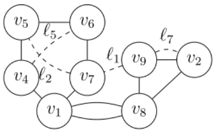
7 1.4 Publications and Manuscripts v1 v8 v9 v2 v7 v4 v6 v5 ¸1 ¸2 ¸5 ¸7
Figure 1.2. An instance of the Connectivity Augmentation Problem. The links are
shown by the dashed edges.
adding a proper family of extra constraints to the standard cut LP. Recently, Grandoni et al. [2018] achieved a 1.458 approximation for TAP, which is smaller than the integrality gap of the standard cut LP.
No much progress was done specifically on CacAP until 2020. Here the best-known approximation factor was still 2, and this factor can be achieved with multiple approaches: Frederickson and JáJá [1981]; Goemans et al. [1994]; Jain [2001]; Khuller and Thurimella [1993]. Altogether this implied that the best known approximation factor for CAP is 2, i.e. the same factor that can be achieved with the much more general approach by Jain [2001]. In Byrka et al. [2020] we obtained the first approximation factor below 2 for CacAP by presenting a 1.91-approximation algorithm based on a method different from the recent advances for TAP.
Very recently, Cecchetto et al. [2021] made an amazing breakthrough re-garding the approximability of CAP by achieving a 1.393-approximation. No-tice that this even improves on the TAP approximation algorithm by Grandoni et al. [2018]. Interestingly the authors bridged the gap between TAP and Ca-cAP by presenting techniques that allow for leveraging insights and methods from TAP to approach CAP.
1.4 Publications and Manuscripts
In this dissertation I will describe my results related to survivable network design. This led to the following two publications:
• On the Cycle Augmentation Problem: Hardness and
Approx-imation Algorithms (Gálvez et al. [2021]). Joint work with Waldo
Gálvez, Fabrizio Grandoni and Krzysztof Sornat. Published in Journal
8 1.5 Our results and Outline of the Thesis
• Breaching the 2-Approximation Barrier for Connectivity
Aug-mentation: A Reduction to Steiner Tree (Byrka et al. [2020]). Joint
work with Jaros≥aw Byrka and Fabrizio Grandoni. Published in STOC
2020.
During my Ph.D. I also worked on other problems which are not described in this thesis since they deviate too much from its main topic. In particu-lar, I studied some geometric packing problems, where the general aim is to pack rectangles in a given region. In particular I worked on the Strip Pack-ing problem and one of its variants. This led to the followPack-ing publication and manuscript:
• A Tight 32 + ‘ Approximation Algorithms for ”-skewed Strip Packing Problem. (Gálvez et al. [2020]). Joint work with Waldo
Gàlvez, Fabrizio Grandoni, Arindam Khan, Klaus Jansen and Malin Rau. Published in APPROX/RANDOM 2020.
• On the Demand Strip Packing Problem. Manuscript. Joint work with Waldo Gàlvez, Fabrizio Grandoni, and Kamyar Khodamoradi. Finally, I worked on some problems independently from my research group at IDSIA. This led to the following publication and manuscript:
• On the Triangle Enclosure Problem. (Jabal Ameli et al. [2018]). Joint work with Hamid Zarrabi Zadeh. Published in ICCG 2018.
• Chromatic Number and Dichromatic Polynomial of Digraphs. Manuscript(Akbari et al. [2017]). Joint work with Saeed Akbari, Amir Ghodrati and Morteza Saghafian.
1.5 Our results and Outline of the Thesis
In Chapter 2 we provide the basic notation, definitions and basic results. We focused on CacAP, with the aim of improving the approximation factor for this problem (hence for CAP). As a first step in this direction, we stud-ied the Cycle Augmentation problem (CycAP), i.e. the special case of CacAP where the input cactus consists of a single cycle. We remark that this spe-cial case remains non-trivial. In Chapter 3 we describe our results on CycAP, namely presenting two approximation algorithms for the problem with approx-imation factor below 2, showing that this problem is APX-hard and presenting
9 1.5 Our results and Outline of the Thesis
a new LP-formulation for this problem with a better integrality gap than the previously known LP-formulations.
Our second, and most relevant result, is an improved 1.91 approximation for CacAP using a reduction to the Steiner Tree problem. This also implies the same approximation factor for CAP based on the mentioned reduction and the known results for TAP. We explain this result in Chapter 4.
Finally, in the Chapter 5 we conclude this thesis and discuss some open problems and future research directions. We defer to the Appendix some rather technical proofs and complementary results.
Chapter 2
Preliminaries
2.1 Edge-connectivity
In this section we discuss basic definitions and useful results related to edge-connectivity. Recall that a graph G = (V, E) is k-connected if by removing any subset of size less than k from E, the graph remains connected.
A subset EÕ ™ E of G is a called an edge-cut (or simply cut) if H =
(V, E \ EÕ) is disconnected. Finding a cut with minimum size (or shortly a
min-cut) is a well-studied classic problem. The size of the min-cut in a graph
Gis known as the edge-connectivity of the graph G and is denoted by ŸÕ(G) (i.e ŸÕ(G) is the smallest k such that G is k-connected). In many applications such
as network systems having edge-connectivity up to some degree is a measure of the reliability and resilience of the system.
Observation 6. Let G be a graph. Then G is k-edge-connected if and only if
the size of the min-cut of G is at least k.
Note that one can disconnect a graph G by removing all the edges incident to a node v of G, therefore:
Observation 7. Let G be a k-connected graph, then for every vertex v of G,
degG(v) Ø k.
Observation 7 suggest that for a graph G the minimum degree of the vertices of G (”(G)) is a lower bound on the edge-connectivity of G. This basic lower bound is very useful to lower bound the optimal solution in several connectivity related optimization problems. In fact, in Chapters 3 and 4 we are using this fact to analyse our approximation factor.
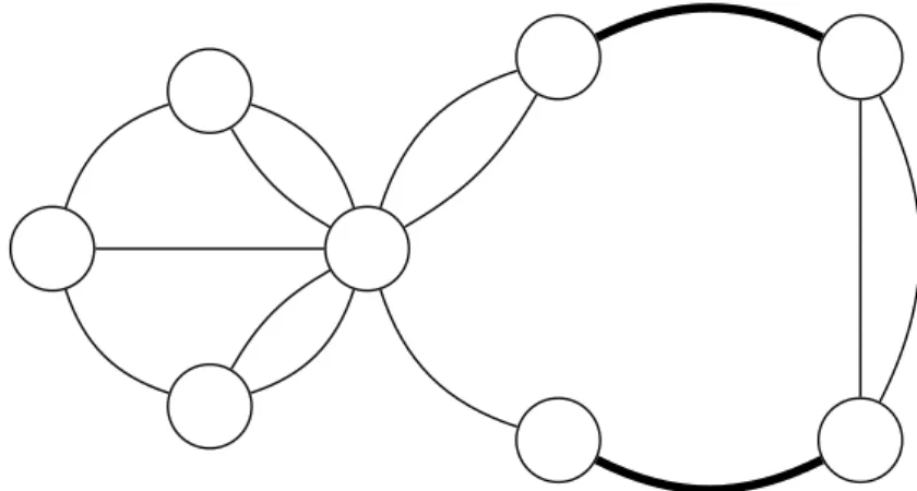
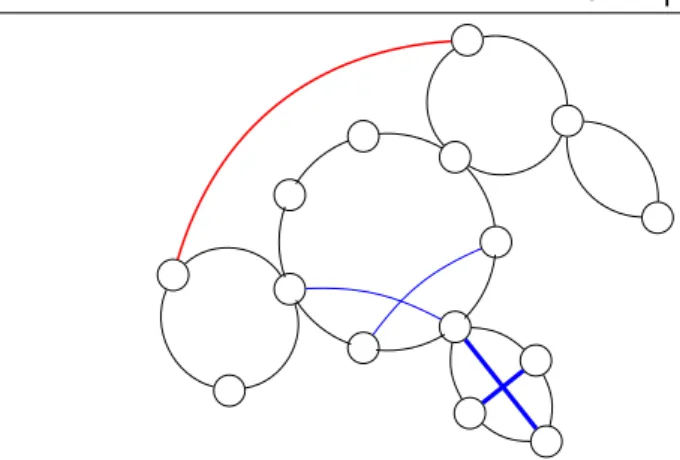
12 2.2 From CAP to TAP and CacAP
Figure 2.1. A graph G with edge-connectivity of 2. The bold black edges indicate
an edge-cut of size 2.
An edge-cut EÕ is called a s ≠ t cut if there is no path from u to v in
H = (V, E \ EÕ).
Many polynomial time algorithm exist for finding the min-cut of a graph and hence checking if a graph is k-edge connected can be done in polynomial time (see Cormen et al. [2009]).
Edge-connectivity is related to the number of edge-disjoint paths among pairs of vertices:
Theorem 8 (Menger’s Theorem). The size of the minimum s≠t cut in a graph
G= (V, E) is k if and only if the maximum number of edge-disjoint paths from u to v is k.
Corollary 9. A graph G = (V, E) is k-connected if and only if for every pair
{u, v} ™ V , there exist k edge-disjoint paths from u to v.
Note that similar definitions and theorems also hold for node-connectivity. To have a more detailed understanding in the subject of connectivity we refer the reader to Bondy and Murty [2008].
2.2 From CAP to TAP and CacAP
In this section we describe an insightful result regarding connectivity augmen-tation proposed by Dinitz et al. [1976], that influenced all the later works in this area.
13 2.2 From CAP to TAP and CacAP
In this section we sketch the ideas leading to this result. Consider an instance of CAP with input a k-connected graph G and a set L of links. Now consider the connected components formed by removing the min-cuts. Dinitz et al. [1976] showed that these components form a laminar family if k is odd. Furthermore, they showed that the minimum edge cuts of a graph G can be represented in polynomial time as the 2-edge-cuts of a graph GÕ such that
ŸÕ(G) = 2. This resulted in the following important theorem:
Theorem 10 (Dinitz et al. [1976]). Any instance of the Connectivity
Augmen-tation can be reduced in polynomial time to the case that k = 1 for odd k and to k = 2 for even k.
Dinitz et al. showed that this is an S-reduction and this means that in terms of approximability we can restrict our attention only to the case that
k = 1 or 2.
For the case that k = 1, if the input graph G contains a cycle one can reduce the size of the input G by contracting this cycle into a single node. By running this process repeatedly, the graph G becomes a tree. Hence:
Proposition 11. There is a S-reduction from Connectivity Augmentation with
k = 1 to TAP
When k = 2, Dinitz et al. [1976] showed that one can contract a pair {u, v} of vertices of G, such that there are at least three edge-disjoint paths from u to v (also known as 3-edge-connected pair). Note that this operation does not violate 2-edge-connectivity. After exhausting this process using the following lemma we show that the ultimate graph Gú is a cactus.
Lemma 12. Let G be a 2-connected graph. Assume that for any pair of vertices
of G such as {u, v}, there are at most two edge-disjoint paths from u to v. Then G is a cactus.
Proof. Assume on the contrary that this is not true. Then, since G is
2-connected, any edge e œ E(G) belongs to at least one cycle of G and since G is not a cactus there exists and edge e1 œ E(G) such that e1 = {v1, v2} belongs
to more than one cycle. Let C1 and C2 be two distinct cycles of G that contain
e1. Now let C1 = v1v2...vkvk+1 (vk+1 = v1). Set i > 1, as the smallest index such that vivi+1, is not an edge of C2. Let vj (i < j Æ k + 1) be the node that has the shortest path, P , to vi in C2. Note that since C2 is a cycle that
contains e1 such a node must exist. Now P , vivi+1...vj and vj...vkv1v2....vi are three edge-disjoint paths from vi to vj which is a contradiction.
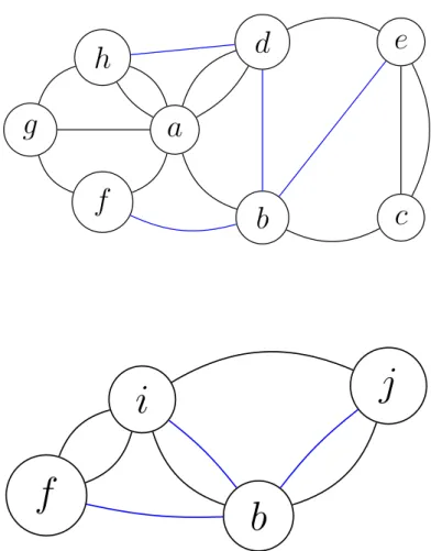
14 2.2 From CAP to TAP and CacAP
a
b
c
d
e
f
g
h
i
b
j
f
Figure 2.2. Top: An instance I of CAP with k = 2. Bottom: An instance J
of CacAP obtained from I by contracting 3-edge-connected pairs of nodes. The node i is obtained from contracting g, h, a and d into one node and the node j is obtained from contracting c and e.
15 2.3 Related Problems
Proposition 13. There is a S-reduction from Connectivity Augmentation with
k = 2 to CacAP.
The following lemma shows that CacAP is at least as hard to approximate as TAP:
Lemma 14. There exists an strict reduction from TAP to CacAP.
Proof. Consider an instance I of TAP with input tree T = (V, E) and the set L of links. From this we obtain an instance of CacAP. Let C = (V, EÕ) be the
cactus formed by duplicating the edges of T . Now assume J is the instance of CacAP formed by input cactus C and links L.
A critical observation is that the set of edge-cuts of size 2 in C are precisely the pair of edges {e, eÕ} such that eÕ is the duplicate of e. This suggests that
the components formed by removing the minimum edge-cuts in I and J are exactly the same. Therefore any subset LÕ ™ L is a feasible solution for I if
and only if it is a feasible solution for J.
Using lemma 14 one can obtain the following statement which is a refined version of theorem 10:
Corollary 15. There exists an S-reduction from CAP to CacAP.
2.3 Related Problems
In this section we discuss some related Survivable Network Design problems. A very closely related problem to CAP is the minimum spanning k-edge-connected
subgraph (k-ECSS), which we proceed to define:
Definition 16 (Minimum Spanning K-edge-connected Subgraph Problem).
In the Minimum Spanning K-edge-connected Subgraph Problem, given a graph G and an integer k, the goal is to find a k-edge-connected spanning subgraph of G with minimum number of edges.
Note that when k = 1, the k-ECSS problem is equivalent to finding a spanning tree of the input graph G, hence we can solve this problem efficiently. However, this problem is NP-hard already for k = 2. Indeed, in this case the size of the optimal solution for this problem is equal to the number |V (G)| of nodes if and only G has a Hamiltonian cycle. Moreover, it has been shown that this problem does not admit PTAS for any k > 1 even for subcubic1 graphs.
16 2.3 Related Problems
In terms of approximability 2-ECSS is a very well-studied problem. The first result beating the factor 2 is the 3
2-approximation algorithm by Khuller and
Vishkin [1994]. Cheriyan et al. [2001] improved the factor to 17
12. A relatively
recent paper by Sebö and Vygen [2014] provides a 4
3-approximation algorithm
given by using more elegant ear decompositions. Hunkenschröder et al. [2019] obtain the same approximation factor by via a drastically different approach.
Surprisingly as k grows, it is easier to approximate k-ECSS. In this line of research, an important result is by Gabow et al. [2009], in which using a LP rounding technique, authors achieved an approximation algorithm of factor 1 + 2
k for even k and 1 +
3
k for odd k.
A very interesting generalization of TAP and 2-ECSS is the Forest
Aug-mentation Problem (FAP):
Definition 17 (Forest Augmentation Problem). In the Forest Augmentation
Problem, as an input we are given a forest G = (V, E) and a set of links L and the goal is to find a subset LÕ of L with minimum size such that G = (V, E fiLÕ)
is 2-connected.
Note that in a point of view, 2-ECSS and TAP are the extreme cases of FAP, where in one problem the forest G contains no edge and in the other problem G has the maximum possible number of edges (i.e., it is a spanning tree). To the best of our knowledge, there is no approximation algorithm with approximation guarantee better than 2 for FAP. Another studied variant of FAP, is the Matching Augmentation problem (MAP), in which the forest G is simply a matching. MAP was first introduced in Cheriyan, Dippel, Grandoni, Khan and Narayan [2020], who present a 7
4-approximation for this problem.
The approximation factor was later improved to 5
3 by Cheriyan, Cummings,
Dippel and Zhu [2020].
All the mentioned problems are special cases of the following very general survivable network design problem.
Definition 18. (The Steiner Network Problem) In the Steiner Network
prob-lem as an input we are given:
• A graph G = (V, E) with non-negative weights on the edges. • And for each pair of vertices {u, v} ™ V , a number fu,v.
The goal is to find a subgraph H of G with minimum total weight such that for every pair of vertices {u, v} ™ V , there are fu,v edge-disjoint paths from u to v
17 2.3 Related Problems
For this problem Jain [2001] achieved a 2-approximation using an interesting iterative LP rounding technique. It is not hard to show that approximating Steiner Network is at least as hard as approximating CAP and k-ECSS.
Lemma 19. There exists an strict reduction from CAP to the Steiner Network
problem.
Proof. Consider an instance I of the Connectivity Augmentation with the
k-connected graph G = (V, E) and the set of links L. We transform this to an instance J of the Steiner Network in the following manner. We set GÕ =
(V, E fiL) and we assign weight zero and one to E and L, respectively. For each pair of vertices of G also set the values of fu,v to k + 1. Now using Theorem 8, any feasible solution of size l for I is a feasible solution of cost l for J and vice-versa.
Lemma 20. There exists an strict reduction from k-ECSS to the Steiner
Net-work problem.
Proof. Consider an instance I of k-ECSS with the input graph G and k. From
this we obtain an instance J of the Steiner network design in the following manner. We set GÕ = (V, E) and we assign weight one to E. For each pair of
vertices of G also set the values of fu,v to k. Now using Theorem 8, a subset of edges EÕ is a feasible solution for I if and only if EÕ is a feasible solution for
J.
A simple variant of CAP is when there is a link for every pair of vertices. Unlike the previously mentioned problems, there is a polynomial-time exact algorithm for this problem (Watanabe and Nakamura [1987]).
One can consider also a weighted version of CAP, the Weighted Connectivity
Augmentation problem (WCAP), where links have a positive weight and our
goal is to minimize the total weight of selected links LÕ. The same reduction
as mentioned before also works in the weighted case. In particular, one can re-duce WCAP to weighted version WTAP of TAP for odd k, and to the weighted version WCacAP of CacAP for even k. The best-known approximation factor even for WTAP (hence for WCAP) is 2. This factor was first established by Frederickson and JáJá [1981]. Their algorithm was later simplified by Khuller and Thurimella [1993]. A 2-approximation can also be achieved by various other techniques developed later on, including a primal-dual approach (Goe-mans et al. [1994]) and iterative rounding (Jain [2001]). Improvements on the factor 2 have only been obtained for restricted cases, including bounded diam-eter trees (Cohen and Nutov [2011]) and bounded weights (Adjiashvili [2017];
18 2.3 Related Problems
Fiorini et al. [2018]; Grandoni et al. [2018]; Nutov [2017]). Very recently Traub and Zenklusen [2021] published a paper on arXiv in which they provide a (1 + ln 2 + ‘)-approximation for WTAP.
Another related problem is the node-connectivity augmentation in which given a k-node-connected graph G and a set of links L, the goal is to find a minimum size subset LÕ of L such that G = (V, E fi LÕ) is (k +
1)-node-connected. One can observe that increasing connectivity by one already poses significant challenges and in general the node-connectivity versions of these problems seem to be more difficult than their edge-connectivity counterparts.
The best-studied version is when k = 1, known as Block-Tree Augmentation:
Definition 21 (Block-Tree Augmentation Problem). Given a tree T = (V, E)
and a set of links L on V , the goal is to find a minimum size subset LÕ of L
such that G = (V, E fi LÕ) is 2-node-connected.
Frederickson and JáJá [1981] and Khuller and Thurimella [1993] achieved a 2-approximation for Block-Tree Augmentation. However, unlike the edge-connectivity counterpart (TAP), an approximation algorithm with ratio better than 2 was achieved only very recently by Nutov [2020]. Nutov exploits our 1.91-approximation algorithm for CacAP (Byrka et al. [2020]) as a black box.
Chapter 3
The Cycle Augmentation Problem
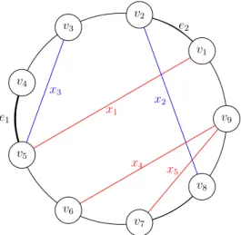
Our first attempt to attack the 2-approximation barrier for the Cactus Aug-mentation problem (CacAP) was to investigate some interesting special cases. In particular, we introduced the Cycle Augmentation problem (CycAP), which is the special case of CacAP where the input cactus is a cycle. Figure 3.1 illustrates an instance of CycAP.
The best known approximation factor for this special case was still 2, like for the general case, and CycAP was even not know to be NP-hard. We also consider the natural weighted version WCycAP of CycAP. We obtained the following main results:
• We present a fast and simple 5
3-approximation for CycAP.
• We present a slower (still polynomial-time) (3
2 + ‘)-approximation for
CycAP.
• We show that CycAP is APX-Hard.
• We show that WCycAP is as hard to approximate as WCacAP.
• We introduce a new LP-formulation for CycAP with integrality gap of (3
2 + ‘).
Our first result is obtained via a greedy algorithm. The second result is based on a procedure to solve the problem exactly and efficiently when there are no long links. More precisely, we show that CycAP is FPT on the maximum distance of the endpoints of the links. These first two results are described in Section 3.2.
Our third result (see Section 3.3) shows that CycAP does not admit a PTAS. We remark that prior to our work this special case was not even known
20
Figure 3.1. An instance of CycAP. The blue edges are the input links. The bold
links form an optimal solution.
to be NP-hard. NP-hardness was not obvious at all. In particular, if we replace the cycle with a path the problem can be solved exactly in polynomial time.
Our fourth result (see Section 3.4) shows that in the weighted case there is no substantial difference between WCycAP and WCacAP. Hence unfortunately focusing on the cycle case cannot help much as a first step towards addressing the general case. On the positive side, researchers might focus on the cycle case which is easier to state.
The recent literature on TAP approximation (Adjiashvili [2017]; Fiorini et al. [2018]; Grandoni et al. [2018]) shows that finding strong LP relaxations for the problem can be very helpful to design improved approximation algorithms. In the same spirit, we tried to address the problem of finding LP relaxations for CycAP with small integrality gap. For both TAP and CacAP (hence CycAP) one can define a natural and simple standard cut LP (more details later).
While for TAP it was recently shown that the standard cut LP has inte-grality gap smaller than 2 (Nutov [2017]), interestingly for CycAP (hence for CacAP) the standard cut LP has integrality gap 2. As the final result we present a stronger LP that, for any Á > 0, has integrality gap at most 3
2 + Á
(hence matching the approximation ratio of our algorithm). In our opinion this could be useful for future work on CacAP approximation.
21 3.1 Definitions and Notations
3.1 Definitions and Notations
For a set X and element y, we use the shortcut X \y for X \{y}, and similarly for other set operations.
Given a graph G = (V, E), we let V (G) = V and E(G) = E. Recall that in WCacAP we are given a cactus G = (V, E), a set of links L ™ 1V
2
2
and a non-negative weight function c : L æ RØ0. The task is to compute a
subset of links A ™ L such that the graph (V, E fi A) is 3-connected while minimizing c(A) := q¸œAc(¸). The special case where G is a cycle is called
WCycAP, and the unweighted versions of the above problems are called CacAP and CycAP respectively. By n we will denote the number of nodes of the considered instance of the problem.
Notice that, given an instance (G, L) of CacAP, we can check in polynomial time if the graph (V (G), E(G) fi L) is 3-connected by exhaustively checking if the removal of any pair of elements from E(G) fi L disconnects the graph. Hence we will assume along this work that the instance always admits a feasible solution.
Observation 22. The 2-edge cuts of a cactus G are identified by pairs S =
{e, eÕ} of distinct edges belonging to the same cycle, and consist of the node sets
(U, V \U) of the two connected components obtained by removing S from G. A
necessary and sufficient condition for a subset of links A to be a feasible solution for WCacAP is that, for any such cut S, there is at least one ¸ =< u, v >œ A that u œ U and v œ (V \ U). (in which case ¸ satisfies the {e, eÕ}-cut).
Note that in the case of CycAP, Observation 22 implies that any feasible solution must be an edge cover as 2-edge cuts defined by neighboring edges of the cycle must be satisfied. Given a 2-edge cut S = {e, eÕ}, let L
S be the subset of links satisfying S. The standard cut LP for CycAP is as follows:
min ÿ ¸œL x¸ (standard cut LP) s.t. ÿ ¸œLS x¸ Ø 1 ’S : S is a 2-edge cut 0 Æ x¸ Æ 1 ’¸ œ L
Now we proceed to define a standard building block for our algorithms, the
contraction of a link.
Definition 23. Contracting a subset of nodes W consists of the following
op-erations: (i) remove the nodes in W and all edges/links incident to them; (ii) add a new node w and, for each original edge/link of type (y, x), x œ W, y /œ W,
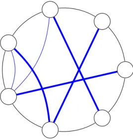
22 3.1 Definitions and Notations v1 v2 v3 v4 v5 v6 v7 v8 v9 v1 v2 v3 v4 v5 v6 v7 v8 v9 x1 x2 x3 x4 x5 e1 e2
Figure 3.2. Depiction of the Standard cut LP. The blue links are the set of all
the links that satisfy the cut {e1, e2}. Therefore this corresponds to the following
constraint: x2+ x3 Ø 1.
add the edge/link (y, w) (of the same weight for the case of links). Note that we do not create loops this way but may introduce parallel links. We say that
(y, w) is the image of (y, x) and (y, x) is the preimage of (y, w).
We will sometimes slightly abuse notation and use the same label to denote a link and its image: the meaning will be clear from the context.
For a link ¸ = (u, v), we define a sequence w0, . . . , wq of boundary nodes
B(¸) as follows. Consider a simple path from u to v in the cactus, and let C1, C2, . . . , Cq be the ordered sequence of cycles visited by this path (possibly
q = 1). Note that a path visits a cycle iff it includes an edge from the cycle.
We define wi, i = 1, . . . , q ≠ 1 as the unique common node between Ci and
Ci+1, and set w0 = u and wq = v.
Definition 24. Contracting a link ¸ is the operation of contracting its boundary
nodes B(¸). We denote by G|¸ the graph obtained by this operation. Contracting a set of links A is the operation of contracting any ¸ œ A, and then continue recursively on G|¸ and on the image of A \ ¸ until A becomes empty.
Note that contracting a link in a cactus yields again a cactus. We will extensively use the following standard fact.
Lemma 25. Let (G, L) be a CacAP instance, A ™ L, and ¸ œ A. Then A
is a feasible solution for (G, L) iff the image of A \ ¸ is a feasible solution for
23 3.1 Definitions and Notations
We require some further notation before proving the lemma. The internal
projections S(¸) of ¸ are the links (wi, wi+1), i = 0, . . . , q ≠ 1. In terms of feasibility, ¸ and S(¸) are equivalent as the following proposition states.
Proposition 26. Let (G, L) be a CacAP instance and ¸ œ L. Then ¸ satisfies
precisely the same 2-edge cuts as S(¸).
Proof. Let B(¸) = (w0, . . . , wq) and C1, . . . , Cq be the corresponding sequence of cycles visited by a simple path between the endpoints of ¸. Notice that pairs (wi, wi+1), i = 0, . . . , q ≠ 1, subdivide each Ci into two paths next denoted as
CÕ
i and CiÕÕ. Trivially ¸ satisfies only cuts belonging to the cycles C1, . . . , Cq, and the same holds for S(¸). Consider any pair (e1, e2) belonging to some Ci.
Link ¸ satisfies the corresponding cut if and only if precisely one such edge ej belongs to CÕ
i. The same holds for (wi, wi+1), hence for S(¸).
In order to prove Lemma 25, let us first consider the simpler case where G is a cycle.
Lemma 27. Let (G = (V, E), L) be a CycAP instance, A ™ L, and ¸ =
(u, v) œ A. Then A is a feasible solution for (G, L) iff the image of A \ ¸ is a
feasible solution for the CacAP instance (G|¸, L \ ¸).
Proof. Let C1 and C2 be the two cycles in G|¸, with common node w.
Suppose first that the image of A \ ¸ is a feasible solution for (G|¸, L \ ¸). Consider a pair of edges {e1, e2} belonging to a common cycle Ci, and the
corresponding cut (SÕ, SÕÕ) in G|¸ with w œ SÕÕ. There must be a link ¸Õ œ A \ ¸
satisfying this cut in G|¸. The preimage of ¸Õ has one endpoint in SÕ and the
other in V \ SÕ = (SÕÕ\ {w}) fi {u, v}, hence it satisfies the {e1, e2}-cut in G.
The remaining pairs of edges {e1, e2} of G satisfy e1 œ C1 and e2 œ C2, modulo
symmetries. Those cuts are satisfied by ¸ in G.
Suppose now that A is feasible for (G, L). Consider a pair of edges {e1, e2}
belonging to a common cycle Ci. Let (SÕ, SÕÕ) be the corresponding cut in G|¸
with w œ SÕÕ. Since ¸ does not satisfy that cut in G, this means that there is
some other link ¸Õ œ A \ ¸ satisfying it. The image of ¸Õ has one endpoint in SÕ
and the other in SÕÕ, hence it satisfies the {e1, e2}-cut.
Now we can proceed with the proof of Lemma 25.
Proof of Lemma 25. By Proposition 26, we obtain an equivalent statement of
the lemma by replacing A with the set S(A) of the internal projections of links in A and replacing ¸ with its internal projection S(¸).
24 3.2 Approximation algorithms
Figure 3.3. The graph G is introduced by the black edges, the internal links are
shown by the blue edges and the red edge is an external link. The bold blue edges are a pair of crossing internal links.
Let B(¸) = (w0, . . . , wq) and C1, . . . , Cq be the corresponding sequence of cycles visited by a simple path between the endpoints of ¸. Consider any cycle
C not in the above list. Then trivially any pair of edges in C is covered by
links in S(A) \ S(¸). Therefore it is sufficient to consider pairs of edges e1, e2
belonging to the same cycle Ci. Let ¸i = (wi, wi+1) be the internal projection of ¸ with both endpoints in Ci, and define similarly Si(A) w.r.t. S(A). Then it is sufficient to show that Si(A) is a feasible solution for the CycAP instance induced by Ci if and only if Si(A) \ ¸i is a feasible solution for the CycAP instance induced by Ci|¸i, which follows from Lemma 27.
3.2 Approximation algorithms
In this section, we present our approximation algorithms for CycAP. We start with a simple 5
3-approximation to show our main intuition and illustrate the
main ideas. Then we present a slightly more complex 13 2 + ‘
2
-approximation. Both algorithms are based on greedy choices of links. The approach we will follow in both cases is as follows: in the first phase, we iteratively add a prop-erly chosen subset of a few links to the solution under construction, and then contract them. Notice that, after the first contraction, the cycle structure may be lost and we obtain a CacAP instance instead. These choices are designed so that, at the end of the first phase, the remaining CacAP instance can be solved efficiently, which is done in a second phase with an ad-hoc algorithm. We remark that the running times of the presented algorithms are not analyzed in detail, and indeed such a task may require to devise carefully crafted data structures.
25 3.2 Approximation algorithms
We next describe a simple greedy algorithm that provides a5
3-approximation
for CycAP. We need the following definitions.
Definition 28. A link ¸ = (u, v) of a CacAP instance is internal if both its
endpoints belong to a common cycle, and external otherwise.
Definition 29. Given a CacAP instance, a pair of internal links {(u1, v1), (u2, v2)}
of a cycle C is crossing if they are node disjoint and deleting u2 and v2
dis-connects u1 from v1 in C.
In the first stage of the algorithm we only add external links plus crossing pairs of links. More in detail, the algorithm has two main stages. The first stage consists of a set of rounds, where in each round we first check if there exists an external link ¸, in which case we add it to our solution, contract it and proceed to the next round. Otherwise, if there exists a pair of (internal) crossing links
¸Õ and ¸ÕÕ, we add them to our solution, contract them and proceed to the
next round. If none of the two cases above applies, we are left with a CacAP instance without any external link or crossing pairs of links which we address in the second stage of the algorithm. We refer to this algorithm as crossing-first. As the following lemma states, in the second stage we can efficiently compute the optimal solution.
Lemma 30. Consider an instance (G = (V, E), L) of CacAP. If there are no
external links and no crossing pairs of links, then every minimal solution has size exactly |V | ≠ 1 and induces a spanning tree over V .
Proof. We prove the first part of the claim by induction on n = |V |. The base
case n = 2 is trivial since in this case the instance is just a cycle consisting of two parallel edges and any link must be incident to the two nodes of G (hence defining a feasible solution). For the inductive case, assume the claim is true up to instances having n ≠ 1 nodes, and consider an instance of the problem defined by a cactus G having n nodes with optimal solution OPT. If G is not a cycle of length n, then it is defined by a set of cycles of length at most n ≠ 1 where every link is internal, so we can apply the inductive hypothesis to each cycle independently. If G is a cycle of n nodes, then let ¸ = (u, v) œ OPT. Contracting ¸ leads to a CacAP instance on two cycles C1 and C2 sharing
a common node w, with |V (C1)| + |V (C2)| = n. Let OPTÕ be the optimal
solution for the new instance. By Lemma 25, |OPT| = |OPTÕ| + 1. Observe
that any remaining link ¸Õ must have both endpoints in the same Ci (otherwise
¸ and ¸Õ would be crossing). Thus by the inductive hypothesis the optimum
26 3.2 Approximation algorithms
that |OPTÕ| = |V (C1)| ≠ 1 + |V (C2)| ≠ 1 = n ≠ 2. Hence |OPT| = n ≠ 1 as
desired.
For the second part of the claim, it is sufficient to show that a minimal solution does not induce a cycle. By contradiction, consider a minimal solution containing a simple cycle LÕ, and consider now a solution where we remove
precisely one arbitrary link ¸ = (u, v) from LÕ. Consider any pair of edges e1, e2
belonging to the same cycle such that ¸ satisfies the {e1, e2}-cut. Since LÕ \ ¸
induces a simple u-v path, then some ¸Õ œ LÕ \ ¸ must satisfy the cut. Thus
LÕ\ ¸ is a feasible solution, contradicting the minimality of LÕ.
By showing that the number of links in the second stage is a lower bound on the size of the optimal solution we obtained the following result:
Theorem 31. The crossing-first algorithm is a 5
3-approximation for CycAP.
Proof. Let OPT be the optimal solution and APX the computed solution. Let
also nÕÕ be the number of nodes remaining at the end of the first stage, and
APXÕ (resp. APXÕÕ) be the set of links added to the solution during the first
(resp. second) stage. Since contracting an external link decreases the number of nodes by at least 2 and contracting any pair of crossing links decreases the number of nodes by at least 3, we have that |APXÕ| Æ 2
3(n ≠ nÕÕ).
By Lemma 30, |APXÕÕ| = nÕÕ≠ 1, and hence |APX| Æ 2
3(n ≠ nÕÕ) + nÕÕ≠ 1 = 2n+nÕÕ≠3
3 . On the other hand, since any feasible solution must be an edge cover,
we have that |OPT| Ø n/2. Observe also that |OPT| Ø nÕÕ≠ 1 since by Lemma
25 contracting links cannot increase the cost of the optimum solution. Thus |OPT| Ø max{n/2, nÕÕ ≠ 1}. We can conclude that |APX|
|OPT| Æ
(2n+nÕÕ≠3)/3
max{n/2,nÕÕ≠1} Æ 53,
being nÕÕ≠ 1 = n/2 the worst case.
Finally we designed an input showing that the approximation ratio of crossing-first is no better that 5
3 (see Figure 3.4), which shows that our analysis
in the proof of theorem 31 was tight.
Lemma 32. The approximation ratio of the crossing-first algorithm is not
better than 5 3.
Proof. Consider the following construction: for each k Ø 2 consider an instance
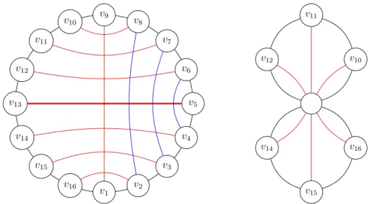
(Gk, Lk) of CycAP defined by a cycle of n = 6k nodes (assume that the cycle is
defined by the order of the nodes v1, v2, . . . , v6k) and the following set of links
(see Figure 3.4 (Left)): • (v1, vn
27 3.2 Approximation algorithms v1 v2 v3 v4 v5 v6 v7 v8 v9 v10 v11 v12 v1 v2 v3 v4 v5 v6 v7 v8 v9 v10 v11 v12 v1 v5 v6 v7 v8 v9 v10 v11 v12
Figure 3.4. Left: Instance (G2, L2) from the lower bound construction in
Lemma 32. Red links define an optimal solution. Right: If the algorithm in the first phase picks and contracts the crossing links {(v1, v3), (v2, v4)}, this is the
obtained CacAP instance.
• For each i = 1, . . . ,n
2 ≠ 1, (vi+1, vn+1≠i) œ Lk; • For each i = 1, . . . ,n
6, (v3(i≠1)+1, v3(i≠1)+3) œ Lkand (v3(i≠1)+2, v3(i≠1)+4) œ
Lk;
Notice that the first and second set of links define a feasible solution of size n
2, hence being optimal: if we remove any two edges of the cycle, then
we are either satisfying the corresponding cut via (v1, vn
2+1), or one side of the
partition is contained in either {v2, . . . , vn
2} or in {vn2+2, . . . , vn} but the links
selected form a matching between those sets.
We will now prove that there exists a sequence of choices performed by our algorithm that outputs a solution of size 5n
6 ≠ 1, which implies that the
approximation ratio is at least 5
3 ≠ 2n and this value approaches
5
3 as k goes to
infinity. Notice first that the pair of links {(v1, v3), (v2, v4)} ™ Lk is crossing,
and hence the algorithm can include them in the solution in the first round (and finish the round). Furthermore, after these links are contracted no link becomes external as the new cactus instance consists of a cycle of length n ≠3, and also the links with endpoints vn, vn≠1 and vn≠2 are not part of any pair of
crossing links (see Figure 3.4 (Right)). If we now iteratively pick all the pairs of crossing links {(v3(i≠1)+1, v3(i≠1)+3), (v3(i≠1)+2, v3(i≠1)+4)} ™ Lk, i = 2, . . . ,n6,
after n
6 rounds we end up with a cycle of length n2 without crossing links, and
the algorithm must now take the remaining n
2≠1 links to complete the solution.
Thus, the size of the computed solution is 2 · n
28 3.2 Approximation algorithms
claim.
Now we describe our more advanced (3
2+‘)-approximation algorithm. Here
we introduce a new classification of the links, namely a classification by size.
Definition 33. The length of an internal link (u, v) is the length of the
short-est path between u and v in the corresponding cycle. For a given parameter
0 < ‘ < 1, an internal link is called long if its length is at least 1
Á, and short
otherwise.
Our algorithm consists of the following two main phases. In the first phase, we iteratively check if there exists a long (internal) link ¸. Otherwise, we check if there exists an external link ¸. In both cases, we add ¸ to the solution under construction and contract it. Observe that contracting links does not create new long links, hence we will first select a set Llong of long links, and then a
set Lext of external links.
After exhausting the previous choices, we move to the second phase. Here we are left with an instance where all links are short and internal. This allows us to solve independently the sub-instance induced by each cycle. We refer to this algorithm as long-first. This second stage can be solved efficiently, due to the lack of long links, by means of the following lemma1.
Lemma 34. Given a CycAP instance, there exists an algorithm based on
dy-namic programming that returns the optimal solution in time poly(n) · 2O(h2max),
where hmax is the maximum length among the links.
Let Lshort be the collection of edges obtained in the second stage. The final
solution is LlongfiLextfiLshort. The intuition is that |Llong| is very small compared
to the size of the optimal solution, external edges are greedily good choices and
Lshort is an exactly optimal solution for the final stage and is a lower-bound for
the size of the optimal solution.
Theorem 35. The long-first algorithm is a (3
2 + Á)-approximation algorithm
for CycAP.
Proof. The running time of the algorithm is upper-bounded by poly(n)2O(1/Á2). Consider next the approximation factor. Note first that |Llong| Æ Án. Indeed,
contracting a long link always increases the number of cycles in the cactus by one without decreasing the number of edges, and all these cycles always have
29 3.2 Approximation algorithms
size at least 1/Á, so there are at most Án of them. Similarly to Theorem 31, we have that |OPT| Ø |Lshort| and |OPT| Ø n2.
If |Llong|+|Lext|+|Lshort| Æ (3+2Á)n4 then we already have a
13
2 + Á
2
-approximation as |OPT| Ø n
2. Otherwise, since the contraction of each external link reduces
the number of nodes by at least 2 and the contraction of any other link reduces the number of nodes by at least 1, we have that |Llong|+2|Lext|+|Lshort| Æ n. So
|Lext| Æ n ≠(3+2Á)n4 = (1≠2Á)n4 and hence |Lext| + |Llong| Æ n+2Án4 Æ
11
2 + Á
2
|OPT|. Since |OPT| Ø |Lshort|, we have that in this case the size of the solution is also
at most (3
2 + Á)|OPT|, concluding the proof.
Remark 36. By replacing Á with 1/Ôlog n in the above construction, we can
obtain a slightly improved approximation factor of 3/2 + o(1) which still runs in polynomial time.
It remains to prove Lemma 34. To do this, we need some more notations. Given a link ¸ = (u, v), we say that the edges of the shortest path between u and v in the cycle are covered by ¸ (in case of multiple shortest paths we choose the one going from u to v in counter-clockwise order along the cycle). Given an edge e of the cycle, we define the cut-neighborhood of e, namely N (e), as the 2hmax≠ 1 edges that are closest to e, e included. We also define NL(e) as
the set of links in L covering at least one edge from N (e).
Notice that in any feasible solution to a CycAP instance, at most one edge of the cycle is not covered: if it is not the case, then the cut defined by two uncovered edges is not satisfied as any link satisfying the cut would cover one of these two edges. We can use this observation to characterize the feasibility of a solution in terms of the cut-neighborhoods.
Lemma 37. Consider a CycAP instance and let A be a set of links such that
every edge of the cycle is covered by some link in A. A is feasible iff for each edge e, all the {e, eÕ}-cuts, where eÕ œ N (e), are satisfied.
Proof. If A is feasible then the required properties are clearly satisfied since
every cut is satisfied. On the other hand, suppose that A satisfies that every edge is covered by some link in A and the {e, eÕ}-cuts are satisfied for every
edge e and eÕ œ N (e). Consider a pair of edges {e, eÕ} such that eÕ œ N (e)./
By definition of N (e) there is no link in A covering both edges at the same time, and as e is covered by some link, this link satisfies the {e, eÕ}-cut. This
implies that A is feasible as every cut is satisfied.
This lemma is useful as it implies that, given an edge e and a set of links
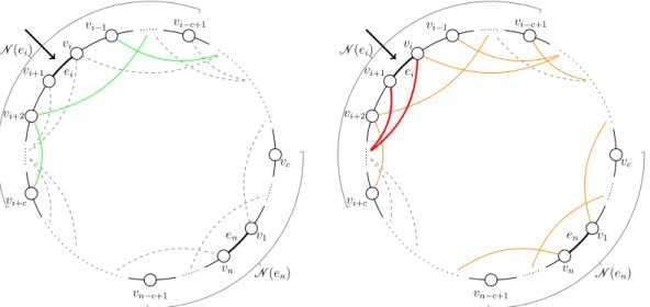
30 3.2 Approximation algorithms vi+1 vi+2 vi vi≠1 vi≠c+1 vi+c vn≠c+1 vn v1 vc N(en) N(ei) ei en vi+1 vi+2 vi vi≠1 vi≠c+1 vi+c vn≠c+1 vn v1 vc N(en) N(ei) ei en
Figure 3.5. Depiction of an iteration of the DP from Lemma 34, where we are
currently at edge ei. Left: Green links correspond to S and at this point we must decide which extra links to add to S in order to satisfy the edges e1, . . . , ei. Right:
This computation is done by looking at a proper previous cell in the table (orange links) which contains S and satisfies e1, . . . , ei≠1, and then add the extra required
links Aú (red links) in order to satisfy ei too.
2O(h2max) just by guessing the subset of links from NL(e) that must be added, which are O(h2
max) only. Now we proceed to present the proof.
Proof of Lemma 34. Let us assume that we deal with instances of CycAP such
that there exists an optimal solution where every edge is covered by some link. If it is not the case, as there may be only one uncovered edge, we can guess this edge and contract it; this leads to an equivalent instance of the problem where we can require that the optimum solution covers all the edges. We say that an edge e is satisfied by a set of links A if it is covered by some link in A and furthermore every {e, eÕ}-cut is satisfied by A. In particular A is a feasible
solution for the problem iff it satisfies all the edges.
We next design a dynamic programming algorithm to compute a minimum cardinality feasible solution. Let us name the nodes v1, v2, ..., vn in counter-clockwise order starting from some arbitrary node v1, and let the edges be
ei = (vi, vi+1) for each i = 1, . . . , n (assuming vn+1 = v1).
For each edge ei and S ™ NL(ei), we define a cell T [i][S] which will corre-spond to a set SÕ of links of smallest cardinality such that for each j œ {1, . . . , i},