HAL Id: inserm-00440689
https://www.hal.inserm.fr/inserm-00440689
Submitted on 11 Dec 2009
HAL is a multi-disciplinary open access
archive for the deposit and dissemination of
sci-entific research documents, whether they are
pub-lished or not. The documents may come from
teaching and research institutions in France or
abroad, or from public or private research centers.
L’archive ouverte pluridisciplinaire HAL, est
destinée au dépôt et à la diffusion de documents
scientifiques de niveau recherche, publiés ou non,
émanant des établissements d’enseignement et de
recherche français ou étrangers, des laboratoires
publics ou privés.
Prior affinity measures on matches for ICP-like
nonlinear registration of free-form surfaces
Benoît Combès, Sylvain Prima
To cite this version:
Benoît Combès, Sylvain Prima. Prior affinity measures on matches for ICP-like nonlinear
registra-tion of free-form surfaces. 6th IEEE Internaregistra-tional Symposium on Biomedical Imaging: From Nano
to Macro (ISBI’2009), Jun 2009, Boston, United States. pp.370-373, �10.1109/ISBI.2009.5193061�.
�inserm-00440689�
PRIOR AFFINITY MEASURES ON MATCHES
FOR ICP-LIKE NONLINEAR REGISTRATION OF FREE-FORM SURFACES
Benoˆıt Comb`es and Sylvain Prima
INSERM, U746, F-35042 Rennes, France
INRIA, VisAGeS Project-Team, F-35042 Rennes, France
University of Rennes I, CNRS, UMR 6074, IRISA, F-35042 Rennes, France
[bcombes,sprima]@irisa.fr, http://www.irisa.fr/visages
ABSTRACT
In this paper, we show that several well-known nonlinear surface reg-istration algorithms can be put in an ICP-like framework, and thus boil down to the successive estimation of point-to-point correspon-dences and of a transformation between the two surfaces. We pro-pose to enrich the ICP-like criterion with additional constraints and show that it is possible to minimise it in the same way as the original formulation, with only minor modifications in the update formulas and the same convergence properties. These constraints help the al-gorithm to converge to a more realistic solution and can be encoded in an affinity term between the points of the surfaces to register. This term is able to encode both a priori knowledge and higher order ge-ometrical information in a unified manner. We illustrate the high added value of this new term on synthetic and real data.
Index Terms— registration, mesh, surface, geometrical invari-ants, optimisation
1. INTRODUCTION
Nonlinear registration is a key tool in medical image analysis for the understanding of anatomy in normal and pathological conditions. It allows the quantitative comparison of structures in different subjects and more generally the fusion of inter-subject data for further statis-tical analysis. Surfaces represented by point clouds or meshes are especially convenient to represent a subject’s anatomy. In particular, they allow to isolate a specific structure or organ from the rest of the body (eg after segmentation from MRI data), and thus to help answer given research questions in a very specific manner. A convenient way to perform nonlinear registration of surfaces is to formulate it as a minimisation problem. Such an approach poses some specific problems, most notably the difficulty 1) to devise a criterion allowing to obtain an adequate solution (eg with a good compromise between regularity and closeness to the data); 2) to minimise such a criterion efficiently (eg with a simple scheme and proofs of convergence).
In this paper, our contributions are twofold. First, we show that several well-known nonlinear registration algorithms can actually be put in an ICP-like framework, that consists in the successive esti-mation of the point-to-point correspondences and the transforesti-mation between the surfaces. Such a framework yields a simple scheme with iterative update formulas for both unknowns that converges to a minimum of a well-grounded criterion (Section 2). Second, we show that it is possible to enrich this criterion with additional constraints, to make it robust using a threshold function, and to minimise it effi-ciently with only minor modifications in the update formulas and the same convergence properties as the original algorithm (Section 3).
These constraints help the algorithm to converge to a more realis-tic solution and can be encoded in an affinity term in the ICP-like general criterion. This affinity term is computed between the points of the two surfaces to register and comes in addition to the proximity term between their spatial coordinates. It is able to encode both a pri-ori knowledge (eg labels of gyri/sulci for cortical registration) (Sec-tion 4.2) and higher order geometrical informa(Sec-tion (eg consistency between the curvatures of points to be matched) (Section 4.1) and thus handles both types of constraints in a unified manner. Finally, we evaluate the added value of this new affinity term on synthetic and real data in Section 5.
2. NON RIGID REGISTRATION AS AN ICP ALGORITHM Numerous algorithms have been proposed for nonlinear registration of 3D surfaces [1]. Many such methods have been largely inspired by the ICP algorithm [2] whose key idea is to consider the regis-tration problem as the interleaved estimation of point-to-point cor-respondences and (rigid-body) transformation between the two sur-faces. In case of the ICP algorithm, this dual view is extremely useful as it allows 1) the formulation of the problem as a minimisation of a well-defined criterion; 2) the optimisation of this criterion via iter-ative and tractable minimisations over the correspondences and the transformation in turn; 3) a proof of convergence towards a (at least local) minimum of this criterion. In fact, these key properties can be kept for nonlinear problems using the same dual view by defining the optimal transformation between two surfacesX and Y as:
˜ T = arg min A,T X xi∈X X yj∈Y Ai,j||yj− T (xi)||2+ αL(T ) (1) +γX i X j
Ai,jlog(Ai,j) with ∀i ,
X
j
Ai,j= 1 and ∀(i, j) , Ai,j ≥ 0
and where:
• T is the transformation best superposing the two sets of points (and that can be rigid, affine, elastic, etc).
• A is a card(X) × card(Y ) matrix. The greater Ai,j, the
more likely the pointxi∈ X to be the correspondent of the
pointyj∈ Y . A can be viewed as a hidden variable of the
registration problem and will be called the match matrix. • L is a regulariser allowing to penalise discontinuities of T
over the space withα > 0 weighing its influence. • γP
i
P
jAi,jlog(Ai,j) is a barrier function allowing to
con-trol the fuzziness ofA (the higher γ, the greater the fuzzi-ness). In practice, this term convexifies the criterion.
The key remark is that this criterion can be minimised by suc-cessive optimisation overA with T fixed and over T with A fixed:
Step 0: Initialise ˜T Step 1: ˜A = arg minAP
xi∈X
P
yi∈YAi,j||yj− ˜T (xi)||
2 +γP
i P
jAi,jlog(Ai,j) with P
jAij= 1 Step 2: ˜T = arg minT
P xi∈X P yi∈Y ˜ Ai,j||yi− T (xi)||2+ αL(T ) Step 3: if ˜T has changed go to Step 1 else exit
This iterative scheme is simple and ensures a monotonical decrease of the criterion (for any transformationT and regulariser L) and thus a convergence towards a (at least) local minimum. Note that the fuzziness ofA and the regularity of T can be adapted throughout the iterations by varying (typically decreasing) the parametersα and γ.
The main challenge is then to define properT and L to make Steps 1 and 2 tractable. Below we list several algorithms fitting in this general ICP-like formulation and detail their choices to do so:
⊲ The original ICP algorithm [2] where T is a rigid-body trans-formation,L is the null function and γ is equal to zero. Step 1 is solved settingAi,jto one if and onlyyjis the closest point ofT (xi)
inY and zero else (typically using a kd-tree). Solving Step 2 then consists in finding the transformation that best superposes the corre-spondences established during Step 1 in the least squares sense.
⊲ The TPS-RPM algorithm [3] where T and L encode smooth-ing Thin Plate Splines andγ is typically set to decrease from infinity (maximal fuzziness) to zero (no fuzziness i.e.A is binary) through-out the iterations. Steps 1 and 2 have a simple closed-form solution but Step 2 requires the inversion of a matrix of size proportional to card(X) × card(Y ) which limits the application of this approach to small data sets (typically of size lower than about 1000 points).
⊲ The locally affine algorithm [4] where T is decomposed into several local affine transformations. Thus, an affine transformation Tkis assigned to each pointxkof the meshX and spatial coherency
is ensured by a regularisation on theTks over the space:
L(T = (Tk)k=1,...,card(X)) =
X
(k1,k2)∈C2
||Tk1− Tk2||2F
where||.||F is the Frobenius norm andC2 the set containing the
indices of points ofX that are neighbours. The parameter γ is set to zero (thus Step 1 is solved in the same way as the original ICP). Step 2 is solved by the successive minimisation over theTks in turn,
using a Markovian interpretation. This implementation allows a fast registration on huge data (about 3 min for a surface of 100K points).
3. A NEW TERM IN THE CRITERION 3.1. A priori affinity function
The computation ofA is essentially based on the spatial proximity between the pointsT (xi) and yj, which is a bad indicator of whether
xiandyjshould be matched or not, especially at the beginning of
the iterative scheme, when the two surfaces are likely to be far from each other. Some previous efforts have been made to include richer information in the matching process in addition to the spatial prox-imityterm||yj− T (xi)||,eg based on the similarity of the normals at
pointsT (xi) and yj[5]. Unfortunately, such approaches make Step
2 intractable because, in essence, whenT is non-rigid, the normal at T (xi) does not only depend on T and on the normal at xi, but also on
the neighbours ofT (xi). We suggest an alternative approach, where
we propose to add an affinity term between the points to be matched, that is independent of 1) the spatial proximity between the points of the two surfaces and 2) the unknown transformationT . Actually,
this affinity term gives a very general and convenient framework to include heterogeneous sources of a priori knowledge in the registra-tion process. It is equally able to encode simple ideas such as ”two points with similar curvatures are more likely to be matched than others” as well as knowledge of the labels of structures in the objects to be matched (eg gyri/sulci in cortical registration). The key prop-erty of this affinity term is that it allows both steps of the algorithm to remain tractable, while limiting the influence of local minima and speeding up the overall iterative scheme. The resulting algorithm shares similar convergence properties with the original one.
Thus, in order to encode the affinity between points ofX and Y , we introduce an affinity cost functionc : X × Y → IR+such that the more similar (in a sense to be defined)x and y, the closer to zero c(x, y). Then we rewrite the general criterion 1 as:
˜ T = arg min A,T X xi∈X X yj∈Y Ai,jˆ||yj− T (xi)||2+ βc(xi, yj)˜ +αL(T ) + γX i X j
Ai,jlog(Ai,j) with ∀i,
X
j
Ai,j= 1 (2)
whereβ is a positive parameter weighting the influence of c. As the function c does not depend on T , adding the affinity cost functionc only affects Step 1 of the algorithm which becomes:
˜
A = arg minA
P
xi∈X
P
yj∈YAi,jˆ||yj− T (xi)||
2+ βc(x i, yj)˜
+γP
i
P
jAi,jlog(Ai,j) with ∀i,PjAi,j= 1.
This step is solved by:
for all(i, j); Ai,j= exp(−(||yj− T (xi)||2+ βc(xi, yj))/γ)
normalise each row ofA
3.2. Fast and robust implementation
This algorithm to solve Step 1 has the same time and space complex-ity as in the TPS-RPM algorithm, that isO(card(X)×card(Y )). To reduce this complexity, we propose to modify the original criterion by introducing a threshold functionρδ: x 7−→ x if x < δ and δ else
(withδ > 0). The criterion then becomes: ˜ T = arg min A,T X xi∈X X yj∈Y Ai,jρδ(||yj− T (xi)||2+ βc(xi, yj)) +αL(T ) + γX i X j
Ai,jlog(Ai,j) with ∀i,
X
j
Ai,j= 1 (3)
This functionρδ allows to consider as outliers the points ofX
for which there do not exist points ofY such that ||yj− T (xi)||2+
β × c(xi, yj) < δ. It allows to make A sparse (which reduces
the space complexity) and to use a kd-tree (which reduces the time complexity toO(card(X) × log(card(Y )))). This way, the overall minimisation scheme becomes both more robust and more efficient:
Step 1:
initialiseA to the null matrix for allxi∈ X;
S = {yj∈ Y such that ||yj− ˜T (xi)||2< δ} (using a kd-tree)
• if ∃ yj∈ S such that ||yj− ˜T (xi)||2+ βc(xi, yj) ≤ δ
⊲ if γ 6= 0 (A is fuzzy)
for allyj∈ S such that ||yj− ˜T (xi)||2+ βc(xi, yj) ≤ δ
˜
Ai,j= exp(−(||yj− ˜T (xi)||2+ βc(xi, yj))/γ)
normalise theith
row ofA
⊲ else (asymptotical case where A is binary) ˜
Ai,j= 1 for yj= arg miny∈S||y − ˜T (xi)||2+ βc(xi, y)
• else consider xias an outlier
Step 2: ˜ T = arg minT P xi∈X P
yj∈YA˜i,j||yj− T (xi)||2+ αL(T )
One can see that theith
line ofA is left equal to zero in case xiis an outlier, which allowsA to be sparse. This seems to break
the constraintP
jAi,j = 1. Actually, it can be shown that this
simpler scheme gives the same solution as the complete and more involved one that consists in, for each outlierxi, and eachyj, setting
˜
Ai,j = 1/ card(Y ) in Step 1 and replacing ||yj− T (xi)|| by δ in
Step 2. Moreover, note that to reduce the complexity further, one can either i) consider only theAi,js with the highest values∀i or ii)
approximateP xi∈X P yj∈Y ˜ Ai,j||yj−T (xi)||2byPx i∈X||y G i −
T (xi)||2withyiG=PjA˜i,jyj∀i during Step 2.
3.3. Implementation details 3.3.1. Choice forβ, α, γ, δ
The parameterβ weighs the influence of the affinity term wrt the spa-tial proximity term. Intuitively, ifβ → ∞, only the prior knowledge will be used to build matrixA. Reciprocally, if β → 0, the criterion becomes the one defined by Eq 1. In practice, we first giveβ a high value to guide the registration by the a priori affinity function when the surfaces are distant to each other and then to reduce this value throughout the iterations to reduce its influence (and in particular potential ambiguities/errors in the computation of affinities). Quite similar interpretations on how the other parameters influence the so-lution can be made concerningα (regularisation), γ (fuzziness) and δ (robustness). Thus we typically initialise these parameters with high values and reduce them throughout the iterations.
3.3.2. Initialisation
As the original ICP, this nonlinear registration algorithm needs a proper initialisation (Step 0) to converge to an appropriate solution. A classical method for this purpose is the alignment of the two sur-faces based on their principal axes and centres of mass. This is usu-ally inadequate, as these quantities are the output of a least squares minimisation over all the points of the meshes, and thus likely to be very different in case of very dissimilar surfaces. For instance, this can be the case whenX is a subset of Y (or the contrary). The use of the affinity cost function allows to alleviate this problem as follows. We keep the pairs(x, y) with a high affinity (that is, c(x, y) has a value lower than a predefined threshold valueτ ) and we use these selected pairs to compute an affine transformation and initialise the nonlinear registration via a RANSAC procedure [6] (with the ad-ditional constraint of one-to-one matches between the two surfaces, which prevents the optimal solution from being a degenerate matrix).
4. THE A PRIORI AFFINITY FUNCTIONC The a priori affinity functionsc can either be based on local geomet-rical features (Section 4.1) or on predefined labels (Section 4.2). 4.1. Local geometry based affinity function
This approach is based on i) extracting distinctive keypoints on both surfacesX and Y , ii) building a local surface descriptor for each keypoint and iii) building a cost functionc for each pair of points (x, y) (that can either be keypoints or non-keypoints). Both key-points and local surface descriptors are chosen to be as invariant as possible to the unknown nonlinear transformationT , and thus so is the resulting cost functionc, as specified earlier.
i) Detecting keypoints. The crest lines are curves on the surface along which the surface bends sharply. They constitute strong and robust anatomical features and thus are formed by relevant interest points. We simply define these lines as minimum spanning sub-graphs of a neighbour graph (in which each edge connecting two points is given a weight depending on the curvature at these points) [7].
ii) Choosing an adequate descriptor. Most classical local surface descriptors have been devised for pose estimation and are only in-variant to isometries [8, 9]. To the best of our knowledge, there exists no efficient descriptor invariant to any nonlinear or even affine transformation. The shape index [10] is a local shape descriptor in-variant to similarities and is easy to compute as it only depends on the principal curvatures. Thus it constitutes a useful local descriptor:
s(x) = 2πarctan(k1(x)+k2(x)k1(x)−k2(x))
wherek1(x) and k2(x) are the min and max curvature values at x. iii) Computing the affinity between points. The affinity measure c(x, y) between two keypoints x and y is based on the compari-son of their descriptorss(x) and s(y). However, it is necessary to include non keypoints to buildc. Thus, we choose to design c asc(x, y) = min(|s(x) − s(y)|L1, l) if x and y are keypoints and
c(x, y) = l else. The l variable is very important because it deter-mines the ability of a keypoint to be matched to a non keypoint. This way, during Step 1, for a keypointxi, if there exists no keypointy
ofY such that c(x, y) ≤ l, only the spatial proximity term will be used to build linei of matrix A. In practice, we empirically choose to setl = cmax/2, where cmaxis the maximum value that can take
|s(x) − s(y)|L1whenx and y are keypoints.
4.2. Labelisation based affinity function
Another approach consists in affecting labels to points ofX and Y (eg brain sulci/gyri). This way, the affinity function consists in es-tablishing a set ofn disjoint labels and designing c as c(x, y) = 0 if x and y have the same label and c(x, y) = p else.
5. EXPERIMENTS & RESULTS
In the following, we use a locally affine model for the transformation [4] (because of its ability to perform efficiently on large data sets) and we evaluate the impact of using (γ, β 6= 0) and not using (γ, β = 0) the fuzziness and affinity terms on the accuracy and robustness of the algorithm. When using these two terms,γ and β are updated every 10 iterations of the overall scheme (Section 3.2), and so are α and δ. The update formulas are: α for the additive component of the affine transformation: αt
init = 200 is divided by 1.1 until αt
reaches 0.5;α for the multiplicative component : αm
init= 700; β :
βinit = 25 is divided by 1.4 until β reaches 0.001; δ: δinit = 400
is divided by 1.2 untilδ reaches 25; γ: γinit = 20 is divided by
1.2 untilγ reaches 0.05. Moreover, we consider as more reliable the matches coming from keypoints or labelled points, and thus we give them more importance in the estimation ofT in Step 2.
5.1. Experiments on synthetic data
Generation of ground truth data. We first segment a structure X (typically, a pair of lateral ventricles or caudate nuclei, giving surfaces of about 10,000 points, itksnap.org) from a 3T T1-weighted brain MRI of a healthy subject. ThenY is generated from X by applying a random thin plate spline transformation. To simu-late such a transformation, we select a set of 8 landmarks onX and randomly move them independently in a sphere of radius 20 mm around their initial position. Then, we add a uniform Gaussian noise of std 0.5 mm on each point of the deformed surface and remove groups of adjacent vertices to generate holes. This way we gener-ate ground truth pairs of 10 ventricles and 10 caudgener-ate nuclei. Note that we deliberately choose to apply a transformation coming from a model different from that assumed by our algorithm.
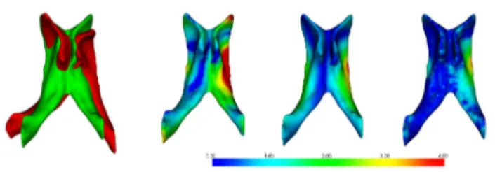
Evaluation. We evaluate the registration error by computing the mean distance between homologous points after registration. The results are reported in Table 1 and an example is displayed in Figure
1. On both anatomical structures, the added value of using fuzziness alone (γ 6= 0, β = 0) is about 35% and of using both fuzziness and affinity (γ, β 6= 0) is about 52% compared to using none (γ, β = 0).
γ, β = 0 γ 6= 0, β = 0 γ, β 6= 0 caudate nuclei 1.64± 1.32 1.12± 0.86 0.78± 0.63
ventricles 2.45± 1.40 1.46± 1.05 1.17± 0.93 Table 1. Experiments on synthetic data (stats). Mean and std (mm) of the registration error for the 10 ventricles and 10 caudate nuclei by varying the fuzziness and affinity parameters.
Fig. 1. Experiments on synthetic data. From left to right: 1) origi-nal (green) and deformed (red) ventricles; 2) mapping of registration error withγ, β = 0 (no fuzziness, no affinity); 3) γ 6= 0, β = 0, (fuzziness, no affinity); 4)γ, β 6= 0 (fuzziness, affinity).
5.2. Results on real data
In the following, we always use the fuzziness term (γ 6= 0). In a first experiment, we evaluate qualitatively the added value of the affinity term i) to map asymmetries [11] of caudate nuclei (whose asym-metries have been related to attention-deficit disorders in children) (Fig 2) and ii) on the registration of the horns of lateral ventricles (Fig 3). We observe that the impact of using the affinity term is es-pecially prominent in areas where crest lines have been detected. In a second experiment, we segment the brain from T1-weighted MRI data of two healthy subjects (300,000 points, brainvisa.info), and we extract four sulcal fundus beds automatically (using our algo-rithm for crest lines) and label them manually for each subject. Then we register the two surfaces i) without using any a priori knowledge (β = 0) and ii) using only 3 out of the 4 sulcal fundus beds to com-pute the affinity function (β 6= 0) (Sec 4.2). The error on the fourth sulcus is used as a quality metric of the registration. It is evaluated to be 7 mm in the first case (β = 0) and 3 mm in the second (β 6= 0). This suggests the usefulness of the affinity term (Fig 4).
Fig. 2. Experiments on real data (caudate nuclei). From left to right: 1) crest lines; 2) asymmetry map without using the affinity term (β = 0); 3) added value of using the affinity term (β 6= 0).
6. CONCLUSION & PERSPECTIVES
We introduced an a priori affinity term in an ICP-like criterion for nonlinear registration of surfaces. We then derived a robust and
Fig. 3. Experiments on real data (inferior and posterior horn of the ventricles). From left to right: initial view of the two surfaces, registration without (β = 0) and with (β 6= 0) the affinity term. Note that the badly segmented third ventricle in one of the surfaces (green) does not influence negatively the registration result.
Fig. 4. Experiments on real data (brain). The four sulci are the central (red), lateral (blue), superior frontal (green) and inferior frontal (yellow) sulci. From left to right: 1) brain 1 (top) and brain 2 (bottom); 2) brain 2 (with sulci shown in transparency) towards brain 1 without using the affinity term; 3) brain 2 towards brain 1 using the constraints on three of the sulci via the affinity term. The fourth - inferior frontal (yellow) - sulcus is better registered using the three others as a constraint.
convergent scheme to minimise this criterion and showed the added value of the new term for registration of various brain structures. The overall algorithm is modular, and other implementation choices could be tested. In particular, the affinity term could be built us-ing other descriptors (with the goal to achieve invariance to affine or more general nonlinear transformations rather than just similarities) or based on probabilistic atlases when available (eg for gyri or sulci) and could be extended to all points instead of only salient points. Moreover, it could be interesting to preserve the line structure of salient lines during the matching process of their points (Step 1).
Acknowledgements -We thank M. Bernard for implementing the extraction of the crest lines and A. Mechouche for labelling the sulci.
7. REFERENCES
[1] M.A. Audette et al. “An algorithmic overview of surface registration techniques for medical imaging,” MedIA, vol. 4, pp. 201–217, 2000.
[2] P.J. Besl and N.D. McKay, “A method for registration of 3-D shapes,” IEEE PAMI, vol. 14, no. 2, pp. 239–256, Dec. 1992.
[3] H. Chui and A. Rangarajan, “A new point matching algorithm for non-rigid registration,” CVIU, vol. 89, no. 2-3, pp. 114–141, 2003.
[4] B. Amberg et al. “Optimal step nonrigid ICP algorithms for surface registration,” IEEE CVPR, pp. 1–8, 2007.
[5] J. Feldmar and N. Ayache, “Rigid, affine and locally affine registration of free-form surfaces,” IJCV, vol. 18, no. 2, pp. 99–119, 1996.
[6] M.A. Fischler and R.C. Bolles, “Random sample consensus: a paradigm for model fitting with applications to image analysis and automated cartography,” Commun. ACM, vol. 24, no. 6, pp. 381–395, 1981.
[7] S. Gumhold et al. “Feature extraction from point clouds,” In Proceedings of the 10 th International Meshing Roundtable, pp. 293–305, 2001.
[8] S. Cha and S.N. Srihari, “On measuring the distance between histograms,” Pat-tern Recognition, vol. 35, no. 6, pp. 1355–1370, June 2002.
[9] A.E. Johnson and M. Hebert, “Using spin images for efficient object recognition in cluttered 3d scenes,” IEEE PAMI, vol. 21, pp. 433–449, 1999.
[10] J.J. Koenderink and A.J. van Doorn, “Surface shape and curvature scales,” Image and Vision Computing, vol. 10, no. 8, pp. 557–564, October 1992.
[11] B. Comb`es and S. Prima, “New algorithms to map asymmetries of 3d surfaces,” MICCAI, New York, USA, pp. 17–25, September 2008.