HAL Id: hal-01730655
https://hal.archives-ouvertes.fr/hal-01730655
Submitted on 13 Mar 2018
HAL is a multi-disciplinary open access
archive for the deposit and dissemination of
sci-entific research documents, whether they are
pub-lished or not. The documents may come from
teaching and research institutions in France or
abroad, or from public or private research centers.
L’archive ouverte pluridisciplinaire HAL, est
destinée au dépôt et à la diffusion de documents
scientifiques de niveau recherche, publiés ou non,
émanant des établissements d’enseignement et de
recherche français ou étrangers, des laboratoires
publics ou privés.
A Local Search Approach to Observation Planning with
Multiple UAVs
Arthur Bit-Monnot, Rafael Bailon-Ruiz, Simon Lacroix
To cite this version:
Arthur Bit-Monnot, Rafael Bailon-Ruiz, Simon Lacroix. A Local Search Approach to Observation
Planning with Multiple UAVs. International Conference on Automated Planning and Scheduling
(ICAPS), Jun 2018, Delft, Netherlands. 9p. �hal-01730655�
A Local Search Approach to Observation Planning with Multiple UAVs
Arthur Bit-Monnot,
1,2Rafael Bailon-Ruiz,
1Simon Lacroix
11LAAS-CNRS, Universit´e de Toulouse, CNRS, France 2DIBRIS, Unitversity of Genoa, Italy
2POLCOMING, University of Sassari, Italy [email protected], {rafael.bailon-ruiz, simon.lacroix}@laas.fr Abstract
Observation planning for Unmanned Aerial Vehicles (UAVs) is a challenging task as it requires planning trajectories over a large continuous space and with motion models that can not be directly encoded into current planners. Furthermore, realistic problems often require complex objective functions that complicate problem decomposition.
In this paper, we propose a local search approach to plan the trajectories of a fleet of UAVs on an observation mission. The strength of the approach lies in its loose coupling with domain specific requirements such as the UAV model or the objective function that are both used as black boxes. Furthermore, the Variable Neighborhood Search (VNS) procedure considered facilitates adaptation of the algorithm to specific requirements through the addition of new neighborhoods.
We demonstrate the feasibility and convenience of the method on a large joint observation task in which a fleet of fixed-wing UAVs maps wildfires over areas of a hundred square kilometers. The approach allows generating plans over tens of minutes for a handful of UAVs in matter of seconds, even when considering very short primitive maneuvers.
Introduction
In the last decade, Unmanned Aerial Vehicles (UAVs) have become a widespread and affordable technology. Fixed-wing UAVs that can reach 50 km/h are now widely available, easy to deploy, maintain and equip. As a result, there is an in-creasing interest in using them for various tasks where more traditional measures would be inconvenient, dangerous or simply costly. Typical examples are Search and Rescue mis-sions in which large and hazardous terrain must be covered while searching for a missing person as well as monitoring or mapping tasks for which a number of observations must be made at several remote locations (Salda˜na et al. 2017; Casbeer et al. 2006; Merino et al. 2012).
In this paper, we case study one such monitoring task in which the objective is to leverage UAVs to perform continu-ous and autonomcontinu-ous mapping of wildfires. The operational constraints of wildfires make the use of UAVs especially ap-pealing: they often occur in remote wooden areas and can rapidly span hundreds of square kilometers. Expected bene-fits are an improvement of the information available to
fire-Copyright c 2018, Association for the Advancement of Artificial Intelligence (www.aaai.org). All rights reserved.
fighters on the field, leading to a safer and more efficient deployment of personnel and resources (Noonan-Wright et al. 2011). Automated or semi-automated information gather-ing is also expected to free up firefighters from undertakgather-ing this task themselves. Indeed, in tension areas where tens of fire can start every day, surveillance is a critical task that monopolizes many firefighters.
Unfortunately, the very reason that makes fixed-wing UAVs appealing for such tasks also renders a full automa-tion difficult. With a typical airspeed of 50 km/h even small and widely available fixed-wing UAVs can cover large areas in a matter of minutes, meaning automated planners must cope with very large continuous search spaces. In addition, such speeds yields kinematic and dynamic constraints – e.g. augmenting the minimum turning radius – that call for more elaborate techniques to compute point to point trajectories. The presence of multiple UAVs further complicates the task at hand, as one must ensure good allocation of tasks among the different agents (Ollero et al. 2005).
In this paper, we formalize a general multi-agent obser-vation problem that captures typical requirements for UAV observation missions. The proposed planning approach is based on Variable Neighborhood Search (VNS), a local search technique that has proved very adapted to solve Ori-enteering Problems and variants with which our observation problems share many characteristics (Vansteenwegen, Souf-friau, and Oudheusden 2011; Geiger et al. 2009).
We show how this technique is instantiated to plan ob-servations of wildfires. In particular, we demonstrate that no adaptation is required to handle specialized point-to-point trajectory planners and complex nonlinear objective func-tions. Despite the very small necessary adaptations, we show that our approach generates good quality plans in a matter of seconds for problems involving multiple UAVs and thou-sands of potential observations to be made over tens of min-utes.
Problem Statement
UAV Model
Here we define a synthetic and generic UAV model whose aim is to abstract the specific details of a given UAV dy-namics, while providing enough information to allow plan synthesis.
Definition 1 (Waypoint) A waypoint is a location in space that a UAV has to reach during the execution of a plan.
Common waypoint representations combine the ground position (x, y, z) in a given frame (e.g. East-North-Up rela-tive to a control tower) and the attitude encoded by a triple (roll, pitch, yaw). Depending on the motion model consid-ered, part of this representation might be kept implicit, for instance the altitude z and the pitch when the UAV is con-strained to stay at a given altitude.
A UAV model implicitly encodes the flight dynamics of a given UAV. The capability needed for planning is the com-putation of trajectories linking two waypoints. Given the en-semble of waypoints W , we require a UAV model υ to pro-vide two functions:
travel-timeυ:W × W → R energyυ:W × W → R
that respectively denote the shortest time needed to go from one waypoint to another and the energy consumption of the resulting trajectory. While not strictly necessary for the pur-pose of planning, the description of the resulting trajectory in space is usually provided as well.
Definition 2 (Maneuver) A maneuver is an elementary tra-jectory of a single UAV.
Maneuvers aim at providing a single interface that ab-stract the differences between subparts of long trajectories. In particular, it can be used to represent single waypoints, straight line flight overs or more complex maneuvers such as spirals or lawnmower patterns that are common when syn-thesizing plans for UAVs.
For a given maneuver m, a UAV model υ provides: • an entry waypoint entryυ(m)∈ W
• an exit waypoint exitυ(m)∈ W • a duration durationυ(m)∈ R
• an energy consumption energyυ(m)∈ R
Definition 3 (Trajectory) A trajectory is a tuple (υ, ts, M ) where, υ is a UAV model, tsis the start time of the trajectory and M = hm1, . . . , mni is a sequence of maneuvers.
For each maneuver mi∈ M, its start time st(mi)and end time et(mi)are computed recursively:
st(m1) = ts
et(mi) = st(mi) +durationυ(mi)
st(mi+1) = et(mi) +travel-timeυ(exitυ(mi),entryυ(mi+1))
The energy consumption of a trajectory is defined as the sum of the consumption of all maneuvers in the trajectory and the energy needed to link any two subsequent maneuvers in the trajectory.
Planning Problem Formulation
Definition 4 (Flight Window) A flight window represents the opportunity for a given UAV to perform an activity sub-ject to certain constraints. A flight window is encoded as a tuple (υ, Mstart, Mend, Tmin, Tmax, E)composed of:
• a UAV model υ
• two sequences of maneuvers Mstartand Mend encod-ing the start and end of any trajectory in this flight win-dow. A simplified application is to specify a single way-point denoting the runway where the UAV must take off and land. More complex settings might consider full trajectories to denote previously executed or currently executing maneuvers.
• a time window [Tmin, Tmax]during which the UAV is allowed to fly.
• the energy E available for the flight window.
We say that a given trajectory (υ, ts,hm1, . . . , mni) is a valid instantiation of a flight window (υ, Mstart, Mend, Tmin, Tmax, E)if:
• hm1, . . . , mni is a feasible sequence of maneuvers for υ.
• the trajectory is fully contained in the allowed temporal interval, i.e., Tmin≤ st(m1)≤ et(mn)≤ Tmax • Mstart and Mend are respectively prefix and postfix
of hm1, . . . , mni; meaning that the trajectory begins and finishes with the maneuvers imposed by the flight window.
• the energy required by the trajectory is no greater than E
Definition 5 (Multi-UAV Observation Problem) A multi-UAV observation planning problem is a tuple (M, F, utility) where M is the set of allowed maneuvers, F is a set of flight windows and utility is a utility function whose input is a set of trajectories and output is a real number.
A plan is a sequence of trajectories. A plan π = ht1, . . . , tki is a solution to a planning problem (M,hf1, . . . , fki, utility) if and only if for each flight window fi, tiis a valid instantiation of fi. A solution plan πis said to be optimal if there exist no solution plan π06= π such that utility(π0)>utility(π).
Observation Planning as VNS
We now introduce a specialized algorithm for solving our observation problem. The proposed approach builds on the Variable Neighborhood Search (VNS) metaheuristic that has been applied to numerous combinatorial optimization problems in Operations Research (Hansen, Mladenovi´c, and Moreno P´erez 2010). VNS algorithms work by repeatedly chaining (i) a descent phase through systematic change of neighborhood providing local improvements to an existing solution; and (ii) a perturbation phase aiming at escaping the valley of the local optimum reached during the descent phase.
One of the key benefits of VNS is its very generic and adaptable definition. Indeed, the descent phase of VNS builds upon a sequence of neighborhoods, where each neigh-borhood typically proposes a local plan adaptation that im-proves a particular aspect of the solution. A simple neigh-borhood could be for instance to swap the order of two se-quenced maneuvers. The fact that each neighborhood is
fo-cused on a particular subtask means they can often be reused when tackling similar problems.
Definitions
Definition 6 (Neighborhood) A neighborhood N defines for each valid plan π a set of neighbor plans N (π) ⊆ Π where Π is the set of valid plans.
A neighborhood is associated with a utility function uN : Π → R giving the utility of a given plan in the context of this neighborhood.
This definition of a neighborhood differs from the usual one by the introduction of the utility function uN which is local to N . For instance, a neighborhood aiming at op-timizing trajectories could base its utility function only on the length of the plan. This choice is motivated by the very general utility function considered for our observation prob-lem. While the problem remains mono-objective, allowing the global objective function to be nonlinear and dependent on the timing of maneuvers makes the generation of use-ful neighbors complex. The neighborhood-dependent utility function allows a greater separation of concerns between the different neighborhoods.
Definition 7 (gen-neighbor) Given a plan π ∈ Π and a neighborhood N , the function gen-neighborN(π) returns either (i) a valid plan π0 ∈ N (π) such that u
N(π0) > uN(π), or (ii) nil if the neighborhood failed to generate an improving neighbor.
Definition 8 (Shuffling) A shuffling function f(π, k) : Π × N→ Π produces a new plan by perturbing the plan π. This perturbation is dependent on k, the current iteration of the search.
Shuffling functions typically apply random changes to the current solution with the objective of escaping local minima.
Variable Neighborhood Search
Our VNS algorithm is depicted in Algorithm 1. It is parame-terized by a sequence of neighborhoods, a shuffling function and a maximum runtime.
Given an initial (possibly empty) partial plan πinit, the descent phase of VNS tries to generate plans improvements by systematically and sequentially trying all neighborhoods hN1, . . . ,Nmi until a neighborhood Ni provides an im-provement. If such an improvement is provided, the current plan is updated and the process restarts from the first neigh-borhood N1. When no neighborhood was able to generate an improvement, the best plan found so far is perturbed by the shuffling function and the descent phase restarts from the first neighborhood N1. This process is repeated until the total runtime goes over the allowed budget tmax, at which point the best plan found is returned.
Neighborhoods
We define two classes of neighborhoods that have proved useful in our setting.
Algorithm 1 A Variable Neighborhood Search (VNS) al-gorithm. VNS takes as parameters an initial plan πinit, a sequence of neighborhoods hN1, . . . ,Nmi, a real tmax in-dicating the maximum planning time and a function shuffle that is applied to the best plan on a restart.
functionVNS(πinit, hN1, . . . ,Nmi, tmax, shuffle) πbest← πinit
num-restarts ← 0 whileruntime ≤ tmaxdo
π← shuffle(πbest,num-restarts)
i← 1 .Select first neighborhood whilei≤ m do
π0
← gen-neighborNi(π)
ifπ0
6= nil then
π← π0 .Update current plan ifutility(π) > utility(πbest) then
πbest← π end if
i← 1 . Switch back to first neighborhood else
i← i + 1 . Switch to next neighborhood end if end while num-restarts ← num-restarts + 1 end while returnπbest end function
Local Path Optimization A local path optimization neighborhood applies a transformation to a single maneu-ver in the plan. The scope of its utility function is limited to the duration and energy consumption of the trajectory.
Typical local path optimization neighborhoods apply a random or deterministic translation or rotation to a single maneuver already in the plan.
Maneuver Insertion A maneuver insertion neighborhood alters a plan by inserting a new maneuver m at a given po-sition in a plan. The quality of a neighbor is assessed by the problem’s utility function, with ties broken by trajectory du-ration or energy consumption.
Maneuver insertion typically works in two phases. First, a new maneuver is generated either systematically or by sam-pling. Second, an insertion location is selected for the ma-neuver, typically the one minimizing the required detour. Given the potentially large number of valid maneuvers, new maneuvers and maneuver transformations are often sam-pled. This approach was proposed by Mladenovi´c et al. (2003) as Reduced VNS to cope with large neighborhoods whose complete enumeration would be computationally ex-pensive.
Other Common Neighborhoods Other common neigh-borhoods in VNS include replacing some of the maneuvers by new ones or swapping maneuvers between two trajecto-ries, e.g. as proposed by Geiger et al. (2009) and Hansen, Mladenovi´c, and Moreno P´erez (2010). However, we found
those to be inefficient in our setting, due to the mostly con-tinuous trajectories in which a maneuver is best considered together with the preceding and following ones. Instead, we rely on shuffling to provide similar benefits (removal of ma-neuvers in trajectories) at a larger scale.
Initial Plan and Shuffling
Our initial plan πinit is built by transforming each flight window (υ, Mstart, Mend, Tmin, Tmax, E)into a trajectory (υ, Tmin,hMstart, Mendi). The initial plan is the aggregation of the resulting trajectories. It is easy to see that such a plan is valid if there exist a solution.
One of the most general shuffling function to complement insertion neighborhoods is the one that randomly retracts a sequence of maneuvers from the current plan. The number of maneuvers to be removed in each trajectory is randomly chosen between 0 and the maximum number of maneuvers that can be removed (i.e. not in the imposed start and end of the trajectory).
Instantiation and Evaluation
Wildfire Monitoring as a Multi-Agent Observation
Problem
We now give an overview of the fire mapping problem on which our VNS approach to observation planning is instan-tiated and evaluated. At the core is a will to take of advantage of fixed-wing UAVs to automate the mapping of wildfires in order to (i) collect images of active fires in real time, (ii) maintain a map of the current fire, and (iii) rapidly confirm and characterize new fire starts.
Fire Map The dynamic nature of wildfires and our desire to allow their autonomous mapping and monitoring calls for some complex data processing. While a complete presenta-tion of the framework is beyond the scope of this paper, we here sketch the main components and their impact on the definition of the planning problem.
A fire mapping problem is characterized by an initial knowledge of the current status of one or multiple wildfires. Such information typically contains a partial history of the position of the fire fronts over time, compiled from past ob-servations. Given this initial knowledge, the objective of a continuous mapping and monitoring system is to maintain a map of the fire over time. For this purpose, the system uses a fleet of fixed-wing UAVs equipped with infrared or regular cameras, and should schedule their observations for the near future (e.g. for the next hour).
The dynamic nature of fires means that the system should be able to predict their evolution in order to know where ob-servations should be made and focus them in the location where the fire is the most dynamic. For this purpose, our system is endowed with fire models (Rothermel 1972; An-derson 1983) that permit the simulation of the fire progress from its last known position, taking into account the envi-ronmental context including the wind, terrain and fuel. The output of this process is a predicted evolution of the fire tak-ing the form of a rasterized map in which each cell is asso-ciated with its time of ignition (if any) as shown in Figure 1.
Figure 1: Fire map showing the expected evolution of a wild-fire spreading over a hilly area from a single ignition point (in red). Background colors reflect the elevation. Level lines denote the expected fire front every 30 minutes. Grey ar-rows represent the local wind field on the ground as given by a local wind simulator for the purpose of simulating the wildfire’s evolution.
In the current implementation of our system, each cell of the fire map is a square with a side of 25 meters.
UAV model Aircraft dynamics are very complex due to aerodynamics, atmospheric conditions and actuator perfor-mance bounds; leading to complex non-linear models. The planning algorithm introduced in this publication only re-quires a lighter UAV model, that doesn’t encompass all the dynamics, but describes its kinematics in a simple yet real-istic manner.
The model we propose is that of a Dubins vehicle. A Du-bins vehicle moves forward at constant speed V and with bounded turn radius |u| ≤ ˙ψmax:
˙ x = V cos(ψ) ˙ y = V sin(ψ) ˙ ψ = u
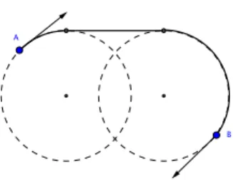
For such vehicles, the work of Dubins (1957) finds opti-mal distance paths between two points with prescribed ori-entation. As shown in Figure 2, those paths are composed of a succession of circular arcs and straight lines. Using Du-bins’ formulations we obtain a good estimate for the exe-cution time of a UAV trajectory at constant altitude. As a result, the waypoint used is a tuple (x, y, ψ) where x and y denote the position relatively to a fixed landmark and ψ is the heading of the UAV which is assumed to fly at a fixed altitude.
Maneuvers The considered maneuvers are short (50 me-ters) straight line trajectories. The rational behind this choice
Figure 2: A Dubins path between two oriented waypoints. Curvature of both circular arcs is given by the maximum turn radius of the UAV.
lies in the limitations of the actual controller for the con-sidered UAVs that supports either waypoint based trajecto-ries or predefined maneuvers such as lawnmower or spirals. While in general adapted to complete area coverage, the lat-ter proved to be unadapted to the given observation task since we are interested in taking pictures of the fire front which, at a given time, is essentially a 2D line. Straight line maneuvers were preferred to simple waypoints to account for the specific constraints of the UAV whose camera points forward and provides more stable images when not turning. The space of maneuvers M is thus defined as the set of segments of fixed length whose center is a cell of the fire map. Even though the fire map is discretized, the segment’s orientation that denotes the angle of approach of the UAV is not and can take an arbitrary value in [0, 2π].
A maneuver m executed at time t is an observation of a given cell c of the fire map if (i) the segment of m is centered on c, and (ii) the fire front is active in cell c at time t. Objective Function The objective function measures the information gathered by a set of UAV trajectories with re-spect to a full knowledge situation. Given C the set of cells ignited during the planning window, our objective is to max-imize the total information gathered over all cells in C:
utility(π) =X c∈C
kl(c, π)
where kl(c, π) associates to each cell c an amount of knowl-edge gathered by a plan π. It is defined through the inverse of the distance from c to the closest observed cell o ∈ π:
kl(c, π) = 1 min
o∈πdist(c, o)
As a result, observing the same cell twice is useless from a utility point of view. Also, the utility brought by a new observation depends on observations already in the plan: if there is already a nearby observation in the plan, its utility will be low. This formulation captures the important spatial correlation of ignition times in the context of wildfires mon-itoring. This correlation can later be exploited to reconstruct fire fronts from observations.1
1More involved definitions of distance (i.e. similarity) based on
fire-related features of cells are also supported by our approach but are beyond the scope of this paper and omitted.
VNS Configuration
Local Path Optimization Neighborhoods We include two local path optimization neighborhoods.
The Ndubneighborhood aims at shortening Dubins trajec-tories by changing the orientation of maneuvers. For a given plan π, a neighbor π0
∈ Ndub(π)is obtained by replacing a maneuver m ∈ π by a new maneuver that only differs by its orientation. The new angle is chosen either randomly or such that the new maneuver is parallel to the line linking the end of the previous maneuver to the start of the next one; as pro-posed by Macharet and Campos (2014). gen-neighborNdub
randomly generates a fixed number of neighbors and returns the first one that reduces the length of the trajectory.
The Nfireneighborhood transforms a maneuver into an ob-servation by translating it on the fire front. Consider a ma-neuver m ∈ π that is not an observation, i.e., the fire front is not in the observed cell at time st(m). Then Nfire(π) con-tains a plan π0where either:
• m is recentered on a neighbor cell in which the fire is active at st(m)
• m is removed from π0. This case is triggered when the fire front is not in a neighbor cell at st(m) or such a neighbor cell is already observed.
Insertion Neighborhoods Insertion neighborhoods work by (i) non-deterministically choosing one maneuver over a yet unobserved cell, and (ii) selecting an insertion location. We define three neighborhoods depending on the strategy for choosing the insertion location:
• Ninsall-bestinserts the sampled maneuver in a plan π such that the overall duration is minimized. All trajectories are considered.
• Nins1-bestinserts the sampled maneuver in a random tra-jectory of π such that the duration of the tratra-jectory is minimized.
• Ninsrandinserts the sampled maneuver at a random loca-tion in the plan.
For all three neighborhoods, gen-neighbor generates a fixed number of neighbors and selects the valid one that has the best utility.
Results
We evaluate our approach on a hundred randomly generated instances of the fire mapping problem. Each instance is a 10 by 7 kilometers area where one to three fire start randomly and spread over 1 hour. Each instance has one to three fixed-wing UAVs with a ground speed of 18 m/s. Each UAV has a flight window of 10 to 30 minutes and is based in a random corner of the area. The code for fire simulation, planning and problem generation is freely available.2
On average the fire front traverses 2243 cells of the fire map during the plan window leading to as many possible observations. Each possible observation can be made from any angle, yielding a virtually infinite number of maneuvers (note that even a coarse discretization of orientation would
yield a very large number of maneuvers). In practice, each UAV can only access about 20% of the possible observations due to the limitation on its flight window.
We evaluate different combinations of neighborhoods and shuffling functions. The score of a solution plan π is given by:
score(π) = utility(π) utility(π∗)
where π∗is the best solution found for the problem instance. Since VNS provides solutions in an anytime fashion, we evaluate the evolution of the score of a given VNS configura-tion over time, e.g., the average score of the soluconfigura-tions found when allowed to plan for 1 second.
We evaluate the following VNS configurations: Name Neighborhoods Shuffling Call-best hNfire,Ndub,Ninsall-besti yes C1-best hNfire,Ndub,Nins1-besti yes Crand hNfire,Ndub,Ninsrandi yes C∗ hNfire,Ndub,Ninsall-best,Nins1-best,Ninsrandi yes Crandno-dubins hNfire,Ninsrandi yes Crandno-shuffling hNfire,Ndub,Ninsrandi no
Table 1: Evaluated VNS configurations.
All configurations first consider local path optimization neighborhoods (Nfireand Ndub). As a result, path optimiza-tion neighborhoods are triggered each time a new inser-tion occurs. The Nfire neighborhood is present in all tested configurations, as omitting it strongly reduced the conver-gence rate. This is because inserting a new maneuver delays later maneuvers, possibly invalidating an observation. The Nfireneighborhood precisely avoids this problem by locally adapting the path to maintain an observation.
Configurations mostly diverge in the definition of the in-sertion neighborhoods from the most involved (Nall-best
ins ) to the simplest (Nrand
ins ). In addition, we introduced a configura-tion C∗that sequentially combines all three insertion neigh-borhoods. The last two configurations aim at illustrating the impact of the Ndubneighborhood and of the shuffling phase. Average scores over the hundred instances are presented in Figure 3 and Table 2. All benchmarks were executed on an Intel Core i5-7200U cadenced at 2.5GHz with a single thread and allowed to run for 30 seconds. As a result of the local search approach taken, memory usage is kept low at all times and is dominated by the encoding of the fire map. On average, the best plan contained 68 observations.
Of the three first configurations (Call-best, C1-best, Crand), Call-best uses the most complex neighborhood. Indeed Ninsall-bestpreselects among all possible insertion locations the one that induces the least detour. As a result, this neighbor-hood favors quality at the expense of diversity. The opposite choice is made for Crand that considers any insertion loca-tion, while C1-bestis a middle ground that considers the best location in a given trajectory.
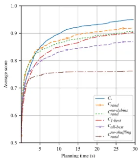
5 10 15 20 25 30 Planning time (s) 0.5 0.6 0.7 0.8 0.9 1.0 A verage score C∗ Crand Cno-dubinsrand C1-best Call-best Cno-shufflingrand
Figure 3: Score of the VNS configurations as a function of the planning time. Score is averaged over all problem in-stances. Time (s) 0.01s 0.1s 1s 10s 30s Call-best .39(.09) .55(.09) .71(.06) .83(.04) .87(.04) C1-best .36(.09) .50(.10) .68(.06) .85(.02) .90(.02) Crand .36(.09) .53(.10) .74(.05) .87(.02) .92(.01) C∗ .39(.09) .55(.09) .71(.05) .90(.01) .95(.01) Crandno-dubins .36(.09) .53(.09) .74(.04) .86(.02) .91(.01) Crandno-shuffling .36(.09) .52(.09) .69(.05) .76(.04) .76(.04)
Table 2: Scores for given planning times, averaged over all problem instances. Best performance is in bold font. Vari-ance is given in parenthesis.
These design choices have direct consequences on per-formance. Call-best is faster at improving its solution during the first second of search, leveraging its high quality neigh-borhood. However this good performance rapidly ends. As the current solution becomes more complex, the low diver-sity in its neighborhood appears to be detrimental. On the other hand, C1-best and Crand both have a slow start up but provide better performance when allowed to plan for over one second, arguably because of the higher diversity in their neighborhoods.
Our C∗ configuration aims at combining the strengths of the different approaches. For this purpose its first insertion neighborhood is Nall-best
ins which allows to quickly build an initial solution by leveraging the high quality of the neigh-bors. However, once Nall-best
ins fails to generate improved so-lutions, C∗falls back to the more diverse N1-best
ins and Ninsrand neighborhoods. This combination allows C∗ to start as fast as Call-best while still outperforming all other approaches in
40 48 48 56 56 56 64 64 64 72 72 72 80 80 80 88 88 88 96 96 96 104 104 104 104 104 104
Figure 4: An example plan with 3 UAVs observing 3 wildfires on a 10 by 5 kilometers area. Our VNS is able to generate plans that balance the information gathering effort between the three agents. In this example, the green UAV arrives early and maps the right-most fire while it is still limited. The red and blue UAVs arrive later and cooperatively map all fires while focusing on the most active areas. Important to note is that this plan was obtained by limiting the planning time to 20ms. With larger planning times, additional maneuvers would have been inserted, resulting in much denser, and less intelligible, trajectories.
(a) With Ndub (b) Without N dub
Figure 5: Typical trajectories found with and without the Ndublocal path optimization neighborhood.
the long run.
As could be expected, preventing the use of shuffling in Crandno-shufflingprevents VNS from escaping the current local op-timum reached during the descent phase. As a result, its overall score quickly stagnates.
More surprising is the overall good performance of Crandno-dubins. In Figure 5, it can be seen that, while the absence of Ndubresults in longer trajectories, this penalty is some-what limited for sparse trajectories. Beside the positive indi-rect effect on the objective function, a subjective yet impor-tant benefit of Ndubis the production of trajectories that are smooth and feel more natural to a human operator.
An example plan is shown in Figure 4. Important to note is that, while having no global knowledge of the task, the combination of VNS neighborhoods generates trajectories that exploit the overall structure of the problem. As a result a team of UAVs is able to follow fire front lines and coop-eratively map wildfires. Essential in this result is the ability to plan with fine-grained maneuvers instead of relying on coarse predefined ones.
Furthermore, only one neighborhood (Nfire) is domain-dependent. While essential for the good performance, its
definition and implementation are kept simple. Overall, the good performance of the system is a result of the combina-tion of simple and mostly generic building blocks.
Related Work
The problem we tackle in this paper features many similar-ities with the Orienteering Problem (OP) of Operations Re-search (Chao, Golden, and Wasil 1996). In the OP, a set of vertices N is associated with a score score : N → R and travel time tt : N × N → R. The objective of the OP is to find a path visiting a subset of the vertices such that the duration of the path is below a predefined time budget and the collected score is maximized. While originating from the sport game of orienteering, it can be used to model observa-tion tasks by interpreting the score as a reward associated with a given observation.
This simple formulation is however restrictive when con-sidering more general observation problems such as our own. In particular, our problem features (i) multiple agents; (ii) a continuous space leading to a potentially infinite num-ber of vertices; and (iii) a more general, possibly nonlinear, utility function. In particular, our very loose definition of the utility function allows to tie the reward associated with a vertex to the time at which it is visited.
Many extensions to the orienteering problem have been proposed that partially tackle those requirements. In partic-ular, the team orienteering problem (Tang and Miller-Hooks 2005) considers multiple agents, the orienteering problem with time windows (Tricoire et al. 2010) constrains the visit of vertices to be in given time windows and the Generalized OP considers nonlinear objective functions (Wang, Golden, and Wasil 2008). Many variants of the OP and approaches to tackle them are presented in the comprehensive survey of Vansteenwegen, Souffriau, and Oudheusden (2011). Most successful approaches are based on existing metaheuris-tics such as TABU search, Genetic Algorithms and
Vari-able Neighborhood Search (Tang and Miller-Hooks 2005; Wang, Golden, and Wasil 2008; Geiger et al. 2009). These approaches were an inspiration in the choice and design of our VNS approach, however none of the surveyed algo-rithms consider our three additional requirements to the OP. In particular none of them was adapted to continuous or very large space for the definition of the vertices.
Classical optimization problems including the OP and the Traveling Salesman Problem have been extended to consider Dubins vehicles (Macharet and Campos 2014; Saska, Faigl, and Petr 2017). The former proposes heuris-tics for finding good orientations of waypoints while the lat-ter relies on graph search to find the best orientations for a sequence of waypoints. Even when considering path op-timization only, the comparison is however limited by the simple waypoints used instead of our more involved maneu-vers. For this reason, our Dubins path optimization neigh-borhood combines a random orientation assignment and a heuristic one by Macharet and Campos (2014)
Some formulations of the Search and Track (SaT) problem also resemble our observation problem. Most work has fo-cused on probabilistic reasoning which is leveraged by a greedy search algorithm over a very short planning horizon (Furukawa et al. 2006; Bourgault, Furukawa, and Durrant-Whyte 2004). Instead, Bernardini, Fox, and Long (2017) transform the problem of searching a target on a road net-work into a deterministic planning problem where the re-ward of observing a given road section depends on the ability of finding the target there. While the resulting prob-lem bears many similarity with the observation probprob-lem con-sidered in this paper, the approach taken is very different. Bernardini, Fox, and Long translate their trajectory planning problem into PDDL2.2 by precomputing a fixed set of spi-ral maneuvers overlapping the road network and the shortest paths between them. This compilation allows them to lever-age domain-independent temporal task planners in a fully automated way. The most important limitation lies in the preprocessing steps that aggressively prunes many solutions from the search space and preselects highly suboptimal neuvers. For instance, the authors only consider spiral ma-neuvers for the observation of straight roads where a simple fly over would have been vastly more efficient.
This approach of decomposing a continuous space into a more manageable subset of large predefined areas and ma-neuvers is considered by other authors (Lin and Goodrich 2014). Instead we do not require any coarse discretization and escape the curse of dimensionality by sampling the pos-sible maneuvers and leveraging point-to-point specialized planners. The use of shuffling and dedicated path optimiza-tion neighborhoods mitigate the shortcomings of sampling while still allowing the use of fine-grained maneuvers as a plan’s build blocks.
Beyond the classical Dubins model that we used to compute point-to-point trajectories, more recent work has focused on providing more expressive and realistic models.
Chitsaz and LaValle (2007) introduce the Dubins airplane that extends the Dubins vehicle with independent altitude control. Using optimal control techniques, they found the
requirements for the shortest Dubins airplane paths between two oriented 3D points. Owen, Beard, and McLain (2015) propose algorithms to generate some paths for the Dubins Airplane – assuming the initial and goal positions are suffi-ciently far – and the control strategy for a fixed-wing UAV to follow them. Another approach to generate paths for the Dubins airplane, that also accounts for initial and goal pitch angles, is introduced by Hota and Ghose (2010).
When wind is considered during flight, the aircraft yaw angle does not correspond to the direction it is heading to. This changes the way of computing trajectories, as the de-picted Dubins paths will get distorted in the presence of wind, without reaching the desired goal. The Dubins vehi-cle model is extended by McGee, Spry, and Hedrick (2005) to deal with this situation. They introduce a strategy to gen-erate Dubins paths in the presence of known arbitrary wind. It models the case as a rendez-vous problem between the aircraft and the goal as a moving target.
Our VNS framework already features an implementation of the Dubins Airplane model which can be used inter-changeably with the 2D version. We also plan to support McGee, Spry, and Hedrick’s extension for wind in order to further increase the realism of the solutions. As long as the computational cost is kept low – as for the two mentioned Dubins’ extensions – we do not foresee any difficulty in sup-porting other motion models in our framework.
Conclusion
In this paper, we have presented an approach to obser-vation planning with multiple UAVs based on Variable Neighborhood Search (VNS). Our problem formulation is kept generic with minimal assumptions on the UAV model, search space and objective function. It is used to encode a wildfire mapping problem in which a fleet of fixed-wing UAVs cooperatively monitor an active wildfire.
The proposed VNS algorithm combines simple build-ing blocks that are mostly domain-independent and easily reusable. Of all the elements in the VNS search only one neighborhood – projection on the fire front – is domain-specific. Even then, the scope of its domain-specific knowl-edge remains contained to a local path optimization. All other components are fully generic and remain simple both in definition and implementation. Each only focuses on a particular subproblem with no knowledge of the global prob-lem apart from black box sampling and utility functions.
Despite its simplicity, we showed our approach to pro-duce good quality plans for a handful of UAVs in a matter of seconds. This is done without any artificial coarse dis-cretization of the search space. Instead, our algorithm han-dles thousands of very primitive maneuvers through a com-bination of sampling and local path optimization. This al-lows us to quickly generate plans that are fine grained even though they span over large areas and long times.
Acknowledgment
This work was partially supported by the FIRE-RS project, within the Interreg Sudoe program co-financed by the Euro-pean Regional Development Fund.
References
Anderson, H. 1983. Predicting Wind-Driven Wild Land Fire Size and Shape. Technical report, USDA Forest Service Research, Research Paper INT-305.
Bernardini, S.; Fox, M.; and Long, D. 2017. Com-bining temporal planning with probabilistic reasoning for autonomous surveillance missions. Autonomous Robots 41(1):181–203.
Bourgault, F.; Furukawa, T.; and Durrant-Whyte, H. F. 2004. Process model, constraints, and the coordinated search strat-egy. IEEE International Conference on Robotics and Au-tomation (ICRA) 5256–5261.
Casbeer, D. W.; Kingston, D. B.; Beard, R. W.; and McLain, T. W. 2006. Cooperative forest fire surveillance using a team of small unmanned air vehicles. International Journal of Systems Science 37(6):351–360.
Chao, I. M.; Golden, B. L.; and Wasil, E. A. 1996. A fast and effective heuristic for the orienteering problem. European Journal of Operational Research 88(3):475–489.
Chitsaz, H., and LaValle, S. M. 2007. Time-optimal paths for a dubins airplane. In 2007 46th IEEE Conference on Decision and Control, 2379–2384.
Dubins, L. E. 1957. On Curves of Minimal Length with a Constraint on Average Curvature, and with Prescribed Initial and Terminal Positions and Tangents. American Journal of Mathematics 79(3):497–516.
Furukawa, T.; Bourgault, F.; Lavis, B.; and Durrant-Whyte, H. F. 2006. Recursive Bayesian search-and-tracking using coordinated UAVs for lost targets. IEEE Inter-national Conference on Robotics and Automation (ICRA) 2006(May):2521–2526.
Geiger, M. J.; Habenicht, W.; Sevaux, M.; and S¨orensen, K. 2009. Metaheuristics for Tourist Trip Planning. Metaheuris-tics in the Service Industry, 624:176.
Hansen, P.; Mladenovi´c, N.; and Moreno P´erez, J. A. 2010. Variable Neighbourhood search: Methods and applications. Annals of Operations Research 175(1):367–407.
Hota, S., and Ghose, D. 2010. Optimal geometrical path in 3d with curvature constraint. In Intelligent Robots and Systems (IROS), 2010 IEEE/RSJ International Conference on, 113–118.
Lin, L., and Goodrich, M. A. 2014. Hierarchical Heuristic Search Using a Gaussian Mixture Model for UAV Coverage Planning. IEEE Transactions on Cybernetics 44(12):2532– 2544.
Macharet, D. G., and Campos, M. F. M. 2014. An Orienta-tion Assignment Heuristic to the Dubins Traveling Salesman Problem. Ibero-American Conference on Artificial Intelli-gence (IBERAMIA) 8864:457–468.
McGee, T. G.; Spry, S.; and Hedrick, J. K. 2005. Optimal path planning in a constant wind with a bounded turning rate. In AIAA Guidance, Navigation, and Control Confer-ence and Exhibit, 1–11. Reston, VA.
Merino, L.; Caballero, F.; Dios, J. R. M. d.; Maza, I.; and Ollero, A. 2012. An unmanned aircraft system for
auto-matic forest fire monitoring and measurement. Journal of Intelligent and Robotic Systems 65(1):533–548.
Mladenovi´c, N.; Petrovi´c, J.; Kovaˇcevi´c-Vujˇci´c, V.; and ˇCangalovi´c, M. 2003. Solving spread spectrum radar polyphase code design problem by tabu search and variable neighbourhood search. European Journal of Operational Research 151(2):389–399.
Noonan-Wright, E. K.; Opperman, T. S.; Finney, M. A.; Zimmerman, G. T.; Seli, R. C.; Elenz, L. M.; Calkin, D. E.; and Fiedler, J. R. 2011. Developing the US Wildland Fire Decision Support System. Journal of Combustion.
Ollero, A.; Lacroix, S.; Merino, L.; Gancet, J.; Wiklund, J.; Remuss, V.; Veiga, I.; Gutierrez, L. G.; Viegas, D. X.; A.Gonzalez, M.; Mallet, A.; Alami, R.; Chatila, R.; Hom-mel, G.; Colmenero, F. J.; Arrue, B.; Ferruz, J.; Martinez, J. R.; and Caballero, F. 2005. Multiple eyes in the sky: Ar-chitecture and perception issues in the comets unmanned air vehicles project. IEEE Robotics and Automation Magazine 12(2):46–57.
Owen, M.; Beard, R. W.; and McLain, T. W. 2015. Im-plementing dubins airplane paths on fixed-wing UAVs. In Valavanis, K. P., and Vachtsevanos, G. J., eds., Handbook of Unmanned Aerial Vehicles. Springer Netherlands. 1677– 1701.
Rothermel, R. C. 1972. A mathematical model for predict-ing fire spread in wildland fuels. Technical Report INT-115, USDA Forest Service Research Paper INT USA.
Salda˜na, D.; Ani Hsieh, M.; Campos, M.; Kumar, V.; and Martins, A. 2017. Cooperative prediction of time-varying boundaries with a team of robots. In International Sympo-sium on Multi-Robot and Multi-Agent Systems (MRS). Saska, M.; Faigl, J.; and Petr, V. 2017. Dubins Orienteering Problem. IEEE Robotics and Automation Letters 2(2):1210– 1217.
Tang, H., and Miller-Hooks, E. 2005. A TABU search heuristic for the team orienteering problem. Computers and Operations Research 32(6):1379–1407.
Tricoire, F.; Romauch, M.; Doerner, K. F.; and Hartl, R. F. 2010. Heuristics for the multi-period orienteering problem with multiple time windows. Computers and Operations Re-search 37(2):351–367.
Vansteenwegen, P.; Souffriau, W.; and Oudheusden, D. V. 2011. The orienteering problem: A survey. European Jour-nal of OperatioJour-nal Research 209(1):1–10.
Wang, X.; Golden, B. L.; and Wasil, E. A. 2008. Using a Genetic Algorithm to Solve the Generalized Orienteering Problem. The Vehicle Routing Problem: Latest Advances and New Challenges 263–274.