Characterization of structural properties and dynamic behavior using distributed accelerometer networks and numerical modeling

(1)

Characterization of Structural Properties and Dynamic Behavior

using Distributed Accelerometer Networks and Numerical Modeling

by

Peter Adam Trocha

Bachelor of Science in Civil Engineering Carnegie Mellon University, 2011

OF TECHNOLOGY

JUL 0

8 2013

.LIBR ARIES

SUBMITTED TO THE DEPARTMENT OF CIVIL AND ENVIRONMENTAL ENGINEERING IN PARTIAL FULFILLMENT OF THE REQUIREMENTS FOR THE DEGREE OF

MASTER OF SCIENCE IN CIVIL AND ENVIRONMENTAL ENGINEERING AT THE

MASSACHUSETTS INSTITUTE OF TECHNOLOGY JUNE 2013

Signature of Author_

Department of Civil and Environmental Engineering May 10, 2013

Certified by_

Eduardo Kausel Professor of Civil and Environmental Engineering Thesis Supervisor

'1 _A

Acepedbyi

Heidi M. liepf Professor of Civil and Environmental Engineering Chair, Departmental Committee for Graduate Students

(2)

(3)

Characterization of Structural Properties and Dynamic Behavior using

Distributed Accelerometer Networks and Numerical Modeling

by

Peter Adam Trocha

Submitted to the Department of Civil and Environmental Engineering on May 10, 2013 in Partial Fulfillment of the

Requirements for the Degree of Master of Science in Civil Engineering

ABSTRACT

Both vibration-based structural health monitoring methodologies and seismic performance analysis rely on estimates of the base-line dynamic behavior of a structure. A common method for making this estimate is through measuring structural motions using sensors deployed in the structure of interest. This procedure was applied to the Green Building, a 20 story structure on the campus of the Massachusetts Institute of Technology. Using a network of 36 accelerometers installed in the structure by the United States Geological Survey, the response accelerations from ambient vibrations, seismic loading, and firework excitations were collected. Spectral analysis methods were applied to the collected data to identify the frequencies and general mode shapes of eight normal modes of the structure. These frequencies were 0.68 Hz, 2.45 Hz, and 8.10 Hz in the east-west direction; 0.75 Hz, 2.85 Hz, and 8.25 Hz in the north-south direction; and 1.45 Hz and 5.05 Hz in torsion. The building was found to have strong torsional responses, an asymmetry in the dynamic behavior of the eastern and western sides, and substantial base rocking motion, even under ambient excitations. Using the original design documents, the Green Building was numerically modeled with a lump-mass stick model and a mixed-element beam-shell finite element model. These models were validated and refined using the collected acceleration data. Initial simulations of seismic excitations demonstrated both models to have good agreement with measured values. The numerical models and structural characterization of the Green Building will be used to further develop vibration-based damage detection methodologies and to predict structural performance during strong seismic events.

Thesis Supervisor: Eduardo Kausel

(4)

(5)

Acknowledgements

My thanks go to a number of people and organizations who have made this work and my study at MIT possible.

First and foremost, I would like to thank my thesis supervisor, Professor Eduardo Kausel, for his guidance, tremendous insight, patience, and support. I am deeply grateful for the opportunity to have worked with him. I would also like to thank Professor Oral Buyukozturk for his help, advice, and encouragement. I am especially indebted to fellow graduate student Justin Chen for always lending a helping hand and sharing his extensive experience and keen advice. Special thanks go to Shell Oil, which has made this project possible through their generous funding.

My love and gratitude go out to my parents, Adam and Anna Trocha, who have supported me over the years and provided unremitting care and encouragement. Without them, none of this would have been possible.

I'd like thank MIT's Catholic Community and the FOCUS team for making Boston and MIT feel like home. Their fellowship, moral guidance, and support have been invaluable. Finally, I am grateful to the many people I have encountered over the years, at MIT and elsewhere, who have extended their friendship and help. There are too many to mention here, but to start, many thanks go to Neel, Kevin, and my roommate, Sakul. In particular, my deep gratitude goes to Bharath, Lucas, Victor, Nate, Mathew, and Maita. I consider myself blessed to have known you.

(6)

(7)

List of Figures

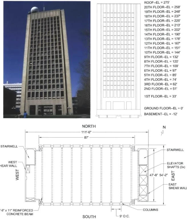
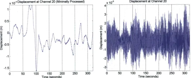
Figure 2-1: Elevation and plan views of the Green Building; (Top Left) photograph of the Green Building's south fagade; (Top Right) elevation view of the south fagade; (Bottom) plan view of a typical floor in the G reen B uilding ... 2 1 Figure 2-2: Distribution and orientation of USGS accelerometers within the Green Building ... 23 Figure 2-3: Accelerometer and data recorder; (left) Episensor ES-US Accelerometer; (right) Granite data recorder (not to scale) ... 2 3 Figure 3-1: The frame test applied to an ambient acceleration time history recorded at Accelerometer 26. ... 2 6 Figure 3-2: Colormap plot of Green Building accelerations in the NS direction due to the 10/16 Hollis C enter E arthquake ... ₃₃ Figure 4-1: Comparison of displacement time histories from a minimally processed signal (left) and from a filtered and base-lined signal (right)... 34 Figure 5-1: Acceleration time-history at the 2nd floor of the Green Building (NS direction) resulting from

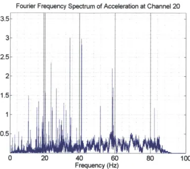
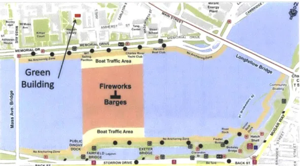
am bient excitation on June 22, 2012... 38 Figure 5-2: Fourier spectrum of ambient vibrations at Channel 20 showing high frequency noise ... 39 Figure 5-3: Acceleration time histories from the ground floor of the Green Building (EW Direction), resulting from an unidentified excitation on May 14, 2012; (right) detail of the event...40 Figure 5-4: Fourier spectrum of May 14 event vibrations at Channel 20 showing high frequency noise ..41 Figure 5-5: Location of fireworks barges for Boston's 4th of July fireworks show ... 42

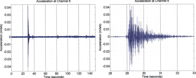
Figure 5-6: Acceleration time histories from the second floor of the Green Building (NS Direction) during Boston's 4th of July fireworks show; (left) full time history; (right) detail of the show beginning ... ₄₂

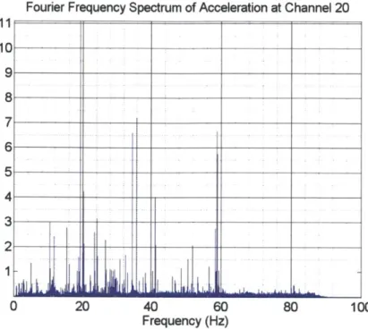
Figure 5-7: Fourier spectrum of 4th of July fireworks induced vibrations at Channel 20; larger than usual am ount of high frequency content is visible ... 43 Figure 5-8: Location of the 10/16 Hollis Center Earthquake... 44 Figure 5-9: Ground response at ground-level NS direction (Station 9) with a detail (right)... 44 Figure 5-10: Fourier spectrum of the Hollis Center earthquake; from a recording taken at ground level in th e N S d irection ... 4 5 Figure 5-11: Fourier spectrum of the Hollis Center earthquake; from a recording taken at the 7th floor in

(11)

Figure 6-1: Fourier spectra of accelerations occurring during the 6/22 ambient vibration recording. The top row shows recordings in the EW (left) and NS (right) directions on the eastern side of floor 19, while the bottom row show s the sam e plots at floor 12... 49 Figure 6-2: Coherences of NS oriented accelerometers paired against the floor 19 sensor; from the 6/22 ambient vibration. Note the positive coherence at 0.75 Hz and 1.45 Hz... 50 Figure 6-3: Coherences of EW oriented accelerometers paired against the floor 19 sensor; from the 6/22 ambient vibration. Note the positive coherence at 0.68 Hz ... 51 Figure 6-4: Coherences of parallel pairs of NS oriented accelerometers from the 6/22 ambient vibration recording. The negative coherence at 1.45 Hz indicates a torsional mode. ... 51 Figure 6-5: Fourier spectra of accelerations occurring during the Fourth of July fireworks show. The top row shows recordings in the EW (left) and NS (right) directions on the eastern side of floor 19, while the bottom row show s the sam e plots at floor 12... 52 Figure 6-6: Fourier spectra of accelerations occurring during the May 14 event. The top row shows recordings in the EW (left) and NS (right) directions on the eastern side of floor 19, while the bottom row show s the sam e plots at floor 12. ... 53 Figure 6-7: Coherences of NS oriented accelerometers paired against the floor 19 sensor; from the May 14 event. Note coherences at 2.85 Hz suggesting a cross-over point ... 55 Figure 6-8: Coherences of EW oriented accelerometers paired against the floor 19 sensor; from the May 14 event. Note coherences at 2.45 Hz suggesting a cross-over point, and the coherence separation at 5.05 H z ... 5 5 Figure 6-9: Coherences of parallel pairs of NS oriented accelerometers from the May 14 event. The strong positive coherence at 2.85 Hz suggests a NS m ode ... 56 Figure 6-10: Power spectra of accelerations occurring during the May 14 event. The top row shows recordings in the EW (left) and NS (right) directions on the eastern side of the roof level, while the bottom row show s the sam e plots at floor 12... 58 Figure 6-11: Detail of coherences of NS oriented accelerometers paired against the floor 7 sensor; from the May 14 event. Note coherence distribution around 8.25 Hz... 59 Figure 6-12: Detail of coherences of EW oriented accelerometers paired against the floor 7 sensor; from the May 14 event. Note separation of coherences around 8.2 Hz... 59 Figure 6-13: Distribution of vertical accelerometers in the Green Building's basement level...60 Figure 6-14: Base Rocking in the Green Building; along the NS and EW axis (left and center). Rocking consists of a rigid-body rotation (exaggerated) and pile uplift and sinking (right) ... 60 Figure 6-15: Fourier frequency spectra of the vertical base accelerometers subjected to the 4th Of July

(12)

Figure 6-16: Coherence between vertically-aligned accelerometers in the basement of the Green Building subjected to the 4h of July firew orks show ... 63

Figure 6-17: Detail of coherence between vertically-aligned accelerometers in the 0-2 Hz range ... 63 Figure 6-18: Cumulative spectral power at floor 12 during June 22 ambient vibrations (left) and the May 14 event (right). Note the steep rises around 1.45 Hz and 5.05 Hz. ... 65 Figure 6-19: Cumulative spectral power at floor 19 during the May 14 event. The sharp rise at 1.45 Hz dem onstrates the contribution of torsional m otion... 66 Figure 6-20: Accelerations from ambient vibrations (top) and the Hollis Center earthquake (bottom) at floor 12. Recordings from NS oriented accelerometers on the East side (left) and West side (right)...68 Figure 6-21: Noise levels at floor 18 due to ambient excitation. Comparison between NS oriented accelerometers located at opposite sides of the floor (left) and between NS and EW oriented accelerom eters at the eastern side ... 69 Figure 7-1: 3D solid model of the Green Building; (left) view from above; (center) view from below;

(right) w ith shear walls and floor slabs rem oved... 72 Figure 7-2: Lumping of Green Building properties for the lumped-mass stick model. The mass of each floor is modeled as a point mass (represented on the right as a circle with an 'm#' annotation), while the story stiffness are modeled as equivalent beams (represented on the right by the 'k#' annotated lines connecting the m asses) ... 73 Figure 7-3: The modal damping ratio as a function of frequency for the Green Building lumped mass model; (left) the damping ratio at low frequencies; (right) damping ratios at high frequencies...76 Figure 7-4: Green Building floor with equivalent beam element ... 77 Figure 7-5: Set-up for lumping of mass and stiffness properties of a Green Building floor to an equivalent lum ped-m ass elem ent...79

Figure 7-6: The condensation of a floor stiffness matrix of a full finite element model to the 6x6 equivalent stiffness matrix used in the lumped-mass model... 81 Figure 7-7: Finite element floor model of a typical floor in the Green Building. Lines represent beam e lem en ts...8 2 Figure 7-8: Accelerations at the Green Building roof level (NS axis) due to the Hollis Center Earthquake as predicted by the lum ped m ass m odel... 85 Figure 7-9: Recorded accelerations at the Green Building roof level (NS axis) due to the Hollis Center E arth q u ak e ... 8 5 Figure 7-10: Meshed beam-shell finite element model of the Green Building... 87

(13)

Figure 7-11: Comparison between predicted and measured Green Building displacements at roof level (NS axis) due to the Hollis Center Earthquake; (left) as predicted by the beam-shell model and (right) as

m easured by accelerom eters ... 88

Figure A-1: Distribution of accelerometers in the Green Building, labeled by channel number...93

Figure B-1: Distribution of accelerometers in the Green Building, labeled by channel number...100

Figure C-1: Distribution of accelerometers in the Green Building, labeled by channel number... 107

Figure D-1: Distribution of accelerometers in the Green Building, labeled by channel number...114

Figure E-1: Solid model of the ground floor of the Green Building (top view) ... 121

Figure E-2: Solid model of the ground floor of the Green Building (bottom view)... 121

Figure E-3: Solid model of the first floor of the Green Building (top view)... 122

Figure E-4: Solid model of the first floor of the Green Building (bottom view)... 122

Figure E-5: Solid model of a typical floor of the Green Building (top view)... 123

Figure E-6: Solid model of a typical floor of the Green Building (bottom view)... 123 Figure F-1: Finite element model of the Green Building ground floor. Wireframe (left) and 3D visual

(rig h t) ... 12 4 Figure F-2: Finite element model of the Green Building first floor. Wireframe (left) and 3D visual (right)

... 1 2 4 Figure F-3: Finite element model of the Green Building typical floor. Wireframe (left) and 3D visual

(14)

List of Tables

Table 3-1: Criteria for stationary and ergodic processes. E is some statistical moment, f and g are two time

histories sampled from the same ensemble, and ti and t2 are two arbitrary times ... 25

Table 3-2: Rules of thumb for interpreting correlation values... 30

Table 5-1: Peak accelerations in the NS, EW, and vertical directions due to ambient excitation ... 38

Table 5-2: Peak accelerations in the NS, EW, and vertical directions due to the 5/14 Event excitation .... 40

Table 5-3: Peak accelerations in the NS, EW, and vertical directions from the July 4th fireworks show...42

Table 5-4: Peak accelerations in the NS, EW, and vertical directions due to the 10/16 earthquake ... 45

Table 6-1: Natural frequencies of the Green Building identified using data from the accelerometer array48 Table 6-2: Ratios between the observed second and first normal modes of the Green Building ... 56

Table 6-3: Peak displacements at the vertical accelerometers ... 64

Table 6-4: Comparison of peak accelerations between parallel NS oriented accelerometers at floor 18 due to v ariou s ex citation s ... 69

Table 7-1: Material properties applied to the solid and FE models of the Green Building. These values correspond to high strength structural concrete ... 82

Table 7-2: M ass properties of a typical floor ... 83

Table 7-3: Comparison between lumped-mass model modal frequency predictions with those determined using the Green Building accelerom eter data ... 84

Table 7-4: Comparison of beam-shell model modal frequency predictions with those determined using the G reen B uilding accelerom eter data...87

Table A-1: Summary of 6/22 ambient vibration recording... 93

Table B-1: Sum m ary of M ay 1 4th event recording ... 100

Table C-1: Sum m ary July 4th fireworks show recording ... 107

Table D-1: Summary of Hollis Center earthquake recording ... 114

Table G-1: 6x6 equivalent stiffness matrix of the Green Building ground floor for the lumped mass model ... 1 2 5 Table G-2: 6x6 equivalent stiffness matrix of the Green Building first floor for the lumped mass model ... 1 2 5 Table G-3: 6x6 equivalent stiffness matrix of the Green Building typical floor for the lumped mass model ... 1 2 5 Table H-1: 6x6 mass matrix of the Green Building ground floor for the lumped mass model ... 126

Table H-2: 6x6 mass matrix of the Green Building 1Vt floor for the lumped mass model... 126

(15)

(16)

1 Introduction

1.1 Motivation and Background

The work contained in this thesis is part of a part of larger project into structural damage detection using distributed sensor networks funded by the Shell Oil Company. It is a collaboration between Shell Oil, Draper Laboratory, the MIT Computer Science and Artificial Intelligence Laboratory (CSAIL), and the MIT Department of Civil and Environmental Engineering (CEE). The goal of this project is to develop a sensor-based damage detection system which specifically tackles the problems of damage detection methodologies, sparse sensor availability, and novel sensing methods. The tasks for accomplishing this goal include investigation of structural health assessment methods based on material and structural behavior, design of reliable and cost-effective sensor networks, development of algorithms for sensor placement optimization and data inferencing, and field testing of a sensor system on a campus building. The study presented in this thesis seeks to identify the vibrational characteristics of a unique structure located in Cambridge, Massachusetts and to create predictive numerical models of its dynamic behavior. This corresponds to the project goals by demonstrating and developing the feasibility of vibration based damage detection in large civil structures using accelerometer sensors, by establishing a base-line understanding of a structure's dynamic properties in anticipation of future field-testing, and by creating numerical models which can be used for both testing of algorithm testing and as tools for damage detection. A secondary motivation for this study is to characterize the dynamic behavior of a structure in the New England region, in the context of seismic performance.

Damage detection is a central concern of structural health monitoring (SHIM). The objective of SHM is to use emergent sensing technologies, coupled with knowledge of material and structural properties, to infer the physical condition of a structure. Damage detection specifically seeks to detect, localize, and estimate the degree of damage sustained by a structural system. The damage can be long-term, .such as corrosion, or a short-term event, such as a sudden member failure. SHM damage detection technologies are especially pertinent given the large quantity and poor maintenance condition of critical infrastructure systems-such as bridges and dams-found in the United States and other countries. SHM is also highly useful in structures where human access is difficult or dangerous-such as nuclear facilities, lengthy pipelines, or off-shore oil platforms. The benefits of SHM and damage detection include reducing the need, cost, and risks incurred by human inspections of structural systems; increasing the lifetime of structural systems by easing the detection of degradation; and preventing the economic, human, and national security damage caused by failure of infrastructure systems and other structures.

(17)

Many approaches exist for SHM, but one early-developed and robust method is vibration based damage detection. This technique is founded on the axiom that changes to a structure's stiffness or mass will result in detectable shifts in its vibrational properties. Specifically, the structure's natural frequencies, mode shapes, and modal damping ratios can be used as parameters for damage detection (Alvandi & Cremona, 2005), (Salawu, 1997). The use of natural frequencies is especially attractive since they can be easily acquired using accelerometer networks and efficiently computed. These modal parameters can also be used for damage localization and evaluation, since different locations and degrees of damage have different effects on the locations and modes of the structure. It is possible to couple this behavior with numerical model updating or subset selection algorithms to determine specific scenarios of damage which may be responsible for the observed property shifts. The accuracy of these approaches is, to an extent, driven by the density and resolution of the sensor arrays. Data inferencing can be used to increase the amount of information provided by sparse sensor networks. A basic, though not necessarily elegant, method for accomplish this is through coupling sensor measurements with numerical models to predict structural responses at un-sampled locations.

The second motivation of this study is to characterize the vibrational properties of a structure in the New England region, particularly in response to seismic loading. Boston and most of New England lie in a "moderate" earthquake hazard zone, which means that the area can experience level VI events on the Modified Mercalli Intensity Scale. The New England region rests on top of old continental crust which was substantially stressed by continental rifting during the Mesozoic era. This created many ancient faults which are difficult to locate and whose seismic activity is nearly impossible to predict (Kafka, 2011). Furthermore, large areas of Boston and Cambridge are built on fill material which may amplify ground motion during seismic events (Britton, et al., 2002). It is unclear what effect these geological features would have on buildings in the greater Boston area, should a stronger earthquake strike the region. In the past two years, two earthquakes have been felt in the Boston area. In 2011, a 5.8 magnitude earthquake occurred near Richmond, Virginia, and it was felt at Level VII in Boston. In 2012, a 4.0 magnitude earthquake occurred near Hollis Center Maine.

By determining a structure's dynamic characteristics, such as natural frequencies, mode shapes, damping, and deflections, it is possible to estimate its general response to seismic excitations and the damage it may experience (Celebi, 2007). The finite element method is valuable in this regard, since it can be used to perform dynamic simulations of seismic events on numerical representations of the structure. Information about the dynamic characteristics of local structures is particularly useful in New England, since very few buildings in the area have been evaluated in this manner for their seismic response behavior. Given an understanding of a structure's seismic performance, the results can be extended to other similar buildings in the region.

(18)

1.2 Objectives and Approach

The general objectives of the work undertaken in this thesis are to characterize the dynamic behavior of the Green Building-a structurally unique building on the Cambridge, Massachusetts campus of the Massachusetts Institute of Technology-and to develop computational models by which this behavior can be predicted. The overarching purpose is to demonstrate and further develop vibration based methods for structural damage detection, with the secondary purpose of discovering vibrational properties which can be used for a seismic evaluation of a Boston area structure. The specific goals to accomplish these objectives are fourfold and include the following:

1. To determine several natural frequencies of the Green Building and to estimate their corresponding mode shapes.

2. To identify features of dynamic behavior and link these to structural and geotechnical design choices

3. To represent the Green Building using a finite element numerical model which accurately predicts the structure's dynamic characteristics

4. To demonstrate the use of distributed sensors networks to characterize and monitor a structure's behavior, and to motivate the use of such systems for structural damage detection

Goals 1 and 2 will be accomplished in part by using a sensor array of 36 accelerometers installed in the Green Building by the United States Geological Survey (USGS). The system will be used to record building motions in response to various excitations. The resulting data will be analyzed using classical spectral analysis methods-such as Fourier analysis, power spectrum, and coherency spectrum-as well as other methods to locate natural frequencies and estimate deflection shapes. A comparative analysis using these methods will also help determine novelties in building motions, which can then be linked to known structural features. Goal 3 will be accomplished by using the building's design documents and standard finite element techniques to create numerical models of the Green Building. The frequencies and motion characteristics from Goals 1 and 2 will then be used to validate and refine the models as necessary. Goal 4 will proceed from successful completion of Goals 1, 2, and 3.

1.3 Thesis Organization

This thesis can be divided into three sections, each of which addresses part of the first three goals-background material and theory (Chapters 2 to 4), sensor data collection and analysis (Chapters 5

and 6), and development of numerical models (Chapter 7). The contents of each chapter in this thesis are briefly summarized below.

(19)

* Chapter 1: Introduction

Presents background information and motivations for the research work * Chapter 2: Physical Assets

Describes the campus building (Green Building) under study and the capabilities of the accelerometer network used for data collection

" Chapter 3: Time Series Analysis Methods

Reviews the basic theory and methods for analyzing the time-series data collected using the accelerometer array

* Chapter 4: Data Pre-Processing

Presents some of the signal processing methods-such as filtering and base-lining-applied to the collected data

* Chapter 5: Collected Data Sets

Summarizes the recorded accelerometer data sets and their corresponding excitations * Chapter 6: Feature Identification

Describes the application of the analysis methods from Chapter 3 to the data sets listed in Chapter 5, and presents the Green Building's natural frequencies, structural behaviors, and other observed results

e Chapter 7: Green Building Modeling

Outlines the theory and process for creating a lumped-mass stick model and a mixed element beam-shell finite element model of the Green Building; presents initial validation results

* Chapter 8: Future Work and Applications

Proposes areas of future work and possible applications of the research carried out * Chapter 9: Conclusions

(20)

2 Physical Assets

2.1 The Green Building

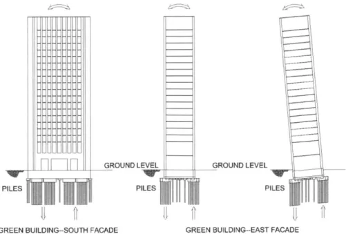
Characterization studies of structural properties and dynamic behavior focused on the Green Building, also known as Building 54. The Green Building is an academic building on the campus of the Massachusetts Institute of Technology in Cambridge, Massachusetts. It is home to the lab, office, and classroom space of the Department of Earth and Planetary sciences. The Green Building was designed by I.M. Pei and constructed between 1962 and 1964. It is currently the tallest building in Cambridge. The roof supports radio and meteorological equipment, including a weather radar system enclosed within a large radome.

The Green Building is 83.7 m (274'-9") tall with a footprint of 16.5 x 34 m (54' x 111'). The

short edges of the building are aligned at about 25' north-west. Henceforth, the short and long directions of the Green Building will be referred to as North-South and East-West (NS and EW), respectively. The building has 21 stories and a below-grade basement level which connects to the MIT tunnel network at the South-West and North-East corners. The first floor is 10 m above grade and houses a large lecture hall. The inter-story height of the first two floors is about 7.8 m, while that of the remaining floors is 3.5 m. Mechanical rooms are located on the top two floors, and the heavy meteorological and radio equipment mentioned above is asymmetrically mounted on the roof. The radome is on the south-west corner. Three elevator shafts are located on the eastern side of the building, while the building's two stairwells are placed symmetrically at the North-East and North-West corners. The elevator shafts insert large voids, measuring about 9.75 x 2.21 m (32' x 7.25'), into the otherwise continuous floorslabs. The elevator shafts (and associated void-space) run the height of the building. The footprint of each stairwell is about 4.27 x 2.29 m (14' x 7.5'). The building is constructed of cast-in-place reinforced concrete with two compressive strengths of concrete used. Interior beams, slabs, and stairs are composed of 3750 psi concrete while all other components are constructed from 4000 psi concrete. The Eastern and Western facades are composed of 0.25 m (10") thick shear walls which run the height of the building. Floor slabs are typically 0.10 16 m (4") thick. Figure 2-1 shows the elevation of the Green Building and a typical floor plan.

The foundation system consists of footings supported by 14" diameter circular piles with pile caps. The piles are part of a floating foundation system and each has a capacity of 50 tons. The basement floor elevation is 3.8 m (12 ft. 6 in) below grade, and grade level is about 6.1 m (20 ft.) above sea level and 36.6 - 40.1 m (120 - 130 ft.) above bedrock (Celebi, et al., 2013). The site is adjacent to the Charles

(21)

River Basin and it is primarily composed of fill material. Geotechnical investigations of the area have found the fundamental site frequency to be about 1.5 Hz. (Celebi, et al., 2013).

V NORTH ROOF-EL = 275' 20TH FLOOR--EL = 258' 19TH FLOOR--EL = 248' 18TH FLOOR--EL = 237' 17TH FLOOR--EL = 225' 16TH FLOOR--EL = 213' 15TH FLOOR--EL = 202' 14TH FLOOR--EL = 190' 13TH FLOOR--EL = 178' 12TH FLOOR--EL = 167' 11TH FLOOR--EL = 151' 10TH FLOOR--EL = 144' 9TH FLOOR--EL = 132' 8TH FLOOR--EL = 120' 7TH FLOOR--EL = 109' 6TH FLOOR--EL = 97' 5TH FLOOR--EL = 85' 4TH FLOOR-EL = 74' 3RD FLOOR--EL = 62' 2ND FLOOR--EL = 51' 1ST FLOOR--EL = 33' GROUND FLOOR-EL = 0' BASEMENT-EL = -12' N 111'-6" 87' STAIRWELL STAHRWEL WEST _ELEVATOR SHEAR WALL SHAFTS (3x) 47'-8" 54'-2" EAST SHEAR WALL 3'-6" x 11" REINFORCED COLUMNS CONCRETE BEAM SOUTH 9' O.C.

Figure 2-1: Elevation and plan views of the Green Building; (Top Left) photograph of the Green Building's south faeade; (Top Right) elevation view of the south faeade; (Bottom) plan view of a typical floor in the Green

Building

(22)

2.2 Green Building Accelerometer Array

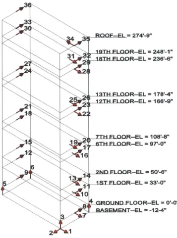
The Green Building is instrumented with 36 uniaxial EpiSensor ES-US force balance accelerometers produced by Kinemetrics. These sensors are designed primarily for structural monitoring purposes. The accelerometer placement and orientations are shown in Figure 2-2. This array and the associated data recording system have been in operation since October 2010, and they are the property of the USGS. Each sensor collects 200 samples per second with a recording range of ±4g. The accelerometers are cable-connected to a central data recording station and time-synchronized using GPS-accurate to within 1 microsecond. The data recorder is the Granite model, also produced by Kinemetrics. The system is internet-connected and set to trigger if accelerations over 1 gal (1 cm/s2) are detected. Acceleration data can also be collected through on-demand recordings and real-time streaming. An EpiSensor accelerometer and a Granite data recorder are pictured in Figure 2-3. The array is designed to monitor translations in the NS and EW directions, torsion, and base rocking motion. Torsional behavior is measured using parallel, NS-oriented sensors located at opposite ends of instrumented floors, while base rocking is determined using the four vertically aligned accelerometers in the basement. It is also possible to calculate floor drift ratios using vertically parallel accelerometer pairs. The displacement and velocities of each sensor can be calculated by numerical or frequency-domain integration, coupled with appropriate filtering to remove artifacts. The sensor system continuously records building motion and stores acceleration data in an adjustable buffer for 5 days.

To prevent aliasing, the incoming data is digitally filtered at the recorder by several Finite Impulse Response (FIR) filters (Kinemetrics, 2008). Accelerometer data is collected in 1 second packets and output in MATLAB .m files as raw ADC counts across a 24 bit range. Equation (2.1) is used to convert the raw ADC counts to engineering units. The installed accelerometers operate on ±2.5 volt range and a sensitivity of 0.625 V/g. If converting to units of m/s2

, Equation (2.1) reduces to Equation (2.2).

ii = (Raw ADC) * (Voltage Range) (Gravitational Accleration) (2.1) (ADC Scale)(Sensativity)

(2.5)(9.81) _

U(m/s2) = (Raw ADC) * (=.5)(.2) _ (Raw ADC)(4.678 * 10-6) (2.2)

(23)

Figure 2-2: Distribution and orientation of USGS accelerometers within the Green Building

Figure 2-3: Accelerometer and data recorder; (left) Episensor ES-US Accelerometer; (right) Granite data recorder (not to scale)

(24)

3 Time Series Analysis Methods

Due to the complexity of the system under study, the presence of random noise, and numerous measurement uncertainties, the collected Green Building accelerometer time histories were analyzed using statistical and spectral methods. These time histories belong to a class of random, or stochastic, processes, to which a brief introduction is found in Section 3.1. The remainder of this chapter will present an overview of the analysis techniques applied to the Green Building data. However, detailed estimator procedures and algorithms will be omitted for the sake of brevity. These analysis techniques include Fourier analysis (Section 3.2), covariance (Section 3.3), correlation (Section 3.4), power spectral density (Section 3.5), coherence spectra (Section 3.6), and a method of visual colormap analysis (Section 3.7). The application of these methods to the Green Building data and the associated results are reported in Chapter 6. The analysis techniques describe here are found in most signal analysis texts. The following works were consulted for the data analysis methods reported in this thesis and for writing this Chapter: (Bendat & Piersol, 1993), (Brandt, 2011), (Jenkins & Watts, 1968), (Smith, 1997)

3.1 Random Processes

Time series, such as those recorded by the Green Building accelerometer array, track the evolution of a physical quantity with time, and they can be classified as either deterministic or random processes. A deterministic process is one whose behavior as a function of time can be predicted exactly. With a random process, future behavior cannot be predicted with acceptable accuracy. A superposition of the two types of processes also occurs-where a deterministic component is summed with a random noise component. While a random process is indeterminate, it can still be analyzed and compared using its statistical and spectral properties. Ambient vibrations, such as those measured in the Green Building are assumed to belong to a random process. This is due to the complexity of the system and the many random input loadings. In cases were the Green Building is subjected to strong, transient-type input loadings (such as earthquakes), the data belongs to the superimposed category; however, spectral analysis methods

still apply.

It is assumed that a time series resulting from a random process is represented by a random variable x(t), sampled from some underlying probability density function. A measured time series is only one realization of an infinitely many possible outcomes. This full set of possible outcomes is called an ensemble. In the case of multiple measurements of the same process, the observed time series are all drawn from this ensemble. Statistical properties-including mean, variance, covariance, and power spectrum-can be calculated for each sampled time series. If the statistical properties of a time series are constant with time, then the process is considered to be stationary. If the process is stationary and the

(25)

statistical properties are also invariant across the individual time-series in the ensemble, then the process is also considered to be ergodic. The criteria for stationarity and ergodicity are summarized in Table 3-1. Conversely, if the properties of the time history change with time, the system is non-stationary. It follows that for a stationary-ergodic process, the statistical behavior of the system can be estimated using only one time series.

Table 3-1: Criteria for stationary and ergodic processes. E is some statistical moment, f and g are two time histories sampled from the same ensemble, and ti and t2 are two arbitrary times

Stationary Process E[f(ti)] = E[f(t2]

Stationary-Ergodic Process E[f(t)] = E[g(t)]

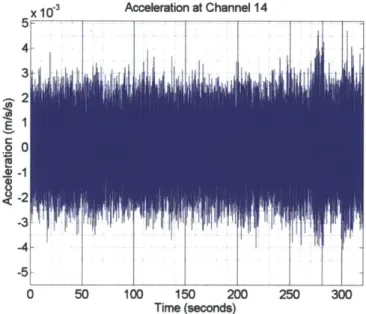
Few physical systems are completely stationary, especially on large time-scales. However, for civil structures with data sampling over durations of minutes, stationarity and ergodicity are generally assumed. Formal tests for stationarity can be carried out, the simplest of which is the Frame Test. In this test, a sampled time history is partitioned into several intervals (or frames), and lower-order statistical moments are computed for each frame. If the statistical moments are invariant with time across the frames, then the process is considered stationary. An example of the Frame Test using Green Building ambient vibrations is presented in Figure 3-1. Here, a 320 second acceleration time-series sampled on June 22, 2012 is partitioned into 4 frames of 80 seconds each. Two lower order moments-the mean and standard deviation-are calculated for each frame. These moments are largely the same across the four frames, indicating that the ambient vibrations can be approximated as being stationary.

(26)

X 10, Accelerabn at %Wonr a

I

.1

I'M""'

I..

I-Acceleration time series collected using the Green Building accelerometer array are considered to be either stochastic or superimposed stochastic-deterministic processes-corresponding to ambient vibrations and strong-source events, respectively. As mentioned above, and demonstrated in Figure 3-1, Green Building motions are assumed to be stationary and ergodic. It follows that spectral and statistical methods, namely Fourier analysis, covariance, correlation, power spectral densities, and coherence should be used in the analysis of Green Building vibrations. These methods are explored in greater detail below.

3.2 Fourier Analysis

Fourier analysis is a principal method for depicting a signal in the frequency domain, and it is a key component in the estimators for some of the statistical analysis methods described later in the chapter. A brief overview of the Fourier analysis, series, and transform is presented here. The cornerstone of Fourier analysis is the assumption (largely true) that a signal can be accurately represented by a superposition of appropriate sines and cosines. The relative contribution of these sinusoidal terms is representative of the energy distribution as a function of frequency, found in the original time series. Fourier analysis can be applied to either continuous or discrete signals, which in turn can be either

507 ₁₀₀

(27)

periodic or aperiodic. For continuous periodic signals, the analysis is performed by expanding the time history into the Fourier series, where the signal is represented by sinusoids of discrete frequencies, corresponding to the fundamental frequency, w1 and its harmonics (integer multiples of wi). The Fourier series decomposition of a signal x(t) with a period T is shown in Equation (3.1), with the formulas for the coefficients An and Bn provided in Equations (3.2) and (3.3). It is often convenient to express the Fourier decomposition in complex notation with a single coefficient, C. (Equations (3.4) and (3.5)). The magnitude of the coefficient C, indicates how a signal's power is distributed across different frequencies. Another quantity emerging from the Fourier coefficients is the phase angle (Equation (3.6)).

00

x(t) = 0.5A0 + Z(An cos(Wkt) + Bfsin(Okt) (3.1)

i=1 An = fx(t) cosSont) dt n = 0,1,2,... (3.2) T 0 Bn = fx(t) sin(On t) dt n = 0,1,2, ... (3.3) T 0 x(t) = Cewnt (3.4) n=-00 C= 0.5(An -jBn)= f x(t)e-j"ntdt n = ±(1,2,3,...) T 0 (3.5) Co = 0.5A0 On = tan-1 B (3.6) An

The principle of Fourier series can be extended to the case of discrete, aperiodic signals-such as those encountered in the Green Building acceleration data-by introducing the Discrete Fourier Transform (DFT). The basic formula for the DFT is found in Equation (3.7). In this equation, x(t) is a signal in the time domain sampled at a time interval of At with a total of N samples, x= x(nAt), and X is

the resulting Fourier spectra. The time-domain signal can be recovered by applying the same formula to

its frequency-domain representation (Equation (3.8)). The specific variety of DFT used was the Fast Fourier Transform (FFT) algorithm, as implemented in MATLAB. Fourier analysis will be applied to the

(28)

Green Building accelerometer data to identify the structural periodicities, calculate the power spectra (Section 3.5), and to perform frequency domain averaging (Section 4.1).

N-1 Xk = xne 2jkn/N k = 0,1,2, ... N - 1 (3.7) n=O N-1 xn= Xke 2jnkn/N n = 0,1,2, ... N - 1 (3.8) k=O

3.3 Covariance

The covariance is a statistical measure which quantifies how two signals change with one another. Specifically, covariance tracks the linear dependence of two random variables. The covariance function compares the signals as a function of a time lag z between them. The lag variable can also represent other quantities besides time, such as spatial separation. For random variables x(t) and y(t) with sample size N, the covariance and the cross-covariance functions are computed using Equations (3.9) and (3.10). A positive covariance indicates the signals are changing together in the same direction, a negative covariance indicates that they are changing together but in opposite directions, while a covariance of zero means that the signals have no common trends. In the special case where the two signals are the same (x(t) = y(t)), the covariance reduces to the variance of the signal, given by Equation (3.11). The magnitude of the covariance does not have a meaningful physical interpretation. Thus, it is difficult to establish what the strength of the relationship between two signals is, and it makes comparison of different signal pairings impossible. The covariance will primarily be used to compute the correlation function, which is described in the next section.

N

Cov(x, y) = oxy = E[x - E(x)] * E[y - E(y)] = (x - )(y₁- (3.9)

N--T

Cxy(T) = E[x(t) - E(x)] * E[y(t + r) - E(y)] = (xt - )(Yt+x - )(3.10)

N - T t=1 N Cov(x) = ox 2 ₌ _E[x 2] - E (x)2 = x Xi2x _ 2 (3.11) i=1

(29)

3.4 Correlation

Correlation, like covariance, is a statistical measure which estimates the linear dependence between two signals as a function of the time shift (T) between them. As with covariance, T can also represent shifts in other quantities, such as spatial position. Two correlation values are of interest-the correlation function and the correlation coefficient function (sometimes known as the Pearson product-moment correlation coefficient), which will henceforth be referred to as the correlation coefficient. The correlation function is defined in Equation (3.12). The correlation coefficient function is found by dividing the cross-covariance function of two signals by the product of their standard deviations. For random variables x(t) and y(t) with sample size N, the correlation coefficient is given by Equation (3.13). A special case of the cross-correlation is the auto-correlation, in which the signal is compared to itself. In this case, Equation (3.13) reduces to Equation (3.14). Dividing by the standard deviation normalizes the covariance, and gives a correlation coefficient on the range of -1 to 1. This gives information on the strength of the linear relationship between the signals and makes it possible to compare different signal pairs. Signals with correlation values of +1 have a strong linear relationship (changing together in the same or opposite direction), while those with correlations of 0 are completely random or have a perfectly non-linear relationship. A common rule of thumb holds that correlations of 0.7 to 1.0 are strongly correlation, values between 0.3 and 0.7 are moderately correlated, and values between 0 and 0.3 are weakly correlated and can be considered random. These conventions are summarized in Table 3-2.

In the context of the Green Building accelerometer data, correlations will be used to estimate the degree to which energy propagates between successive floors and to compute the power spectral density function. Applied to spatial lags, the correlations will be used to find the area of effect of certain sources and to compare the behavior of the east and west sides of the building.

N-r

Rxy

(r) = E[x(t)y(t + T)] = N (xi(yi+r) (3.12)

t=1

CXYQ) N -T Tt= (Xt - x)(Yt+1

-Pxy () - X Y _-UXU

where _(3.13)

N

=X = E[x2] - E(x)2 (Xi2 _ 2

(30)

Cxx(T) N - t = (xt -)(X+T- (3.14)

pU() = 2 2

Table 3-2: Rules of thumb for interpreting correlation values

Correlation Value Nature of Dependence

0.7 to 1.0 (or -0.7 to -1.0) Strong

0.3 to 0.7 (or -0.3 to -0.7) Moderate

0 to 0.3 Weak or Random

3.5 Power Spectral Density

The power spectral density (PSD) is a frequency decomposition of a random process. It is estimated by taking the FFT of the correlation function. Like correlation, the PSD can be computed for two different time series (cross-PSD) and for the same signal (Auto-PSD), as shown in Equations (3.15) and (3.16). Conversely, the correlation function can be recovered, by taking the inverse FFT of the PSD. The PSD may also be computed by taking the FFT of the input time series directly. This approach is often computationally and conceptually simpler, and Welch's Method (a type of FFT-based PSD estimator) is the most commonly used method to compute the PSD. Welch's method is omitted here, but the standard procedure for FFT-based PSD estimation is summarized below. Given two random processes, x(t) and y(t), a set of N time histories may be collected. For a time history n, the FFTs of the variables are given by Xn(t) and Yn(t). The PSDs may be computed by multiplying Yk(t) with the complex conjugate of Xk(t)

and averaging over the N collected sample histories, as shown in Equations (3.17) and (3.18). Due to the double-sided integral in the Fourier transform, the PSD has mirrored positive and negative frequencies. To ease physical interpretation, the one-sided cross-PSDs and auto-PSDs-denoted as G in Equations (3.19) and (3.20)-are often used in signal analysis.

+00

Sxy (w) = FFT

(

Rxy )) =f Rx, (r) e1-0 T dT (3.15)

(31)

N

S )= E(X*(w)Y(w)) = N Xi*() Yi(0) (3.17) i=1

N

Sxx(a)

=

E(IXn(w)|

2

)

= IXi(O)|2 (3.18)

i=1

GXY (o) = 2S() a > 0 (3.19)

SXy(w) o = 0

Gxx(o) = 2SXX(a) W > 0 (3.20)

SXX() o = 0

The PSD amplitude for some time-history, y(t), has units of [y(t)]2

/Hz. In the case of acceleration time histories, this comes out to be (m/s2

)2/Hz. The auto-PSD can be thought of as representing the average power carried by the time series as a function of frequency, and the area beneath the PSD curve in a selected frequency band is the squared RMS value for that band. To ease interpretation, the PSD can be integrated as in Equation (3.21), to yield the cumulated spectrum power (CSP). This gives a better idea of the relative contributions of particular frequencies. Unlike the auto-PSD, the cross-PSD is usually complex valued. The real and imaginary components of the PSD are called the coincident spectral density function (or cospectrum) and quadrature spectral density function (or quadspectrum). The magnitude and phase angle spectrum of the PSD can be computed by decomposing the PSD into its real and imaginary components (Cxy and

Qxy)

and applying the standard equations. The amplitude spectrum measures how relative signal power varies between the two signals as a function of frequency, while the phase spectrum indicates frequency phase shift.

CSP(0j)

f

Gxy (a) dw (3.21)

0

Another useful application of the PSD is in mode-shape estimation. Assuming that natural frequencies have been determined and that there are a sufficient number of sampling locations on a structure, the approximate mode shape of the structure can be found using Equation (3.22), where cpn is the mode shape of the nth natural frequency (fn) at location m, and Xm(t) is a time history sampled at

(32)

locations should be distributed evenly throughout the structure. To estimate the shape of a mode p, time histories from about p locations will be required. This relation is best used only for small modal damping ratios, generally about ( < 0.05. For the Green Building dynamic characterization, the PSD will be used to compute signal coherence (covered in the next section), to identify periodicities in structural motions, and to determine approximate mode shapes.

<pn(Xm (t) = Gxmxm(fn) (3.22)

3.6 Coherence

The coherence function, sometimes called the magnitude squared coherence, is a normalized measure of the correlation of two signals in the frequency domain. It conveys similar information as phase angles, but it is visually easier to interpret. The coherence spectrum is computed using the signal PSD's and Equation (3.23), below. It is often useful to compute the square-root of the coherence function, Equation (3.24), to determine the sign of the linear relationship of the signals. The coherence values follow the same rule-of-thumb as correlation (Table 3-2), with values of +1 signifying the signals to be changing together (either positively or negatively) and 0 indicating a completely random relationship between the two. The coherence function is useful for estimating the effect of noise on a system, and it will be applied to the Green Building for natural frequency identification and mode shape estimation by assessing how different parts of the structure move with one another as a function of frequency.

|Gxy

(f )|z

yxy2 f) = G (f) (3.23)

Gxy (f)|

yX,(f)

= G (f) f (3.24)

Gxx (f) Gyy (f )

3.7 Visual Colormap Analysis

To better recognize structural behavior and identify modal characteristics, it is often helpful to examine the signal set holistically, as opposed to by individual time-history. A convenient and conventional tool for this purpose is the colormap-a visual representation of a system where a color-scale is used to represent the value of some quantity of interest. In this case, the system is the Green Building as represented by 36 accelerometers, and the quantities of interest are accelerations,

(33)

The colormaps were created as two-dimensional images using MATLAB. First, a blank synthetic image was created with the same aspect ratio as a desired fagade of the Green Building. Next, the appropriate sensor time-histories were associated with points on this image, corresponding to the actual accelerometer locations in the building. The motions at the remaining points were found by assuming a linear interpolation between the defined accelerometer locations-first in the vertical and then in the horizontal direction. A color-scale was then applied to the image, based on the extreme motion values. For extra flare, the colormap was made slightly transparent and superimposed on a photograph of the Green Building. An example of a single colormap from the 10/16 Hollis Center earthquake is pictured in Figure 3-2. This process was repeated for each time point, and the resulting images were then collected into a movie.

These colormap animations are useful since they allow motions to be seen and interpreted throughout the structure and as an evolving function of time. Using them, it is possible to view the characteristics of energy propagation through a structure and to estimate the locations of excitation sources. More importantly, they can be used to estimate mode shapes and verify the identity of modal frequencies. This is performed by applying a band-pass filter to the full data set around some frequency band of interest, per the filtering methods described in Section 4.2 below. The visualization is then run on the filtered data set, and the resulting motions describe the structural response due to the selected frequency. If the selected frequency is a normal mode of vibration, the visualized motion is the corresponding mode shape. This method was used to check the motions associated with the identified natural frequencies and to estimate the location of nodal points in mode shapes.

Accleration (m/s/s) at: 31.45 seconds

0.06 0.036

-0.012

0

Figure 3-2: Colormap plot of Green Building accelerations in the NS direction due to the 10/16 Hollis Center Earthquake

(34)

4 Data Pre-Processing

For analysis of the Green Building data and similar data sets, the methods outlined in the preceding section can be applied to the collected data. It is also often desirable to integrate or differentiate the data to get a full set of displacement, velocity, and acceleration responses. However, real systems and instrumentation often admit features into recorded data which make direct integration and application of these analysis methods error-prone. One problem is that of signal noise-either electronic or stemming from ambient vibrations-which can mask features of interest in the time-domain and implant spurious frequencies in the frequency domain. Significant problems also arise from DC errors occurring in electronic sensing systems and low-frequency variations in either the sensors or the structural system under study. Both features complicate time-domain integration and analysis done in the frequency domain. Due to these errors, collected time histories must usually undergo some pre-processing to eliminate the corrupting features. Three pre-processing methods used for the Green Building data are summarized in this Chapter. Section 4.1 covers frequency domain averaging, filtering is reviewed in Section 4.2, and a summary of base-lining is presented in Section 4.3. To demonstrate the necessity of these methods, Figure 4-1 shows a comparison between minimally processed displacements and those which have been filtered and base-lined. Both time histories from the same ambient signal, and they were integrated from accelerations using the trapezoidal method.

x 104 Displacement at Channel 20 (Minimally Processed) x 10- Displacement at Channel 20

1

3-0.5 2 EE

I

0 -1.5 0 50 100 150 200 250 300 0 50 100 150 200 250 300

Time (seconds) Time (seconds)

Figure 4-1: Comparison of displacement time histories from a minimally processed signal (left) and from a filtered and base-lined signal (right)