Design of a free-running, 1/30th Froude scaled model destroyer for in-situ hydrodynamic flow visualization

Design of a Free-running, 1/30th Froude Scaled Model Destroyer for

In-situ Hydrodynamic Flow Visualization

By

David M. Cope, LT USN

United States Naval Academy, 2007

MASS~AdHUSETTS INSTI UTE

OF TECHNOLOGY

JUN28 2012

LIBRARIES

ARCHVES

Submitted to the Department of Mechanical Engineering In partial fulfillment of the requirements for the degrees of

Naval Engineer and

Master of Science in Mechanical Engineering at the

MASSACHUSETTS INSTITUTE OF TECHNOLOGY

June 2012

0 2012 Massachusetts Institute of Technology. All rights reserved.

Signature of Author...

N

7a

Naval Construction and

A i / f

MIT Sea Grant Engineering Program (Course 2N) May 11, 2012

Certified by...

f

Doherty Professor of Ocean Science and Engineering Director, MIT Sea Grant College Program

f

Professor David E. Hardt Chairman, Departmental Committee on Graduate Students

/I

Design of a Free-running, 1/30th Froude Scaled Model Destroyer for

In-situ Hydrodynamic Flow Visualization

By

David M. Cope, LT USN

Submitted to the Department of Mechanical Engineering

On May 11, 2012, in Partial Fulfillment of the Requirements for the Degrees of Naval Engineer

and

Master of Science in Mechanical Engineering

ABSTRACT

Hydrodynamic flow visualization techniques of scaled hull forms and propellers are typically limited to isolating certain operating conditions in a tow tank, circulation tunnel, or large maneuvering basin. Although cost effective, these tests provide a limited perspective on the interactions of the entire system. Full-scale testing, other the other hand, provides real world data but is costly. In between, a Froude scaled, free-running model of an existing hull form controls costs but also provides superior hydrodynamic data that can be translated more accurately to full scale. This thesis details the design and construction of a 1/3 0th scale free-running model of the David Taylor Model Basin 5415 hull, the precursor to the ubiquitous Arleigh Burke Guided Missile Destroyer hull. The model serves as an experimental platform for advanced maneuvering and propeller crashback studies.

The propeller crashback (a core propulsion plant test for both the U.S. Navy and commercial vessels) imparts significant unsteady loads to the engineering plant and drive train. Each of these is respectively of interest to propeller designers and the Electric Ship Research and Development Consortium (ESRDC). The 1/3 0th scale model provides unsteady, time-resolved, accurate 3D flow visualization and propeller loading data as well as measurements of the effects on the electrical propulsion motors. Testing conducted with the model provides the real world effects of the propeller flow interaction with the hull and appendages.

The second area of research concerns the high inefficiencies of slender hull forms while maneuvering. During a turn, a significant amount of power is lost to the low pressure region

developed on the inside of the turn from shedding vortices that originate along the keel. This increases the tactical diameter of the turn and reduces the turning efficiency of the vessel. Research is currently being conducted around controlling the shedding of vortices and keeping them attached to the hull thereby increasing the turning efficiency and decreasing the turning radius of the vessel. The final area of interest is in forward mounted podded propulsors for use on large vessels.

Thesis Supervisor: Chryssostomos Chryssostomidis

Title: Doherty Professor of Ocean Science and Engineering Director, MIT Sea Grant College Program

ACKNOWLEDGEMENTS

Although it may appear that the design and construction of this model was the work of one person, nothing could be further from the truth. I am in great debt to a number of persons in academia, industry and the Navy. First and foremost, Professor Chryssostomos Chryssostomidis who provided the initial design concept and funded the construction of the model. Dr. Brenden Epps' patience, expertise, and mentoring in no small part kept the project on track and moving forward. Mike Soroka's vast knowledge of all things engineering and fabrication as well as his dedication to the project was an invaluable asset. Mark Belanger of the Edgerton Student Shop taught me the machining skills necessary to construct several components of the model. The engineers at Marine Applied Physics Corporation, Paul Dillingham and Kyle Moseson, who took my initial design and built a spectacular model and handled the design alterations with ease, are much appreciated. Mark Lamattina and Craig Deady, respectively of Target Electronic Supply and Kaman, lent me their time and knowledge on countless occasions to get the model control system and motors operating. When the size of the model grew too large to manage at Sea Grant's MIT lab, we went into a scramble trying to locate a lab space to house the model and complete the assembly. Fortunately, the generous people at Bluefin Robotics (Quincy, MA) again reaffirmed the close relationship between themselves and MIT Sea Grant and provided a first class facility to complete the project. Specifically, Will O'Halloran and Harvey Duplantis provided unyielding support at a moment's notice, without which the project would not have reached its current state.

Table of Contents

Abstract ... 3

A cknow ledgem ents... 5

1 Introduction... 9

1.1 Background and Overview ... 9

1.1.1 The Crashback Maneuver and Current Extent of Research... 9

1.1.2 3D Synthetic Aperture Im aging for Fluid Flow s ... 16

1.1.3 Free-running M odel Testing ... 18

1.2 Project Goals... 21

2 M odel Design ... 21

2.1 DTM B 5415 ... 21

2.1.1 Hull Background... 21

2.1.1 Scaled Hull Specifics... 22

2.2 M odel D esign and Construction Process ... 24

2.2.1 General M odel Design ... 24

2.2.2 Propulsion ... 26

2.2.3 M aneuvering... 33

2.2.4 Pow ering... 39

2.2.5 Control... 46

2.2.6 Onboard Sensors... 47

2.3 Perform ance Characteristics... 48

2.3.1 Open W ater Trials... 48

2.3.2 Testing Conditions Specific to Future Research... 48

3 Future Experim ental testing ... 50

3.1 Crashback Transients ... 50

3.2 Increasing slender body turning efficiency ... 51

4 Conlcusions... 52

4.1 Future W ork and Lessons Learned... 52

W orks Cited ... 53

5 Appendices... 55

Appendix C-IMS MDrive23 Stepper Setup Code ... 57

Appendix D-Balder e100 Control Code for MINT Workbench... 58

Appendix E-Ship Construction Specification to Maritime Applied Physics... 69

Appendix F-Internal Equipment General Arrangement ... 72

Appendix G-Model Controller and Motor Wiring... 73

A ppendix H -M odel W eight Report ... 74

A ppendix I-B ill of M aterials... 76

List of Figures

Figure 2-Time averaged axial velocity streamlines from LDV at J=-0.7 (Reproduced from [2]) 10 Figure 3-Sectional blade inflow vectors ... I 1 Figure 4-Crashback instanteous inflow and time averaged inflow... 12

Figure 5-Crashback inflow velocity comparison(Reproduced from [2]) ... 12

Figure 6-Time averaged and instantaneous propeller disk flow during crashback (Reproduced fro m [3 ])... 13

Figure 7-Thrust power spectral density, experimental in blue, LES simulation in red (Reproduced fro m [5 ])... 15

Figure 8-Side force power spectral density, experimental in blue, LES simulation in red R eproduced from [5]) ... 15

Figure 9-Synthetic aperture example (Reproduced from [9])... 18

Figure 10-Hughes and Allan turbulent stimulation method (Reproduced from [11])... 19

Figure 11-David Taylor Model Basin 5415 lines ... 21

Figure 12-Initial design with three flow visualization windows ... 24

Figure 13-Stern w indow location... 25

Figure 14-Initial stern w indow view port ... 25

Figure 15-Notional internal equipment layout... 25

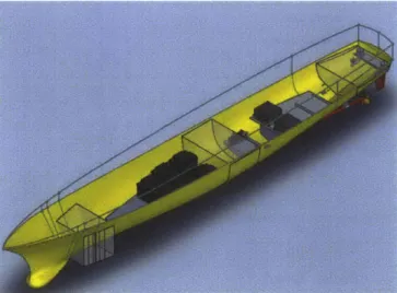
Figure 16-Isometric view of model as built... 26

Figure 17-DTMB 4876 and 4877 propellers on DTMB 5415 model (Reproduced from[19]) .... 27

Figure 18-Contours of axial velocity, x/l = 0.9603, nominal wake (Reproduced from [19])... 27

Figure 19-Contours of axial velocity, x/l=0.9603, propelled (Reproduced from[19])... 28

Figure 20-Modified blade thickness profile and Solidworks rendering of propeller 4381... 30

Figure 21-Full four quadrant data for propeller 4381... 31

Figure 22-Off-design propeller speed analysis. Note same data as Fig 17, Quadrant 1 (0<p<90) ... 3 2 Figure 23-Required propeller RPM and delivered thrust ... 33

Figure 24-DTMB 5415 stern arrangement as designed (Reproduced from [18]) ... 35

Figure 25-Final strut configuration... 36

Figure 26-Ship and rudder orientation during a steady turn ... 36

Figure 27-Model stable turning radius versus rudder angle at full scale speed of 20 knots... 39

Figure 28-Full scale DTMB 5415 effective resistance comparison ... 40

Figure 29-Blade element (Reproduced from[23]) ... 44

Figure 30-Vortical flows around the DTMB 5415 hull in steady maneuver at a static drift angle = 100 (left) and Steady turn (right) (REproduced from [17]) ... 51

List of Tables

Table 1-DTMB 5415 full scale particulars[18] ... 23

Table 2-Relative blade stiffness at 0.72 blade radius ... 31

Table 3-Required propeller RPM at selected speeds ... 33

Table 4-Rudder design characteristics ... 35

Table 5-Model propeller inertia ... 45

1 INTRODUCTION

1.1 Background and Overview

1.1.1 The Crashback Maneuver and Current Extent of Research

Large commercial and naval vessels alike constantly operate in congested sea lanes both on the open ocean and along the land-sea interface. In extreme circumstances, it is necessary to bring these several thousand ton vessels to an immediate stop to avoid collision or grounding. To achieve this maneuver, deck officers execute what is called the crashback maneuver, throwing the propulsion train into full reverse while operating at high ahead speeds. From the propeller's point of view, this maneuver is characterized by the forward inflow from the ahead motion of the ship while the propeller operates in reverse. If outfitted with a fixed pitch propeller, the entire drive train must decelerate to zero speed and accelerate in the astern

direction, making the propeller's designed trailing edge the new leading edge. With controllable pitch propellers, the drive train maintains its ahead speed and the blades of the propeller

mechanically rotate their pitch angle at the hub, effectively changing the inflow angle and reversing the direction of thrust. In both instances, the severity of the maneuver imparts extreme loads on both the propeller and drive train and has led to blade failure and damage to the

shafting, reduction gears and main engines. The interaction of the opposing flows and resulting unsteadiness makes the crashback condition particularly difficult to analyze. Figure 1 depicts the dominant flow streamlines during the crashback event.

Reverse _{Recirculating flow}

Thrust(

Because of the potential for failure, the U.S. Navy includes this extreme off-design condition as a standard test of the engineering plant during delivery of a new ship and regularly throughout the life of the ship. Most of the propellers in the Navy's inventory are highly skewed and are more susceptible to blade failure from extreme loading. The leading ship engineering and research arm of the Navy, Naval Surface Warfare Division Carderock (NSWC-CD), has conducted extensive testing and research around the maneuver at both model and full scale. The core of the research has been conducted in recirculating water tunnels measuring blade stress and imaging the flow around the propeller through particle image velocimetry (PIV) or laser doppler velocimetry (LDV). Jessup et al. (2008) conducted a thorough examination of flow velocities around propeller 4381 at two advance coefficients, J=-0.5 and -0.7, in NSWC-CD's 36 inch water tunnel. The imaging was done in the X-R plane. Time averaged results show the distinctive vortex ring around the blade tip, caused by the downstream (astern) flow from the moving ship and the reverse flow through the propeller disk. As would be expected, the vortex ring shifts aft and expands as the free stream velocity increases (more negative J). Figure 2 shows the time averaged vortex ring around the blade tip.

101 ₂

x

FIGURE 2-TIME AVERAGED AXIAL VELOCITY STREAMLINES FROM LDV AT J=-0.7 (REPRODUCED FROM [2])

Also witnessed during the course of the research was a diffuse blade wake which Jessup (2008)' attributed to the unsteadiness of the blade flow during crashback event. This time-averaged velocity data was then utilized to calculate the mean blade stresses on each blade using

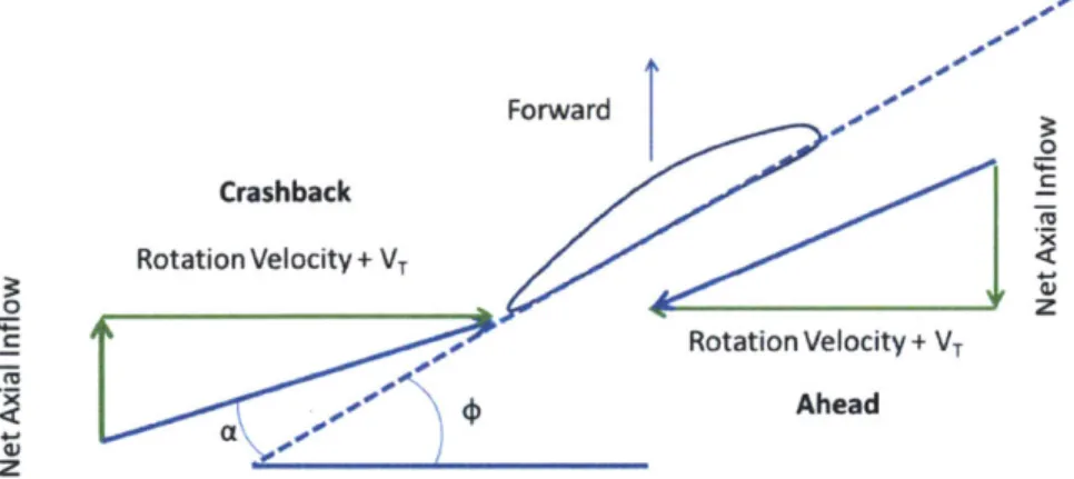
trailing edge because of flow separation. Jessup (2004) also notes that the standard geometric angle of attack when considering the 2D flow diagrams does not accurately represent the actual inflow and over predicts the angles of attack. As is seen in Figure 3, the net axial inflow to the blade sections is governed by the suction of the propeller and not the astern flow from the ship [2]. Figure 3shows the blade section inflow vectors where a is the angle of attack and <D is the local pitch angle.

Forward Crashback Rotation Velocity + VT 0 z Rotation Velocity + VT Ahead z

FIGURE 3-SECTIONAL BLADE INFLOW VECTORS

Of more interest than the average flow is fully time-resolved flow because of the large

amount of unsteadiness around the propeller during crashback. The unsteadiness is seen in the sporadic inboard and outboard movement of the vortex ring and causes large fluctuations in thrust and torque on the propeller and drive train. PIV shows that the vortex moves from a time averaged location of 1.7 radii outboard to well inboard of the blade tip. The NSWC-CD research found that when the ring vortex moves inboard, towards the hub, the local axial flow at the blade tip is reversed from the time averaged axial flow. This drastically shifts the local angle of attack and was hypothesized to cause the extreme blade loads recorded by strain measurements along the root. Figure 4 compares the averaged axial inflow with the instantaneous reversal of the

inflow caused by the oscillating ring vortex and Figure 5 shows Jessup's (2004) measurements of the flow's average velocity compared with velocities during an extreme blade loading event.

Forward

Instantaneous

Va

Time Averaged

FIGURE 4-CRASHBACK INSTANTEOUS INFLOW AND TIME AVERAGED INFLOW

Images of blade cavitation showed shifting, unsteady patterns along the leading edge of the blade. The irregular cavities were attributed to the stall that occurs when the local tip flow reverses as discussed above. These low pressure cavities add to the extreme, instantaneous blade loading. A blade element approach using solely the extreme axial velocities found that blade thrust was 215% and torque was 188% of the mean crashback state. The root bending moment was 280% greater than the mean due to the excessive tip loading [2].

1. 0. 0. o. n. FIGURE 5-CRASHBACK 20 60 - - -- -- - --- --- -I | 0 --- -- - ----15 1 05 0 0.5 1 11

INFLOW VELOCITY COMPARISON (REPRODUCED FROM [2])

NSWC-CD crashback research also analyzed the side forces imparted on the propeller.

The primary focus of the effort was to map the asymmetrical behavior of the ring vortex around the propeller disk. Whereas earlier investigations took PIV data from the X-Z plane, the authors now focused on imaging the Y-Z plane to capture the instantaneous unsteady flow over the entire

the side force on the blades and hub. Using shaft dynamometry and tri-axial strain gages on the blade, Jessup et al. (2006) tested at advance coefficients from -0.3 to -1.0. Their findings included strain peaks as high as 3.6 times the average. They confirmed that the region from -0.5 to -0.75 has the greatest amount of unsteadiness, as witnessed in earlier trials. Analysis of the

side forces found that they maintain 7-8% magnitude of the average thrust through time. Time-averaged Stereo PIV (SPIV) images of the propeller disk showed a symmetric inward radial flow across the face of the propeller. However, a series of instantaneous images over a three second time period revealed predominantly unsteady, asymmetric flow. Samples of these images are

shown below in Figure 6. A longer series of the images shows the flow field rotating around the shaft axis.

FIGURE 6-TIME AVERAGED AND INSTANTANEOUS PROPELLER DISK FLOW DURING CRASHBACK

(REPRODUCED FROM [3])

Adequate computational modeling of the crashback maneuver has been limited because of the large amount of unsteadiness around the propeller disk. Propellers operating in normal ahead or backing conditions are well documented through Reynolds-Averaged Navier-Stokes

(RANS) modeling and potential flow models [4]. However, when applied to the highly unsteady

flow conditions during crashback, these methods fail to agree with experimental data. Chen & Stern (1999) applied RANS to all four flows around a DTMB 4381 propeller (ahead, backing, crashahead, crashback). While they found good agreement with ahead and backing flows with differences of 5% and 6.5% for thrust and torque predictions respectively, the predictions for the

highly turbulent crashahead and crashback flows were 110% different from experimental values. RANS also failed to capture the high amplitude oscillations around the mean thrust and torque

Noting the failure of RANS modeling in analyzing propeller crash flows, Mahesh and Vysohlid (2007) applied large eddy simulations (LES) to the problem because of its inherent ability to capture large scale turbulence. Modeling the computational domain and propeller to match that of Jessup's (2004) water tunnel experiments, Mahesh and Vysohlid (2007) simulated crashback conditions over 300 propeller revolutions in order gather more reliable statistics and derive power spectral densities of thrust, torque, side-forces and cross flow. All simulations were run at an advance ratio of J= -0.7 and a Reynolds number of Re = 480,000 defined as

U DU

1=-

Re=-Dn' v

Where U is the free-stream velocity, n is the propeller rotational speed in revolutions per time unit, D is the propeller diameter and v is the kinematic viscosity. The calculated thrust and torque revealed large amplitude, low-frequency oscillations, comparing well with Jessup's experiments. Plots of the power spectral densities (PSD) of the simulated and experimental thrust and side force showed good correlation around the frequency of 5 rev-' for thrust and torque. This corresponds to motion of each blade of the five bladed propeller. The lobes and greater spectral density in the experimental values, especially at the higher frequencies, were attributed to blade bending, blade vibration and other resonances of the experimental shafting and machinery [5].

10--8 10 Q- 106 10 10 10~ 100 10 frequency [rev-1

FIGURE 7-THRUST POWER SPECTRAL DENSITY, EXPERIMENTAL IN BLUE, LES SIMULATION IN RED

(REPRODUCED FROM [5]) 101 2d Vg II ii 1 1 - - M 10 10 10 10 frequency [rev~1I

FIGURE 8-SIDE FORCE POWER SPECTRAL DENSITY, EXPERIMENTAL IN BLUE, LES SIMULATION IN

RED REPRODUCED FROM [5])

Mahesh's and Vysohlid's (2007) subjective comparison of Jessup's (2006) experimental PIV data and the LES simulations revealed differences in the manifestation of the ring vortex during crashback. While the axial velocities showed good agreement, the ring vortex was closer to the propeller in the simulation than it was in Jessup's experiments. Axial, radial, and

exception at the blade tip, where the experimental values showed a much larger RMS fluctuation than was simulated.

The loads during crashback are largely due to the unsteady ring vortex that oscillates upstream and downstream and rotates around the propeller disk plane. A primary difference between the normal ahead operation and the crashback condition is the sign of the pressure differential across the blade face. Whereas in the ahead condition, the high pressure,

downstream blade face is pushing the blade in the opposite direction of the free steam, in the crashback condition, the pressure side pushes the blade in the same direction as the free stream

[5]. While Mahesh and Vysohlid (2007) validated the use of LES simulations in modeling the

crashback condition at steady advance coefficients, further simulation could examine the unsteady load effects during an actual crashback and a dynamic advance coefficient. Prior research on flapping-foil propulsion has revealed that the load effects of unsteady stall and leading edge separation induced by dynamically changing the angle of attack are not trivial [6].

1.1.2 3D Synthetic Aperture Imaging for Fluid Flows

Accurate measurement of fluid flow characteristics around the hull of a ship provides engineers with data to better design the propellers. To ensure the accuracy of the measurements, non-intrusive flow visualization techniques such as LDV and PIV are applied. These methods are used heavily in characterizing propeller and hydrofoil flows in a stationary setup. PIV requires that the fluid be seeded with small particles that trace the flow path. The fluid volume or plane of interest is illuminated, typically with either a laser or a strobe, and high speed cameras capture the motion of the seed particles. Using post processing software, the speed and direction of the particles can be derived. Until the last decade, all PIV was conducted in a stationary manner, where the plane of interest and the body remained fixed in space. To capture the flow field around the hull, the ship model is run past the PIV or LDV setup and an

instantaneous, 2D flow field image is captured. The process of repeated, precisely timed runs at various locations is a difficult and time consuming process. Utilizing an optical imagining

system that traveled with the model would alleviate these complications as well as provide time averaged and instantaneous flow field data. Two recent attempts have been successful in designing and testing moving PIV systems for measuring velocity fields around the hull of a

Cheng Kung University's tow tank [7][8]. The difficulty in building such a system lies in the submergence of the laser for illumination of the field of view and actively seeding the fluid ahead of the model without disturbing the flow. Some of the issues noted by the Taiwanese researchers included image distortion due to air entrained by the bow wave of the ship,

interference of the hull geometry with the desired laser sheet placement, and shadowing of the images caused by the laser reflecting off the model's bright yellow color. Their setup placed the submerged laser astern of the vessel, facing forward and used a camera above the water surface with the field of view provided by a duct and mirrors [8]. The University of Iowa's setup is similar except that it is designed specifically for their facility and would require a significant amount of re-engineering to incorporate the system into another tow tank. All the lasers and cameras of the Iowa setup are fully submerged in the fluid [7].

While the field of 2D flow imaging is mature, 3D imagining is still seeking advancement. According to Belden (2011), the current state of 3D imaging is limited in resolution and

resolvable frame size. A thorough review of three-dimensional flow imaging techniques is discussed by Belden [9]. Additionally, optical occlusions restrict the efficacy of the imaging and, in some instances, the system cannot be extended to multiphase flow problems, such as that of a ship hull, where air has been entrained along the length of the hull due to the bow wave. Belden developed a novel PIV technique incorporating synthetic aperture imaging (SAPIV) to capture 3D fields of view and effectively increase the lens aperture to "see through" partial occlusions. Using an array of several cameras, each captures an image within the field of view, although some parts of the viewport may be occluded. Applying a post processing algorithm that accounts for the depth of the objects due to parallax, the individual images can be refocused on planes within the viewport to reconstruct the 3D space. This method inherently solves the obstruction issue as well as produces a 3D rendering of the event. Figure 9 is a simple schematic explaining the synthetic aperture process taken from Belden's PhD thesis [9]. Belden

successfully developed and validated a 3D SAPIV system with moderately dense fluid seeding (0.0266 ppp) but expected that increasing the seeding for better velocity profile resolution would be practical. The capability of the system is scaled by the number and abilities of the imaging cameras used. The largest volume successfully imaged was 100 x 100 x 100 mm3_{. Imaging of}

the highly dynamic crashback event could greatly benefit from this new flow velocimetry technique. During his validation process, Belden successfully imaged a vortex ring which is

fundamentally similar to the vortex ring that develops around the propeller blades during crashback. The potential future application of Belden's SAPIV method to propeller flow visualization with the present ship model drove the need to design a stern window over the

propellers and rudders of the model that is discussed later. The acrylic window provides a large enough view port and mounting area for an array of up to nine of the Point Grey Research, Inc. Flea2 cameras.

ZI Z

Z2 ZI I 7

Measurement Camera Refocused

Volume Array Images

FIGURE 9-SYNTHETIC APERTURE EXAMPLE (REPRODUCED FROM [9])

1.1.3 Free-running Model Testing

Froude-scaled free-running model tests are typically used within the ship design process to evaluate the maneuvering ability and the course keeping ability of the design prior to full scale production. Though costly, this method continues to be an integral part of the design evaluation process. When equipped with precise position and acceleration sensors, the maneuvering and handling characteristics of the model can be measured and scaled to the full scale ship. The International Towing Tank Conference (ITTC) Recommended Procedures and Guidelines outlines the conditions and practices for all scaled model testing. These include water depth effects, model and full scale similitude, scale effects, and the test and analysis procedures.

Because the model will be operating in open water, whether it is the Charles River or a local rock quarry, the depth to draft ratio will remain above the minimum value of hIT = 4to minimize boundary layer effects [10].

In accordance with the ITTC Recommended Procedures and Guidelines for Ship Models, the bow should be outfitted with turbulence stimulators in the form of studs, wires, or sand grain

strips. Turbulence stimulation ensures that both the model and full scale are in the same flow regime and that the model scale flow is consistent and repeatable across the range of evaluated Froude numbers. As well, the stimulators serve as a method of standardization across all model resistance testing. However, the method outlined in [11] for application of turbulence

stimulators provides a blanket approach to all ship models and does not recognize the relation between stud size and the model's boundary layer thickness. This method, from Hughes and Allan (1951), is summarized in Figure 10.

4

Zf

FIGURE 10-H

8 10 LE N T 4 O Is

L.ENciTH OF' WOFCL (FEET")

oR ANGLES DF ENTRANCE

ELOW 10' STUDS TO BE KEPT

. FAR fOmit AS P0SSBLE

20 22 I% 14 to U 4 fo2b30O 4-0 310 ;s-o _

LEGTW OF MCnEL (METRES)

UGHES AND ALLAN TURBULENT STIMULATION METHOD (REPRODUCED FROM [11])

The overarching function of turbulence stimulation is to rapidly trip turbulence at a controlled location along the length of the ship. On full-scale ships operating at a Reynolds number of 108 or higher, the flow transition will occur at or directly aft of the free stream entry

point on the stem. At model scale, however, the natural laminar-turbulent transition is dependent on several factors including the amount of background turbulence, the model surface roughness and upstream boundary layer profile, the presence of flow unsteadiness, surface temperature, and the local streamwise pressure gradient. The dependence of the transition point on these

conditions is mitigated through the use of turbulence stimulators near the water entry point. As well, the stimulator must be of sufficient size to initiate a rapid transition so that the form drag of the model is not significantly altered. This is quantified in a non-dimensional height ratio, y+, of the stimulator to the local boundary layer thickness. y+ values of at least 300 for

three-dimensional type (e.g. cylindrical stimulators) is required to achieve a rapid transition [12]. Furthermore, the difference between the desired decrease in laminar skin friction drag and the unwanted increase in form drag due to the application of turbulence stimulation devices to the hull should be considered and calculated using the methods provided in [12]. Turbulence

stimulators were not included in the initial design of the model, although it will be operating in a laminar flow condition at a Reynolds number of 9.0 x 106, and should be considered after initial testing and trials.

In addition to the previously mentioned considerations, five conditions must be met in order that the model results accurately represent the full scale handling and maneuvering characteristics as dictated in Principles of Naval Architecture [13].

1. The non-dimensional mass moment of inertia of the model about the z-axis, Iz' should be identical to that of the ship.

2. The model rudder should be deflected to the same maximum angle as the ship rudder at the same non-dimensional deflection rate as that of the ship, i.e.,

,m _ , _ m _sL (2)

'Rmn - 's - M

--3. If the ship heel in maneuvers is to be properly simulated, the Ixx' of the

model as well as its non-dimensional transverse metacentric height must be identical to that of the ship. (In practice, these are difficult conditions to

fulfill.)

4. The model propeller operating slip ratio should be identical to the ship propeller slip ratio. This is particularly important if the rudder is located in the propeller race.

5. If the speed loss in maneuvers is to be properly simulated, the response of

the motor that drives the model propeller to an augment in model resistance should duplicate the response of the power plant of the full-scale ship to a corresponding augment in ship resistance.

Adherence to and deviation from these scaling laws is discussed in Chapter 2. Recommended trial and testing procedures are outlined in [10].

1.2 Project Goals

The primary goal of this project was to design and build a 1/3 0th scale, free-running model of the David Taylor Model Basin hull for hydrodynamic visualization and crashback maneuver testing. Because of the desired scale, the model will be utilized in open water, e.g. the Charles River, Boston Harbor, or a local rock quarry. The model will serve as a flexible test platform for future research within the MIT Ocean Engineering department.

2 MODEL DESIGN 2.1 DTMB 5415

2.1.1 Hull Background

The David Taylor Model Basin 5414 was developed as the preliminary hull form for the

U.S. Navy Aegis guided missile destroyer program in the early 1980's. The hull is characterized by a bulbous SONAR dome on the bow and a transom stem. Propulsion is provided through two

shaft lines. The design speed is defined as 20 knots (33.8 m/s) at full scale. Though no full scale ship has ever been built to the 5415's exact lines, the hull served as the precursor to the DDG 51 Arleigh Burke class of naval vessels that is currently comprised of 61 ships and has set the standard for large naval surface combatants. The lines are shown in Figure 11.

FIGURE 11-DAVID TAYLOR MODEL BASIN 5415 LINES

The hull form has become ubiquitous in naval architecture circles and has been the subject of extensive hydrodynamic testing and validation over the past several decades. Ongoing research

has relied upon the well documented tow tank resistance and planar motion mechanism testing to validate Computational Fluid Dynamics (CFD) codes. The Workshop on Verification and

Validation of Ship Maneuvering Simulation Methods (SIMMAN 2008) is an ongoing effort to validate computational codes with experimentally measured data on several hull forms, including the DTMB 5415[14][15][16][17]. The complex underwater hull geometry lends itself to these validation efforts. The general particulars of the full scale hull and model scale are provided in Table 1.

2.1.1 Scaled Hull Specifics

Aside from the following adjustments, the model hull is a 1/3 0th scaled model of the

DTMB 5415. Early in the design phase, it was decided to omit the bilge keels from the scaled hull form, the primary reason being that they would be highly susceptible to damage during launching operations. Another consideration that had to be made was that the model would be operating in an open water environment where environmental conditions could not be controlled. To mitigate the risk of potentially flooding and swamping the boat, the sheer line was raised to increase the freeboard. Creating a flat surface also allowed for a plexiglass lid that would seal the internal compartments from flooding. The main particulars of the model and full scale DTMB 5415 are shown in Table 1.

TABLE 1-DTMB 5415 FULL SCALE PARTICULARS [18] Scale (A) 1.00 30.0 Main Particulars LWL 466.50 15.6 [ft] BWL 62.50 2.1 [ft] T 20.20 0.67 [ft] Displacement 29,750.90 10.83 [ft3 ] Wetted Surface 31,996.80 36.64 [ft2 ] LCB (%LWL aft of FP) -0.68 -0.68 CB 0.507 0.507 CM 0.821 0.821 Rudders

Type Spade Spade

Wetted Surface 165.80 0.411 [ft2

]

Turn rate 9.0 49.3 [deg/s]

Propellers

Type Fixed Pitch Fixed Pitch

Geometry 4876/4877 Modified 4381

No. of blades 5 5

Diameter 17 6.8 [ft]

Appendages

Bilge keels Yes No

Stabilizing fins No No Test Condition Draft 20.20 0.67 [ft] LCG -2.14 - [ft aft ___________________________MS] GM 6.40 - [ft) ixx/B 0.37 -izz/LBP 0.25 -Design Speed 33.8 6.23 [ft/s] Froude Number 0.28 0.28

2.2 Model Design and Construction Process

2.2.1 General Model Design

The initial design of the model was conducted in Solidworks and included three windows along the length of the hull for flow visualization. The three windows were positioned so as to be directly aft of known locations of vortex generation. Preliminary quotes received from potential model builders showed that inclusion of all three windows would be cost prohibitive and it was decided that only the stem window would be included in the final design. Figure 12

shows the initial design with the three windows along the length of the hull and Figure 13 shows the location of the stem window in relation to the propellers and rudders. The shaft struts were positioned forward of the intended design location to not interfere with the window. However, this was changed in the final design when a method was devised to support the struts in their

originally intended location without interfering with the window. The initial stem window viewport over the propellers and rudders is shown in Figure 14 and the preliminary layout of the

internal electronics and batteries including a notional SAPIV camera array is shown in Figure 15.

As built, the model has four separate compartments separated by three transverse bulkheads. The forward compartment does not hold any internal equipment. The second compartment houses the batteries and power conversion equipment while the third houses the motor controller, the servo motors, and the servo motor drives. The aft most compartment houses the stepper motors and rudder post assemblies. A schematic of the generic internal system configuration is shown in Appendix F.

2.2.2 Propulsion

Design of the propeller for the model presented several issues. To achieve the best possible efficiency, the propeller is designed to a single vessel speed of advance. At that speed of advance, each vessel's wake, and thus propeller velocity inflow, profile is different. The pitch of the blade sections can then be shifted to the ideal angle of attack to provide the most thrust. For the DTMB 5415 model, the wake profile was publically available (Chesnakas and Ratcliffe

2005). In their research, the wake profile of a 1:24.824 scaled DTMB 5415 model at 20 knots

full scale was measured using LDV methods. Testing was conducted both under un-propelled and propelled conditions at several axial locations along the shaft in the vicinity of the propeller. For the propelled condition, the DTMB propellers 4876 and 4877 were used. These are a set of

high skew, opposing direction (left and right handed) propellers designed for the DTMB 5415. Figure 17 is an image of the stem of Chesnakas' and Ratcliffe's (2005) model with the 4876 and

4877 propellers. Figure 18 shows the contours of axial wake velocity at x/L of 0.9603 and

FIGURE 17-DTMB 4876 AND 4877 PROPELLERS ON DTMB 5415 MODEL (REPRODUCED FROM [19]) 0,01 0.26 cs 040 407 *0.06 0062 0O6M 0a06 005

FIGURE 18-CONTOURS OF AXIAL VELOCITY, X/L 0.9603, NOMINAL WAKE (REPRODUCED FROM [19])

401S

4040

4W6

FIGURE 19-CONTOURS OF AXIAL VELOCITY, X/L=0.9603, PROPELLED (REPRODUCED FROM [19])

What can be seen, especially in the nominal wake profile, is the interaction of the strut and shaft wakes. Applying this measured profile to the DTMB 5415 of this project would neglect the importance of this interaction since the struts for the model had to be adjusted from the initial design to accommodate the aft window.

The option of adopting the DTMB 4876 and 4877 propellers that were utilized in Chesnakas and Radcliffe (2005), as well as other DTMB 5415 studies, was considered for the

1:30 model. However, while the geometries were available, no four quadrant flow data was

available. Because one of the primary areas of initial research for the model is the crashback maneuver, not having the full four quadrant data on the propellers would require a separate series of water tunnel tests to measure and document their open water characteristics. Therefore,

propeller 4381, a well-tested and heavily documented propeller, was decided upon as the initial propeller for the model. The DTMB 4381 is a spade type propeller with zero rake and zero skew. To maintain the geometric similarity between the model and full scale, each of the propellers was linearly scaled using the same factor as the hull form, resulting in a diameter of

6.8 inches assuming a full scale DDG 51 propeller diameter of 17 feet. As with all scale model

testing, it is desirable to minimize the ratio of full scale to model scale, although in practice this is hardly achievable. In order to gather accurate thrust and torque measurements of scaled propellers, the propellers must be sufficiently large to mitigate scale effects associated with low

moderately large model scale self-propulsion tests. Principles of Naval Architecture

recommends that because of the aforementioned scale effects, the model scale propeller diameter should be no less than 8 inches and preferably closer to 16 inches. In terms of Reynolds

numbers based on blade chord length at the 0.7 radii, the lowest acceptable figure is 4 x 106. However, if turbulence stimulation is present on the leading edge of the propeller blade, then the propeller operating Reynolds number should be no less than 3 x 105 [20]. The velocity of the blade is calculated as shown in Equation 3.

V = [(0.7wnD)2 _{+ (V)2] 1/2 (3)}

With a geometrically scaled DTMB 4381 propeller diameter of 6.8 inches, the Reynolds number at the design Froude number of 0.28 is 5.38 x 105, below the non-turbulence stimulation

limit but well within the limit set forth by the 1975 ITTC mentioned above for blades with turbulence stimulation. As will be seen below, the method of manufacturing the initial prototype propellers resulted in sufficient roughness along the leading edge to justify application of the lower Reynolds number limit. Another consideration is the previously cited requirement that the propeller slip ratios of the full scale ship and the model be identical. Assuming that the full scale ship would use a propeller geometry similar to the DTMB 4876/4877 with a pitch to diameter ratio (P/D) of 1.549 and a nominal design shaft revolution speed of 100 RPM, the slip ratio, sr, of a full scale DTMB 5415 would be approximately 0.4205. Slip ratio is calculated as

Va (4)

sr =

1-Pn

where P is the pitch of the propeller at the 0.7 radii and n is the propeller rotational speed in revolutions per second. The P/D for the 4381 propellers is 1.21 and the nominal shaft speed at the design speed (Fr = 0.28) is 696 RPM. This results in a propeller slip ratio of 0.3734.

Although the ratios are not identical, the full scale data relies on several assumptions. The model shaft RPM is based on theory and not the actual performance of the system and future iterations of the propellers will have a higher pitch to diameter ratio.

For the initial propeller manufacturing iteration, the cost was significantly reduced by fused deposition modeling (a form of 3D printing) them in ABS-M30 plastic. Previous experience in 3D printing of plastic propeller blades had shown a limiting blade thickness of approximately 0.08 inches for ensuring the trailing edges were printed solid. The blade thickness profile of the DTMB 4381 was adjusted to meet this requirement and the resulting blade

thickness versus radius profile is shown in Figure 20. Changing the thickness profile changes the operating characteristics of the propeller. The effects were thought to be negligible for the first iteration of the design. If required for future experimentation, a more accurate representation of the 4381 should be constructed. Figure 21shows the CT and 1OCq versus

P,

D.2 0.3 0.4 0.5 0.6 0.7 0.3 0.9 1

r/R

FIGURE 20-MODIFIED BLADE THICKNESS PROFILE AND SOLIDWORKS RENDERING OF PROPELLER 4381

Inflw angl Beta

FIGURE 21-FULL FOUR QUADRANT DATA FOR PROPELLER 4381

The water permeability and stiffness of the ABS plastic was addressed by copper-nickel plating the propellers. This technique for producing low cost, accurate and durable model propellers has been utilized by Naval Surface Warfare Center, Carderock Division (NSWC-CR). The same rapid prototyping company used by NSWC-CR, RePliForm Inc., was contracted to plate the two DTMB 4381 model propellers for the project using their proprietary RePliKote technique. The total plating thickness, including both the copper and nickel layers, amounted to

0.004 inches or approximately 102 microns. Table 2shows the relative blade stiffness increase due to plating the propeller blade as well as a solid aluminum blade.

TABLE 2-RELATIVE BLADE STIFFNESS AT 0.72 BLADE RADIUS

Blade Material Young's Modulus (E) 2"d Moment of Area (I) El Relative Stiffness

ABS FDM 1.45 x 10 [psi]' 7.77E-04 [in4] 1.13E+02[lb-in2] 1

Cu+Ni Plated ABS 3.0 x 107 [psi] 8.74E-04 [in4

] 3.01E+03[lb-in2] 27

Solid Aluminum 1.0 x 107 [psi] 7.77E-04 [in4] 7.77E+03[lb-in2

] 69

An off-design analysis of the propeller was conducted to provide a starting point for tuning the propulsion motors during initial open water trials. The thrust coefficient required for the model at each of the off-design speeds was calculated and plotted against the propeller curves. The intersection of the propeller thrust coefficient, KTProp, with the model thrust coefficient,

KTodeI provides the operating advance coefficient, Ioff-design from which the required shaft

RPM can be calculated. The model thrust coefficient was calculated by

1 C1 (5)

KTModel ~ pDz 2 k P(1 - t)(1 - W)z

RTm (6)

c1 =

where RTm is the effective resistance of the model. The thrust and wake factors, t and w

respectively, were assumed constant although in reality these change slightly with ship speed. The intersecting KTModeI and KTProp curves are shown in Figure 22 and the required propeller

RPM versus full scale ship ahead speed is shown in Figure 23.Table 3 shows required propeller speeds at selected model and equivalent ship speeds.

- KT Propeller 4381 0.9 . ... ...- IOKQ Propeller 4381 -Model KT 0. 0. - 02 - .6 0. 0 .3 .. . . . .-.. -.. .-. -. 0 .2 -. . . .. . . . ... -.. . . . ... . . . 0 .1 . . . . ... . . .-.. -. .-.-.-01 0 0.2 0.4 0.6 0 .8 1 Advance Coefficient J

1400 --- Propeller Speed 1200- Propeller Thrust 11200 --z 0 1000-2 800-a 600-400 200 --0 0 5 10 15 20 25 30 35

Equivalent Full Scale Ship Velocity, knots

FIGURE 23-REQUIRED PROPELLER RPM AND DELIVERED THRUST

TABLE 3-REQUIRED PROPELLER RPM AT SELECTED SPEEDS

Fr Vship Vmodel Nmodel

- [kts] [ft/s] [RPM] 0.073 5.32 1.64 185 0.132 9.58 2.95 324 0.205 14.91 4.59 506 0.279 20.23 6.23 696 0.338 24.49 7.55 870 0.411 29.81 9.19 1,164 2.2.3 Maneuvering

Because of the Froude scaling, the full scale Reynolds number of the ship cannot be simulated. The significance of this failure in similitude is witnessed in the maximum lift and stall angles of foils. Froude similitude requires that the model speed be less than the full scale speed, making the Reynolds number for the model rudder much less than the full scale and typically within the laminar flow region. For this project, the Reynolds number of the full scale (Res) DTMB 5415 is 2.2 x 109whereas the model Reynolds number (Rem) is 9.0 x 106 when

operating at a full scale design speed of 20 knots (Fr = 0.28). The effects that have been

identified through wind tunnel testing on standard NACA foils are listed in the Principles of Naval Architecture, Volume III as

1. Maximum lift coefficient increases with Reynolds number because of the delay of stall

angle.

2. Lift curve slope varies little with Reynolds number (also with section shape).

3. Drag coefficient decreases with increase of Reynolds number [13].

Also complicating the matter is the surface roughness effects on maximum lift coefficient.

If operating at very low Reynolds numbers, the flow around the rudder could be laminar.

Laminar flow, being more susceptible to separation, can be the cause of decreasing stall angles in model rudder tests. For Froude scaled models, purely geometric scaling of the rudder will result

in a conservative assessment of the rudder's maximum lift coefficient, and thus the ship's turning ability.

Another scale effect that presents an issue for models equipped with multiple rudders is the difference in the full scale and model scale ratio of propeller race velocity to the free-stream. This ratio is much larger for model scale than full scale and is another Reynolds effect. The ratios differ because the much smaller Rem results in a higher drag coefficient for the model and,

in turn, requires the model propeller to operate at a higher slip ratio than the full scale propeller. As with the other Reynolds number effects, this lends to a conservative assessment of the ships maneuvering abilities [13].

The exact specifications of the DTMB 5415 rudder were not available during the design stage of the project model. The only available information was the extents of the projected shape and the placement along the hull, as shown in Figure 24. The design drawings showed the two rudders canted several degrees outboard.

FIGURE 24-DTMB 5415 STERN ARRANGEMENT AS DESIGNED (REPRODUCED FROM [18])

To simplify the mechanics of the system, the cant was removed and the rudders were placed vertically in the same longitudinal position as the drawings. The rudder sections were constructed using a NACA 0018 foil because it has relatively constant center of pressure and the thickness ratio allows for adequate foil strength while maintaining reasonable drag

characteristics [13]. The aspect ratio, sweep angle and general extents of the foil projected in the centerline plane were maintained from the drawings. The rudders' general characteristics are shown in Table 4.

TABLE 4-RUDDER DESIGN CHARACTERISTICS

II I

NACA 0018

Section Geometry

Sweep Angle 4.6 [deg]

Span 0.518 [ft]

Chord (r/R=0.5) 0.381 [ft] Surface Area 0.411 [ft2_]

Rudder position aft 7.64

of midships [ft]

Effective Aspect _2.74 Ratio

Hoerner Lift Slope

(aCI

Another deviation from the original design was the arrangement of the propeller struts and fairwater. The initial design used Figure 24 as the starting point for the strut placement and angles. However, securing the struts to the aft window proved difficult during construction and required additional structure that obscured the field of view of the window. To mitigate the structural concerns the outboard struts were rotated to be parallel with the center plane of the hull, allowing them to terminate in the hull structure instead of the window. The field of view over the window was preserved by terminating the inboard struts at a longitudinally placed member that was secured to the hull structure forward of the window. This new configuration is shown in Figure 25.

FIGURE 25-FINAL STRUT CONFIGURATION

The estimated steady turning radius of the model was determined using the method outlined in the Principles of Naval Architecture with the orientation shown in Figure 26.

U

Once the vessel in a turn has reached a state of equilibrium, the ship maintains a steady turning radius with v and r having constant, nonzero values andnand t being zero. This is

known as the third phase of the turning maneuver. The linearized equations of motion taken from Principles of Naval Architecture for a steady turn are:

-Yv - (Yr - 'us)r = Y&SR (7)

-Nv - Nrr = NSOR (8)

The linear hydrodynamic derivatives of the DTMB 5415 were taken from the averages of the three research institutions participating in the SIMMAN 2008 workshop. The rudder

derivatives were calculated using Hoerner's method for foils at angles of attack below the stall angle. Because the foil aspect ratio is a strong determinant of performance, the slope of the lift coefficient with respect to angle of attack can be found as shown in Equation 9. This is valid for foils with an aspect ratio greater than 1.

(aCIl

ocl) = 1 1 1

aaa=0 _2nd + - + )

1(AReff) 27r(AReff)

The effective aspect ratio (AReff) is twice the standard aspect ratio because of the reflection

introduced by the hull of the ship.

AReff = 2 -AR = 2 - span ~ 2.72 > 1 (10)

chord

The standard value for d is 0.9. Once Equations 7 and 8 are solved for v and r, and knowing the

control derivatives and stability derivatives, and recognizing that r' = 0 = rL/V and the steady

turning radius R = V/r, then r' = L/R, the turning radius, R, can be found as

R -L [Yv(Nr) - Nv(Yr- ) (11)

In addition to the rudder term, Y5, the lift force of the rudder generates separate hydrodynamic terms that alter the bare hull terms found in the SIMMAN 2008 data. The total lift generated by the rudders is:

YR -L = pARU2(SR +R + V

(12) =YSSR + YRrr + YRvV

where 1

aCl

The resulting hydrodynamic moment on the rudder from the rudder lift force is:

where (16) N = Yxr = NS + NRrr + NRv Ns = Y5xr NRr = YRrXr NRV = YRvXr (17) (18) (19)

Accounting for this correction in the bare coefficients, the steady turning radius versus rudder angle at the full scale design speed of 20 knots is plotted in Figure 27. Note that a negative

rudder angle, as defined in Figure 26, results in a turn to starboard as would be expected of a stable hull form.

120 E co 1000 800 600 400 200 ni -30 -25 -20 -15 -10 -5

Rudder Angle in Degrees

FIGURE 27-MODEL STABLE TURNING RADIUS VERSUS RUDDER ANGLE AT 20 KNOTS

0

FULL SCALE SPEED OF

Using the nondimensional rudder deflection rate scaling requirement discussed above in the modeling, the tandem rudders of the model have to slew at a rate of 0.861 radians per second, or 49.3 degrees per second. Because of the 1:2 stepper motor to rudder sprocket gear ratio, the speed of the stepper motors on the onboard controller were set to twice the deflection rate, or

98.6 degrees per second. Prior to selecting the stepper motors, the approximate holding torque

requirements were calculated using the Harrington method outline in Principles of Naval Architecture, Volume III.

2.2.4 Powering

Typically, when designing the power train of a ship, the designer begins with the towed, or effective, resistance of the hull scaled from model tests in a tow tank. Because of the large scale of the model being built and the lack of facilities available to conduct resistance testing,

|--

data was taken from previous studies on the DTMB 5415 hull form. The studies were from Naval Surface Warfare Center Carderock Division and the University of Iowa's Hydroscience and Engineering College. Each data set was scaled to full scale using Froude's technique and plotted against each other, shown in Figure 28. Equation 20 is Froude's Hypothesis where CD is the total drag coefficient, Cf is the frictional drag coefficient dependent on the Reynolds number, and CR is the residual drag dependent on the Froude number.

CD(Re, Fr) ~ Cf (Re) + CR(Fr) (20)

The INSEAN line is from the University of Iowa, the NSWC-CD line is from a 1984 Navy tow tank analysis and the Tsai line depicts the towed resistance of the full scale DDG 51 hull after changes were made to the initial stem design.

3.50E+03 3.OOE+03 Z 2.50E+03 C m 2.OOE+03 1.50E+03 U 1.00E+03 5.00E+02 0.00E+00 0 0.1 -INSEAN -NSWC-CD -Tsai 0.2 0.3 Froude Number (LWL) 0.4 0.5

FIGURE 28-FULL SCALE DTMB 5415 EFFECTIVE RESISTANCE COMPARISON

The DTMB 5415 test models were at a scale of 1:24.824 and both utilized turbulence

_00Z/

.0

ITTC Ship-Model Correlation Line. Data was taken from "Experiment 33," in which the hull was fully appended, rudders were placed at 0 degrees from the centerline, and no propellers were

installed. The displacement and draft conditions were the same of the design model. The primary goal of the NSWC-CD research was to determine the optimum propeller rotation

direction (e.g. inboard or outboard) the effects on hull efficiency of the proposed stem wedge for the DDG 51 class and overall appendage resistance. The study concluded that changing the

propeller rotation from inboard to outboard reduced the necessary power delivered to reach 30 knots by 4.0 percent and the shaft revolution rate by 0.6 percent. As well, the stem wedge reduced the required power at 30 knots by 6.7 percent and shaft revolution rate by 1.9 percent. The study also concluded that sand turbulence simulation on the propellers reduced the open water efficiency and propulsive coefficient by 10 and 9 percent respectively, producing an unrealistically low efficiency [21].

The INSEAN/University of Iowa experiments were conducted to further define the complex flow around a surface combatant hull and contribute to the database of surface-ship model scale propulsion for CFD code validation. The INSEAN model had no appendages apart from the bow SONAR dome and skeg, which is reflected in the overall increase of effective resistance shown in Figure 28.Displacement and draft conditions were the same as the

NSWC-CD conditions. Across the range of overlapping Froude numbers, the NSWC-NSWC-CD data with the

appendages showed an average of 30.5% increase in effective resistance of the INSEAN data that did not include the hull appendages.

2.2.4.1 Motor Sizing and Selection

The sizing and selection of the propulsion motors began with the scaled resistance data and the characteristics of the DTMB 4381 propeller. In determining the power required to propel the ship, several hydrodynamic interactions must be taken into account. The first is the action of the hull on the propeller inflow due to the frictional drag of the hull, the streamline flow

convergence around the stem, and the velocity of the hull generated waves. This combination of interactions is accounted for in the Taylor wake fraction (w) and is applied to transform the ship velocity, V, to the advance velocity, Va.

V = V(1 - w) (21)

The second interaction is the difference in resistance between a towed hull and one being self-propelled. The area of high pressure over the stem effectively reduces the resistance of the hull when being towed. In the self-propelled configuration, the pressure over the stem is reduced because of the acceleration of the wake through the stem region, thereby increasing the effective resistance of the ship. This effect is accounted for by a thrust-reduction factor, t, where

t = T or R = (1 - t)T (22)

T

Here, RT is the resistance when towed and T is the self-propelled resistance. Because tow tank testing was not available to measure these values and there was no record of them in the

literature for the DTMB 5415 hull, widely accepted nominal values of 0.2 were used for both. Together, the wake and thrust deduction factors can be used to determine the total hull

efficiency, rhuaIl.

1 - t (23)

1

Juul =1-w

Once the fractions were determined, the towed resistance of the hull was interpolated from the available INSEAN resistance data using Froude scaling. The frictional resistance of the model,CFm, a function of Reynolds number, Rem, was calculated using the 1957 International Towing Tank Conference (ITTC) curve. The total resistance coefficient and dimensional resistance for the model was calculated as shown below where Sm is the model's wetted surface area.

0.075 (24)

CFm (ogo(Rem) - 2)2

RTm = 0.5pCTmVmzSm (26)

The final required power was determined by tracking the power required by the propeller to the brake power delivered to the motor when operating at the maximum intended speed (31 knots full scale and 9.25 ft/sec at model scale).

Effective towing power, P, = RTmVm (27)

_ Pe (28)

Required hull thrust power per propeller, Pt = (28)

kpllhuu

_Pt (29)

Required open water propeller power, P, = (29e

770pen

P0 (30)

Reqiured propeller power, P, =

77reirot

Pp (1

Required shaft power, P = Pbrake (31)

1

7shaft

Shaft speed, n = va (32)

JsD

P__ (33)

Required torque per motor, Qm = (3n

The resulting torque per shaft at the maximum design speed of 9.25 ft/sec was 1.88 N-m, or 1.39 ft-lbs. Brushless direct current (DC) permanent magnet servo motors were decided as the best propulsion power option because of their high degree of controllability, reliability and feedback, which will be needed while testing the crashback maneuver and measuring the power regeneration. Also referred to as an alternating current (AC) synchronous motor, the brushless

DC motor is a three phase synchronous AC motor with a position transducer built into the motor

housing to communicate the shaft position to the drive amplifier to control current commutation in the motor windings. Two Kollmorgen AKM-41E's were selected because of their maximum rated continuous torque and power requirements. The motors operate off of 120 VAC, have a max speed of 2,430 RPM and a continuous torque of 2.02 N-m, or 1.49 ft-lbs, providing a 7.2% margin for the maximum operating condition. The motor torque constant, kt, is 0.71 N-m/Arnms.