Changes in the horizontal angular vestibulo-ocular reflex of SLS-2 space shuttle astronauts due to weightlessness

(1)

Changes in the Horizontal Angular Vestibulo-ocular Reflex

of SLS-2 Space Shuttle Astronauts Due to Weightlessness.

by

Christopher Francis Pouliot

S.B., Massachusetts Institute of Technology, 1993

Submitted to the Department of Aeronautics and Astronautics in Partial Fulfillment of

the Requirements for the Degree of

MASTER OF SCIENCE

in

AERONAUTICS AND ASTRONAUTICS

at the

MASSACHUSETTS INSTITUTE OF TECHNOLOGY

Cambridge, Massachusetts

February, 1995

Signature of Author

Department of Aeronautics and Astronautics

Certified by

Dr. Charles M. Oman Thesis Supervisor

Accepted by

Chairman,

Professor Harold Y. Wachman Department Graduate Committee

MASS',. .!A y -4,TITF7E

n-,ry

FE B

1C

1995

v

(2)

Changes in the Horizontal Angular Vestibulo-ocular Reflex of SLS-2 Space Shuttle Astronauts Due to Weightlessness.

By Christopher Francis Pouliot

Submitted to the Department of Aeronautics and Astronautics on October 12, 1994 in partial fulfillment of the

requirements for the Degree Master of Science in Aeronautics and Astronautics

ABSTRACT

Vestibulo-Ocular Reflex (VOR) data was recorded in 4 astronauts (3m, if; age 36-51) before, during, and after a 14 day space shuttle mission (November,

1993). 129 days before launch subjects were tested in parabolic flight. Subjects were then tested pre-flight, 122/110/88/18 days before launch; in-flight, 4/10 days after launch; post-in-flight, 0/1/2/6/9/11 days after landing.

Horizontal eye position (bi-temporal EOG) was sampled by computer. Subjects were blindfolded eyes open and instructed to keep head erect, and to gaze straight ahead. Alertness was maintained with conversation. To study "head erect" yaw axis dynamics, subjects were accelerated to a angular velocity of

120 deg/sec within 0.5 seconds with their heads erect. After 1 minute, the chair stopped within 0.5 seconds, and the subjects continued to keep their heads erect. Post-rotatory recording of the VOR continued for 1 minute. This

procedure was repeated in the opposite direction. To study "dumping" yaw axis dynamics, the same procedure was used, except that after chair stop, subjects immediately pitched their head forward 90 degrees, and maintained face down position for 1 minute. All 4 head erect and dumping procedures were then repeated. Horizontal SPV was calculated using order statistic fast phase filtering (Engelken & Stevens, 1990). Momentary SPV dropouts were detected and removed using an iterative model fitting method (Balkwill, 1992) A first order exponential model was fit to the remaining data to yield a per- and post-rotatory gain and time constant. The data was also ensembled averaged. Techniques for near real time statistical data analysis were further developed.

In parabolic tests, the mean head erect time constant of all three subjects tested shortened (2/3 changes were significant, p < 0.05), confirming for the first time for individual subjects the finding of DiZio and Lackner (1988). After

several days in orbit, the head erect time constant of two of the four subjects ("slow adapters") was reduced (58%; 72%) compared to preflight. (1/2 significant, p < 0.05). The time constants of the other two subjects ("fast

adapters") were virtually unchanged (99%) or increased (123%) significantly (p < 0.05). Per-rotatory data showed similar trends. In all four subjects, in-flight dumping time constants were statistically indistinguishable from in-flight head erect. The "fast adapters" showed a significant increase of the in-flight dumping time constant when compared to pre-flight, whereas the "slow adapters" did not.

Changes in VOR time constant are thought to result from the effects of otolith cue conflict on central oculomotor velocity storage mechanisms. It is hypothesized that the "slow adapters" never fully recovered velocity storage which was lost in parabolic flight and initial entry into orbit, due to otolith conflict.

(3)

This would explain why, after 4-10 days in orbit , a) their in-flight head erect time constants were shorter than pre-flight, and b) their in-flight dumping time constants were similar to their in-flight head erect time constants, and c) their in-flight dumping constants were similar to pre-in-flight.

Similarly, "fast adapters" lose velocity storage in both parabolic flight and initial entry into orbit. However after 4-10 days in orbit, it is hypothesized that "fast adapters" regain velocity storage. This would explain why a) their in-flight

head erect time constants were not shorter than pre-flight, b) their in-flight dumping time constants were similar to their in-flight head erect time constants, and c) their in-flight dumping time constants were significantly larger than pre-flight.

No statistically significant VOR gain changes were seen in parabolic or orbital flight. Dumping was present in all subjects early post-flight. Near real time data processing facilitated science decision making during pre-, in-, and post-flight data collection.

Supported by NASA Contract NAS9-16523.

Thesis Supervisor: Dr. Charles M. Oman

Title: Director

M.I.T. Man-Vehicle Laboratory Senior Research Engineer

Department of Aeronautics and Astronautics

(4)

Acknowledaments

Many thanks to my parents, who have always fully supported me throughout my life, including the good and the bad.

Thanks to all my friends, who when needed,. have helped me forget that I was a student at a place like MIT.

Thanks to my advisor, who has given me the rare opportunity to be able to perform a experiment flown on the space shuttle, and who has helped me improve my English grammar.

Thanks to NASA Contract NAS9-16523, which has paid my tuition for the past 1 1/2 years.

(5)

Chapter 1: Introduction

& Background

1.1 Introduction

Space flight causes many potential medical problems for astronauts. Calcium is lost in the bones, muscle strength is reduced, immunity is decreased, and vestibular function is changed. The changes in the vestibular system are believed to be the cause of space motion sickness (SMS), which affects over 70% of astronauts. For shuttle flights of short duration, this can affect the

performance of the astronaut for an appreciable part of the mission. Before we can establish any long term presence in space, we must fully understand the above mentioned medical problems. In this experiment the effect of zero-gravity on the horizontal vestibular ocular reflex (VOR) is studied.

If a person is subject to a step change in head angular velocity, the slow phase velocity (SPV) of the eyes first increases suddenly in the direction

opposite to that of the rotation and then decays in a quasi-exponential manner. Upon returning the subject to rest, after a prolonged spin, the post-rotatory VOR is similar to the per-rotatory VOR, except the direction of the SPV is the same as the direction of the initial rotation (Figure 1.1).

10 60-404 -10 ₄₀ 4

_r

80 1 10 U, 0-20 40 60 80 100 120 Time (sec)

Figure 1.1: Example of the quasi-exponential behavior of the SPV (The black

lines are model fits)

(8)

A common way to model this quasi-exponential behavior (Groen, 1962) is:

spy(s) _ -Ks _(1.1)

o,(s)

Ts +1

where K is the gain and T is the apparent time constant. The time response of this model to a step input, Dw is:

spv(t) = AcoKe- t/T (1.2)

The value of K and T can be found by finding a decaying exponential which minimizes the squared difference between the exponential curve and the actual data. The value of K depends on gaze instructions and with the subject told to "stare straight ahead and do not spot imaginary targets of the periphery", the value of K is typically 0.6. (Collins, 1962)

The problem now is that the firing frequency of the primary semi-circular canal afferents exhibit the following dynamics:

spy(s) -kTiT 2Ta (TLS + 1)s 2

(o(s) (T2s + 1)(Tas + 1) (1.3)

where T1 = short time constant of the quasi steady flow development, T2 = long time constant of cupola return, Ta = peripheral neuron adaptation, and TL = rate sensitivity time constant. (Fernandez & Goldberg,1972) However these are the dynamics of the primary afferents, not the VOR. It was hypothesized that there is a neural process going on at the vestibular nucleus, which is often referred to as "velocity storage" (Raphan, Matsuo & Cohen, 1979). The vestibular nucleus processes the information from the semi-circular canals (SSC) and other

information regarding motion received from other sources, such as tactile cues, and sends it to the oculomotor nuclei, where the information is used by the oculo-motor system to complete the vestibulo-ocular reflex.

A model that included velocity storage and took into account the above mentioned dynamics of the primary afferents is shown in eqn 1.4 (Oman & Calkins, 1993). It said that the VOR is determined from a direct pathway from the SSC plus an indirect pathway which includes velocity storage, which is modeled as a leaky integrator. The dynamics are:

(9)

T V

2 (1+KT,)(

+1)

spy(s)

-kTT

2

Ta (TLS + 1)s

_a

KvT

v ) (

+ KT s+1)

(1.4)

0o(s)

(T

2

s + 1)(Tas + 1)

(TVs + 1)

where Kv and Tv are the gain and time constant of the leaky integrator. The

zero associated with the indirect pathway is believed to cancel the canal pole. If

the peripheral adaptation is neglected, and terms multiplied by T1 are

neglected since T1 is small (@ 0.005 seconds) then the model dynamics can be

reduced to:

spy(s) _ kT₁

s

o(s) TVs + 1

which is the transfer function identical to equation 1.1 in form.

It has been seen that the apparent time constant of the SPV profile

changes depending on the subjects orientation to the gravity vector. For

example if the subject performs a "dumping" maneuver in which the subject

pitches his head 90 deg forward from an earth vertical plane to an earth

horizontal plane at the start of the post-rotatory period, the time constant is

reduced to 41% of the head-erect post-rotatory time constant. (Benson & Bodin,

1966a)

Another example is that in parabolic flight, the time constant is reduced

to 69% of the

1-G

value. (DiZio & Lackner, 1988). It was hypothesized that

when there is vestibular conflict the brain relies more on the SSC information

and less on the velocity storage information, hence causing the time constant to

decrease since the time constant of the SSC is smaller than the velocity storage

time constant. The vestibular conflict during a dumping maneuver occurs

because the otoliths signal that the head is pitched forward 90 deg, and the

SSC signal rotation in an off vertical axis. The vestibular conflict in orbital and

parabolic flight occurs because in zero-g the otoliths do not respond in a

familiar way and the SSC are telling you that you are spinning. It is believed

that this vestibular conflict may cause SMS. (Oman & Calkins, 1993)

1.2 Previous Science Results

There are two categories of rotation experiments that can be performed

to test the VOR: These are active rotation, in which the subject is stationary and

rotates his head, and passive rotation in which the subject is seated in a rotating

(10)

chair and spun. In active rotation experiments it is hard to determine the time constant. Active movements may not elicit a "true" reflex since eye movements may be influenced by feed forward, "efference copy" signals in the central

nervous system (CNS). One study using active movements showed a decrease in gain (Clement, 1985), another an increase in gain (Kornilova, et. al, 1993), and three other experiments showed no significant change. (Watt, 1985 & Benson, 1986 & Thorton, 1989).

Passive rotation experiments were performed before and after 4 previous missions, and in orbit on 2 earlier shuttle flights. The general form of the

experiments were a one minute 120 deg/sec rotation, with collection of data one minute after rotation. Some experiments had some runs with dumping, others did not. One problem when testing for significant changes in the VOR, is that the standard deviation of the VOR parameters is approximately 20 - 30% of the mean. This means that large changes must occur in order to significantly determine if any changes occurred. The post-flight results for the previous missions are in Table 1.1, and in-flight in Table 1.2.

Mission

SL-1:

D-1:

SLS-1:

Results Reference

Time constant decreases (Oman, Kulbaski, 19

Time constant decreases (Liefield, 1993)

Gain increase trend

No significant change in dumping time constants Strength of motion sickness related to adaptation

No significant change in gain (Oman, Weigl, 1989) Time constant decreases

Post-rotatory dumping inconsistent (Oman, Balkwill, 199 Post-rotatory head erect VOR were inconsistent

88)

3)

No significant change in time constant or gain but trend was towards increased gain and

decreased time constant (Omarn, _{Calkins, 1993)}

Table 1.1: Post-flight results for passive testing on previous missions

Page 10

(11)

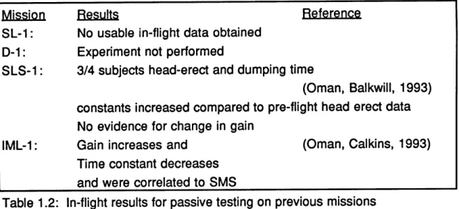
Mission Results Reference SL-1: No usable in-flight data obtained

D-1: Experiment not performed

SLS-1: 3/4 subjects head-erect and dumping time

(Oman, Balkwill, 1993) constants increased compared to pre-flight head erect data No evidence for change in gain

IML-1: Gain increases and (Oman, Calkins, 1993)

Time constant decreases and were correlated to SMS

Table 1.2: In-flight results for passive testing on previous missions

1.3 Previous Engineering Results

On earlier flights (SL-1, SLS-1), the strategy of the SPV data analysis has been to first to take raw eye position and convert it to slow phase velocity. Then two paths have been chosen to further analyze the SPV data. The first path is to fit the SPV data with a model (henceforth called "parametric analysis") and then average and normalize the pre-flight model parameters and the post-flight model parameters, and use a t-test or analysis of variance to test to see if there are statistically significant changes in the model parameters. The second path (henceforth called "ensemble averaging") involved averaging of the SPV time series for two different groups of data. Then statistical tests are performed to determine whether there are significant differences between comparison groups.

In the SL-1 analysis done by Oman and Kulbaski, an acceleration based algorithm was implemented (Massoumnia, 1983), in which the fast phase of nystagmus was detected and then removed from differentiated eye velocity. A first order exponential model was fit to the data by taking the log of the SPV data and performing a linear regression. The data was also ensemble averaged and a chi-square statistical method was used to find statistical differences between selected subsets. A chi-square test is a way to tell if two ensemble averaged time series are significantly different from each other. To do this a chi-squared value is calculated.

(12)

2 (Yi -- xi)2

2 = _(1.6)

i=1 0 _p

where X2 is the chi-square statistic, op2 is the pooled variance, N is the number of degrees of freedom, and xi and yi are the ensemble averaged time series being compared at time i. Then this value is compared to a chi-square

distribution. If the calculated chi-square value is much greater than N then the average squared difference between the two time series is greater than the pooled variance. Since the distribution of chi-square is known, it is possible to test whether the two time series are significantly different. The assumptions that the chi-square test makes are that the number of degrees of freedom is large, and the successive samples are not correlated. (Kulbaski, 1986)

In the D-1 analysis, the eye position was obtained be electronic

differentiation of low pass filtered horizontal EOG data. Then the average SPV was found by manual sampling from the eye velocity chart records at 0.5

second intervals. The differentiator gain was calibrated by reference to the EOG position signal. Gain and time constants were not calculated. For the statistical tests, the SPV time series were ensembled averaged compared using the same chi-square method. (Oman & Weigl, 1990)

In the SLS-1 analysis a new method to determine the slow phase velocity was used. The problem with the Massoumnia acceleration based algorithm was that 10-50% of the fast phase beats were missed, and the data had to be manually edited to remove these artifacts. A completely automated algorithm - order statistic filtering (Engelken, Stevens, 1990) was adopted. First the position data is filtered using a predictive median hybrid filter, which

removes much of the high frequency noise. Second the data is digitally

differentiated. Lastly the data is filtered using an asymmetrically trimmed mean statistical filter, which extracts the SPV envelope by assuming that the eye spends more time in the slow phase than in the fast phase. It was found that this algorithm worked well. It was found, however, that dropouts, which were when the eye instantaneously goes to zero velocity for reasons such as

drowsiness and lack of attention, still remained. An automatic dropout detection algorithm based on a logarithmic linear regression was developed. (Balkwill, 1992)

The remaining data was ensembled averaged, but it was determined that the chi-square test may not have been sufficiently conservative. For a low

(13)

number of runs, which is inherent in space physiology, the sum of the

differences squared will not be distributed like a chi-square distribution. It will be distributed like a sum of t2 distribution. The problem with this is that sum of t2 distribution had not been calculated, so a monte carlo simulation was set up to determine the distribution. (Pouliot, 1991)

A Raphen-Cohen model was fit to the data, and averaged, with statistical significant differences found using a t-test. (Oman & Balkwill, 1993)

After the SLS-1 analysis it was desired to re-analyze the D-1 and SL-1 data sets using OS-filters. The SL-1 data set was selected to be analyzed first. D-1 re-analysis is planned for the future. OS filters were used to calculate slow phase velocity, and the automatic dropout detection algorithm was used.

Ensemble averaging and testing using a sum of t2 test was utilized. Models that were fit to the data included a first order exponential model, velocity

storage/adaptation model, and a fractional exponent adaptation model (Landolt and Correia, 1980). The analysis pipeline from eye position to model fitting was quasi-automated (Liefield, 1993)

The IML-1 analysis was somewhat similar to the SLS-1 analysis. OS filters were used to calculate slow phase velocity, and the same automatic dropout detection algorithm was used. Instead of using more complicated

models like the Raphen-Cohen model, only a first order exponential model was employed, using a log-linear regression method. The rationale behind this was that in the SL-1 re-analysis, it was found that the more free parameters a model

had, the more variable the parameters, and the more difficult to determine statistical significance (Liefield, 1993). So since the VOR response is quasi-exponential it was believed that a simple quasi-exponential should capture the major trends of the data. The gain and time constant from this model were normalized with respect to the subject, run direction, and per or post rotatory phases, based on the pre-flight mean value, in order to combine subjects to increase the

apparent number of runs. Then a two-way ANOVA with replications was used to find statistically significant differences. (Oman, Calkins, 1993)

In all the previous missions to date, the amount of time to process the data was enormous. This was in part due to the limited power of the computers at the time, and part to lack of automation of the analysis pipeline. It would take many months after the mission in order to even have a preliminary idea of what the results would be. In this analysis it was desired to make the analysis

pipeline work near real-time, so that if the astronauts or investigators wanted to,

(14)

they could look at the data after testing to see if responses were back to normal. Also if any decisions needed to be made about how to spend the limited

available post-flight testing time, an informed decision, based on the data, could be made. For example if in the early post-flight period, the NASA administrators tell experimenters that they have only a certain amount of astronaut testing time, time could be better allocated to subjects, and or testing conditions, which would optimize the testing, since the experimenters would have some sense of how the subjects were performing in the experiment.

1.4 Goals of Thesis Research

The goals of this thesis were to analyze and draw conclusions of a very large database of EOG data taken from the SLS-2 mission of the space shuttle, and to continue the evolution of the analysis and statistical algorithms so that the analysis and preliminary statistical testing can be completed in near real time. The important science related question were:

1) How did subject's pre-flight head erect VOR responses compare with results from previous studies ?

2) How did the head-erect SPV response change in parabolic flight ? 3) How did the head-erect SPV response change in prolonged

weightlessness ?

4) How did the head erect SPV response change post-flight ?

5) Was the pre-flight dumping response consistent with previous studies ? 6) How did the dumping SPV response change in prolonged

weightlessness ?

7) How did the dumping SPV response change post-flight ?

8) Did near-real time SPV analysis facilitate decision making during testing ?

9) Are there any recommendations for future analysis and future studies ?"

(15)

Chapter

2: Experimental

Methods

2.1 Subjects

Subjects used in this experiment were five crew members of the STS-58 Space Life Sciences - 2 mission of the Space Shuttle Columbia. There were 3 males and 2 females ranging in age between 36 and 51. The subjects were assigned a random subject code to maintain confidentiality. Their codes were T, V, W, X, and Y. All subjects were free of any vestibular disease. However subject T had esophoria, reduced acuity in the right eye, and a history of

childhood strabismus surgery in that eye. For two of the subjects this was their first time in space.

Preflight testing occurred on four separate days. They were L 122 (BDC1, meaning baseline data collection session #1), L 110 (BDC2), L -88 (BDC3), and L- 18 (BDC4), where for example "L - 122" means 122 days before launch. "Early post-flight testing" occurred on R+0 (BDC5), R+1 (BDC6), R+2 (BDC7), where for example "R+2" means 2 days after landing. "Late post-flight testing" was performed on R+6 (BDC8), R+9 (BDC9), R+1 1 (BDC10). All pre- and post-flight testing took place at Johnson Space Center in Houston Texas. Not every subject was tested on each testing day and table 2.1 shows which days each subject was tested.

One of the subjects who had flown previously had been tested on the earlier mission. For this subject, the preflight database included two sessions (L-122, L-18) from this flight, and four preflight sessions from the previous flight.

In-flight testing occurred on two different days. They were flight-days 4 and 10. The testing occurred in the Spacelab.

Parabolic flight testing occurred on L-129. The testing occurred on a NASA KC-135 aircraft.

Subject W was not available for in-flight and parabolic flight testing, and this subjects' preflight and post-flight VOR responses were highly variable, with a high proportion of dropouts, because the subject often found the testing provocative. Because of this high variability, the likelihood of a statistically significant pre/post-flight comparison was deemed small. Since the focus of this thesis was the comparison between preflight, parabolic flight, in-flight, and post-flight results, Subject W's data was not included in this analysis.

(16)

Sub. L-122 L-110 L-88 L-18 R+O R+1 R+2 R+6 R+9 R+11 T x x x xx x x x V x x x x x x x x x W x x x x x x x x x x X x x xx x x Y x x x x x x x x x x

Table 2.1: Ground Test Matrix (x = single test session, xx = double test session)

Table 2.2: KC-135 and Flight Test Matrix (x = single test session)

2.2 Ground Equipment

Ground testing was conducted using a motorized, computer-controlled rotating chair. The chair could accelerate/decelerate a Aw of 120 deg/sec within 0.5 seconds. The setup was capable of maintaining a chair speed of 120 deg/sec within +/- 2.5 deg/sec.

Eye movements were recorded by an electro-oculography (EOG) system which included neo-natal electrodes, an EOG amplifier (10 x), a low-pass filter (3rd order, 30 Hz cutoff), and a Macintosh Ilci computer, running the Labview software package developed for data acquisition (Liefield, 1993), which sampled the data (120 Hz).

A tape recorder was used to record voice conversations for each testing session. For in-flight, parabolic flight, and early post-flight sessions a video-record of the session was made.

(17)

2.3 Ground Experimental Protocol

The procedure used was similar to that on SLS-1. Subjects were fitted with 5 electrodes at least fifteen minutes prior to testing. This allowed ample time for the electrodes to settle. The horizontal EOG signal was measured by two electrodes, one placed on each outer canthus. The vertical EOG signal was measured by two electrodes, one placed below the right eye and one above the

right eye. Both the horizontal and vertical EOG signals were referenced to an electrode placed on the neck.

The subject was then seated in the rotating chair and given red goggles to wear, whose purpose was to stabilize the corneo-retinal potential. The

subject was also given headphones to wear that would allow the researchers to communicate with him while minimizing ambient sound cues.

Gaze instructions were then given to the subjects. They were told to keep their eyes open and try to stare straight ahead and try not to spot imaginary targets on the walls of the room.

There were four testing options. They were calibrations, spontaneous nystagmus checks, head-erect runs, and dumping runs.

- A calibration consisted of the subject facing a wall. The wall mounted targets subtended +/- 10 degrees both horizontally and vertically. The subject was then told to look at the calibration targets in the following order: Center -Right - Center - Left - Center - Up -Center Down Center Right Left Right -Left -Right - -Left - Right - -Left -Right - Left - Right - Left.

- A spontaneous nystagmus check consisted of having the subject place covers over the goggles and then having the subject stare straight ahead for ten seconds and then close his eyes and stare straight ahead with his eyes open for ten seconds.

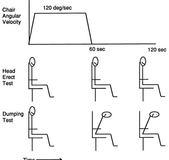
- A head-erect run consisted of the chair spinning at 120 deg/sec for 60 seconds and then the chair would stop and data collection would continue for the next 60 seconds (Figure 2.1). The subject would hold his head so that his neck was straight and the head was in-line with the torso of the body for the entire 120 seconds. The subject was instructed to say "start" when he felt the chair start, "gone" when the direction of spinning sensation was ambiguous, "stop" when he felt the chair stop, and "gone" when the sensation of spinning was ambiguous.

(18)

- A dumping run was like the head-erect run except when the subject feels the chair stop he would say "stop" and the operator would say "down" and the subject would pitch his head 90 degrees forward, and hold it there for the 60 second post-rotatory period. (Figure 2.1)

Chair Angular Velocity Head Erect Test Dumping Test 120 deg/sec 60 sec 120 sec Time

Figure 2.1: Schematic of Head Erect and Dumping Test Procedures

Each time the subject would say "gone" the operator would press a button which would add a pulse to the tachometer signal which would enable the researchers latter to know when the subject said "gone". The delay

between the subject saying "gone" and the operator pressing the button was on the order of 0.5 seconds

Both clock-wise and counter-clockwise runs were performed. The direction of the run was alternated between runs in order to balance residual

(19)

effects of the previous run on the current run since the long time constant of semicircular canal neural adaptation is longer than 60 seconds.

The nominal experimental protocol was as follows: Run 01: Calibration

02: Spontaneous Nystagmus Check 03: CW head-erect run 04: CCW head-erect run 05: CW dumping run 06: CCW dumping run 07: Calibration 08: CW head-erect run 09: CCW head-erect run 10: CW dumping run 11: CCW dumping run 12: Calibration

Run codes were created for computer data files by the following file specification format: SBRR, where S = subject code, B = sequential BDC number, and RR = run number. For example T204, would represent one of subject T's CCW head-erect runs on BDC2 (L-45). KC-135 data had the file specification format: SPBRR, where P indicates that the data was taken in

parabolic flight. In-flight data had the file specification format: SFBRR, where F indicates flight data.

2.4 Differences in Experimental Methods for In-flight and KC-135 Testing

There were several differences between the methods of the in-flight and KC-135 testing vs. the ground testing.

For the in-flight testing the differences were:

a) A manually rotated chair used. The chair was a lightweight Body Restraint System, originally built for 1983 European Vestibular Experiments on

Spacelab-1 (Kass, et al, 1986) which was manually spun to accelerate to the desired speed of 120 deg/sec within 1 second and maintain that speed usually within 10 %. The subjects sat with their legs crossed. A belt mounted digital tape recorder (the Cassette Data Tape Recorder) was used for data collection

(20)

instead of a Macintosh. 2 and 4 K EOG amplifiers were used instead of 10 K. The data was sampled at 100 Hz instead of 120 Hz. There was no middle EOG calibration. There was no tachometer. The angle between the target and the subjects eyes was 9 deg instead of 11.7 deg

For the KC-135 testing the differences were:

a) A lightweight, motorized, servo controlled chair was used. The chair had been developed for similar experiments on Spacelab IML-1 (Oman and Calkins, 1993). The subject's head was restrained by a helmet, which

necessitated monocular (right eye) rather than binocular EOG calibrations, and prevented testing using "dumping" head movements. The angle between EOG calibration targets was 10 deg instead of 11.7 deg. The EOG amplifiers had 2 K gain instead of 10 K gain.

b) Parabolas were flown sequentially, providing alternating periods consisting of approximately 20-25 seconds of 0-G, preceded by a variable interval of 1.0

-1.8 G. For operational reasons, it was not possible to precisely control the duration of the hypergravic interval. During this time, the chair was smoothly accelerated to 120 deg. sec in 2 seconds. Immediately after 0-G was

established, the chair was decelerated in 2 seconds to a stop, and EOG

recording continued for the remaining interval of 0-G. The per-rotatory interval was 46.0 sec (± 5.9 sec SE), and post-rotatory data was recorded for 22

seconds beginning at the onset of 0-G as determined by an accelerometer. Model fitting was based upon 19 seconds of data beginning 3 seconds after the onset of 0-G. The three second delay was incorporated to allow time for the operator to bring the chair to a halt. 1-G control runs were performed with the aircraft on the ground, just prior to flight, using a similar per-rotatory interval (51.4 sec. ± 1.6 sec SE) and an identical 22 sec. post-rotatory recording period. All subjects took scop/dex to reduce their susceptibility to motion sickness and thus maintain alertness.

(21)

Chapter

3: Data Analysis

3.1 Calibration of Eye Position Data

To determine the calibration factors from A/D units to degrees of eye movements, an interactive algorithm was used. (Balkwill, 1992) The horizontal eye position data from the calibrations was shown on the computer screen. Then the expert-user marked 5 regions where the subject was fixating on the right target and then regions where the subject was focusing on the left target. An average value in A/D units was calculated for the right target and then for the left target. The known angle ABC (20 deg),where A = left target, B = subject's head, C = right target was divided by the difference in values between the left and right targets in A/D units This value was the calibration factor for the

calibration run. Usually three calibration runs were performed per session. To get a more accurate calibration factor for each individual run a linear

interpolation was performed between calibration runs. This was an estimate of the calibration factor for the run. (Balkwill, 1992)

3.2 Calculation of Slow Phase Velocity

Two order statistic filters and one linear filter was used to calculate the slow phase velocity from the eye position data. An order statistic filter is a non-linear digital filter which uses a sliding window of odd-length of the input data samples. The input data samples are rank-ordered and the ordered samples are linearly weighted. A linear combination of the ordered statistics constitutes the filter output. The first ordered statistic filter is called a predictive finite-impulse response median hybrid filter (PFMH) which smoothes the input data while preserving saccadic transitions. The linear filter is differentiating filter whose purpose is to calculate eye velocity from eye position. The second order statistic filter is called an adaptive asymmetrically trimmed mean filter (AATM) which extracts the slow-phase velocity from the total eye velocity (Figure 3.1)

(Engelken & Stevens, 1990)

(22)

Slow Phase

Eye Position PFMH Differentiating AATM Velocity

Filter - p Filter N- Filter

Figure 3.1 Block Diagram for calculation of slow phase velocity from eye position

3.2.1 PFMH Filter

The PFMH filter uses an odd length sliding window of length 2N + 1. The first N samples are used to calculate the forward predictor, Xf. The last N

samples are used to calculate the backward predictor, Xb. For a first order FIR predictor the N samples are given weights that linearly depend on its position, with the sample farthest from the N+lst sample given the least weight, and the sample closest to the N+lst sample given the greatest weight. The median of the forward predictor, backward predictor, and the N+1st sample is the output of the filter.

This filter assumes the data is a combination of a root signal and some undesired noise. Repeated use of the PFMH filter will remove the noise,

however for data-sets with a high noise/signal ratio the root signal obtained may not be the desired root signal. (Engelken, 1990)

For this experiment two filters were used of lengths N=6 and N=10, and each filter made two passes on the data. The values for N were the ones used on SLS-1 and were based upon the duration of the fast phases being around

50-100 ms.

3.2.2 Calculation of Eye Velocity.

Eye velocity was calculated from PFMH filtered eye position by using a linear nine point FIR velocity filter consisting of a three point differentiating filter convolved with a seven point low pass filter with a 10 Hz corner frequency (Massoumnia, 1983).

(23)

3.2.3 AATM Filter

The key assumption in the AATM filter is that the eye spends more time in the slow-phase than in the fast-phase. The filter uses this fact to extract the slow-phase velocity from the total eye velocity. A frequency histogram is calculated in the window and the dominant mode is assumed to indicate the SPV. The output of the filter is an average of the velocity samples in the neighborhood of the dominant mode. (Engelken, 1990)

3.3 Tachometer Analysis

The tachometer signal needed to be analyzed in order to extract some necessary information with respect to rotation of the chair. This information was the delay, spin length, run length, and spin velocity. An algorithm was

developed to find these important parameters. (Pouliot, 1992) The algorithm basically looked for large changes in the tachometer signal which will occur at the chair start and stop. The first large change will be assigned the chair start and the second will be assigned the chair stop. From this information, the rest of the parameters can be calculated.

For the in-flight data collection, there was no tachometer signal, so the start and stop points were determined manually by looking at the record of the chair yaw accelerometers, and looking at the EOG data and looking for the first saccades.

3.4 Outlier Detection and Removal

The length of each per-rotatory and post-rotatory section had to be normalized to 60 seconds. If the run segment was less than 60 seconds then the median of the previous 5 samples was added to make the run segment 60 seconds. If the run segment was greater than 60 seconds then data beyond 60 seconds was truncated. In order to remove dropouts, an automated algorithm was developed. (Balkwill, 1992) The basic idea in this method is to look at the natural logarithm of the data and then perform a least squares linear fit. The root-mean square error (RMS) about the line was calculated, and any data point greater than 3*RMS or below 7.4 deg/sec, along with all points within 1/2

second, were marked as bad. A new linear fit was performed based upon the

(24)

data with the previous bad sections ignored. However the RMS is calculated based upon the whole data-set, and then the process is repeated. When the RMS of the current fit converges to within 20% of the previous RMS value then the bad sections are designated as dropouts.

3.5 Decimation

It was desired to decimate the data from a sampling rate of 120 Hz down to 4 Hz in order to save computation time and disk space. In order to do this the 120 seconds of 120 Hz data was broken down into 30 equal segments and then the mean and variance of each segment was calculated. This information was saved as the decimated data. (Balkwill, 1992) In a similar manor, the in-flight 100 Hz data was decimated down to 4 Hz.

3.6 Model Fitting

It was desired to fit a first order exponential to the decimated data. To do this constrained optimization was used in order to obtain the fit that minimized the RMS between the data and the model fit. (Liefield, 1993) The per and post rotatory data were fit separately since the per and post rotatory segments

should be asymmetric due to the long adaptation time constant being around 80 seconds. The model thus yielded a gain and time constant for both the per and post rotatory phases

(25)

3.7 Run Segment Rejection Criteria

In some cases, dropouts can be prolonged, and the model fit is based on a relatively small sample of SPV data. It is probably inappropriate to average the model fits based on small amounts of data, runs containing large electrode motion related SPV artifacts, or responses where SPV response was virtually absent due to fatigue with other data where this was not the case. A

quantitative run-rejection criterion was developed, and applied uniformly across all subjects and all conditions. For some of the previous missions a quantitative run rejection rule was not used. For example in SLS-1 the run rejection

criterion was "the SPV envelopes were examined visually, and discarded if appropriate." (Balkwill, 1992) This could conceivably have lead to an added

bias due to experimenter prejudice.

In determining the criterion, histograms of the parametric data were examined. It was determined that atypical run segments with extreme outliers or a virtually absent per- or post-rotatory response could usually be identified by

using the following criteria:

1) The model-fitting routine hit a lower bound. (K < .06) or (T < .15) 2) Percent good of a run segment was less than 60%.

3) Mean-square error was greater than 200.

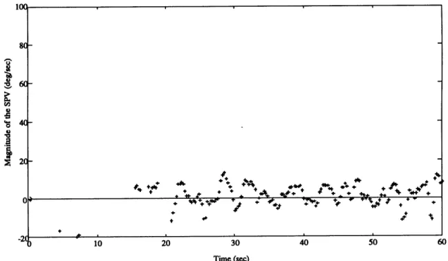
The rationale behind the first criterion was that if the model fitting routine hit a lower bound then the run parameters were not physiological realistic for a 120 deg/sec step response. This might occur for example if the subject showed little response for most of the run. (figure 3.2)

The rationale behind the second criterion was that if over 40% of the first 25 seconds of the run segment had been discarded by the outlier detection algorithm than not enough data is there to make any further conclusions based upon this run segment. (figure 3.3)

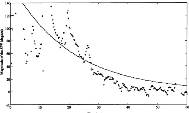
The rationale behind the third criterion was that if the mean-square error was greater than 200 than the data was extremely noisy and should not be used. (figure 3.4)

(26)

1n(~

a _4C

-10 20 30 40 50

Time (sec)

Figure 3.2: Example of model-fitting routine hitting a lower bound (Model fit is the black line). Low frequency SPV oscillations are typical of a sleepy subject.

100 80 40-20- + 0,- 4., N 4.+ .+ -20 60 70 80 90 100 110 12 Time (sec)

Figure 3.3: Example of % good < 60 % (Actual % good = 35 %)(Model fit is th black line)

0

Page 26

(27)

* +

80-

-Soo

Figure 3.4: Example of MSE > 200 (Actual MSE = 1370)(Model fit is the black

line) _4. ₊ ₊ ₊

4.-

0-(510 20 30 40 50 60

Time (was below 25 deg/sec.c)

Figure 3.4: Example of MSE > 200 (Actual MSE

=

1370)(Model fit is the black

line)

It was decided that if one of the run-rejection criteria was met, than both

the gain and the time-constant of the run-segment should be thrown out due to

the direct relationship between the gain and time-constant.

These criterion differed a little from the previous missions in which a

quantitative run rejection criterion was used. In IML-1 (Oman & Calkins, 1993),

the run rejection criterion was to remove all outliers in the histogram distribution

greater than 2 SD's. But in looking at the individual runs it was found that some

runs that were in the middle of the distribution were unreliable since for

example, if there were a lot of dropouts, the model fitting routine could give

unreliable results. In the SL-1 re-analysis (Liefield, 1993), the criterion was the

following:

1) more than 10 seconds worth of data was removed from a run

segment.

2) The model fitting routine hit a constraint (.18

<

K < 1.8) or

(5 < T < 45)

3) Peak SPV response was below 25 deg/sec.

(28)

The first criteria is the same the SLS-2 criterion #2, since 40% of 25 seconds (the number of seconds the % good statistic was based on) is 10 seconds. The second criteria is similar to the SLS-2 criteria #1, however it was decided to reduce the lower bound in order to not throw away low gain data, and .06 is very much below what is considered to be physiologically reasonable. The third criterion was not used, for the same reason why the lower bound was reduced, for it was not desired dismiss low gain responses, and in Liefield's thesis, as an afterthought he questioned the justification of this rule.

3.8 Near real-time statistical analysis

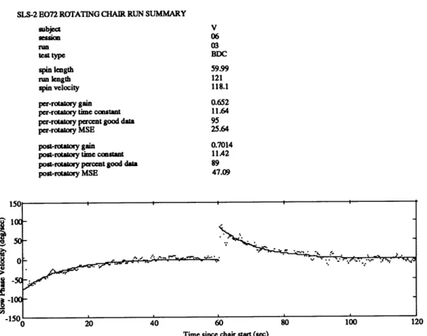
It was desired to calculate some statistical parameters in near real time during the post-flight BDC sessions in order to obtain a basic understanding of how the subjects were performing in the experiment. Two different ways of looking at the data in near real-time were developed. The first was to look at individual run reports (Figure 3.5), as was done by Oman and Calkins (1993), except that the results were fit by a model (Eqn 1.5), superimposed on the data, and the mean square error was also calculated. The second way was to

calculate histograms (Figure 3.6), means, and variances, of the parametric data.

(29)

SLS-2 EO72 ROTATING CHAIR RUN SUMMARY subject V session 06 run 03 test type BDC spin length 59.99 run length 121 spin velocity 118.1 per-rotatory gain 0.652 per-rotatory time constant 11.64 per-rotatory percent good data 95

per-rotatory MSE 25.64

post-rotatory gain 0.7014 post-rotatory time constant 11.4A2 post-rotatory percent good data 89 post-rotatory MSE 47.09

150

-100-0-1500

020 4060 10 120

Time since chair start (sec)

Figure 3.5: Example of a run report for one of subject V's early post-flight runs.

14 12 10 c 8 6 --₄

2

0 o Il 0 2 4 6 8 10 12 14 16 18 20 22 24 26 28 30

Bin (Time constant (sec))

Figure 3.6: Example of a histogram for Subject V's early post-flight per-rotatory time constants.

The calculation of the histograms, means, and variances was performed

by exporting the parametric information describing each run from Matlab to

(30)

subject session run # test type direction type of run delay run length spin length spin velocity calibration # V 6 3 BDCO C FE 1.04 121 59.99 118.1 0.1199 V 6 4 BDC OCW FE 1.03 121 60.01 -119.1 0.1188 V 6 5800 MON DMP 1.03 121 60.01 118.1 0.1178 V 6 6 800C OW DMP 1.03 121 60.01 -119.0 0.1168 V 6 8 BOC CN FE 1.05 121 59.98 118.1 0.1142 V 6 9 BDC OCW -E 1.04 121 59.99 -119.1 0.1127 V 6 10 BDC ON DMP 1.04 121 59.99 118.1 0.1111 V 6 11 BDC OCW DAP 1.04 121 60.03 -118.9 0.1095 V 7 3 BDC ON lE 1.03 121 60.01 118.1 0.1121 V 7 4 BDC OcW FE 1.04 121 60.01 -118.9 0.1115 V 7 5 BDC CN DAP 1.04 121 60.00 118.2 0.1109 V 7 6 BDC CON DMP 1.03 121 60.00 -118.9 0.1103 V 7 8 BDC CWN E 1.04 121 60.00 118.2 0.1052 V 7 9 BDC OCW HE 1.04 121 60.01 -118.9 0.1007 V 7 1 0 BDC CON DP 1.03 121 60.00 118.2 0.0963 V 7 11 BDC ONW DMP 1.03 121 60.01 -118.9 0.0918

subject session run # per- % good per-rot gain per-rot t.c. per-rot MSE post - % good post-rot gain post-rot time constant post-rot MSE

V 6 3 95 0.65 11.64 25.64 89 0.70 11.42 47.09 V 6 4 83 1.20 6.67 36.99 76 0.48 14.13 52.61 V 6 5 86 0.92 9.15 37.76 63 1.05 5.79 16.34 V 6 6 83 0.87 7.77 27.40 59 0.06 0.15 102.80 V 6 8 91 0.60 11.34 49.16 76 0.85 11.84 49.98 V 6 9 62 0.75 8.29 66.43 76 0.94 10.74 52.24 V 6 10 88 1.01 9.50 33.34 77 0.86 6.04 31.22 V 6 11 100 0.74 10.41 57.30 53 0.71 5.81 19.48 V 7 3 72 0.69 9.14 25.29 83 0.48 14.08 25.76 V 7 4 36 0.06 0.15 55.77 85 0.72 11.33 33.18 V 7 5 85 0.79 9.87 22.23 65 1.05 4.50 23.91 V 7 6 71 0.43 10.19 46.84 78 0.61 8.88 25.96 V 7 8 84 0.99 8.34 19.24 66 0.92 8.23 42.26 V 7 9 52 0.61 6.85 37.01 49 0.90 10.71 26.08 V 7 10 82 0.52 11.61 30.79 70 0.91 5.98 16.59 V 7 11 67 0.95 8.24 24.69 72 0.77 7.19 14.19 a) a) -u CL a) U) 0 E u 0) cm iz

(31)

Microsoft Excel. This information included for both the per and post-rotatory segments: subject (T, V, X, or Y), BDC # (1-10), chair direction (cw or ccw),

post-rotatory head condition (he or dmp), percent good, gain, time constant, and mean square error. (Figure 3.7)

Then templates were made for each subject in Excel so that histograms, means, and variances could be calculated. A template is a Excel worksheet with all the columns and rows labeled, the formulas already calculated, and the graphs set so when the data is imported all the statistical calculations and

histograms could be performed. The templates for each subject was made for pre-flight, early post-flight, and late post flight in order to calculate histograms, means, and variances for different subsets of the data. Preflight included BDC's 1-4, early post-flight BDC's 5-7, and late post-flight BDC's 8-10. The subsets were per-rotatory gain, per-rotatory time-constant, head-erect post-rotatory gain, head-erect post-rotatory time-constant, dumping post-rotatory gain, dumping post-rotatory time constant.

Using the macro programming language in Excel was studied but it was determined to be not feasible to use since it did not allow any flexibility of a real programming language but rather it was a string of pre-determined commands. In the future when a more suitable macro programming language becomes available it would be better to use this rather than the templates.

3.9 Statistical Comparisons of the Data 3.9.1 Kolmogorov-Smirnov Test

The Kolmogorov-Smirnov (KS) non-parametric test determines if two cumulative frequency distributions (A, B) came from the same population. It asks how probable it is that the greatest observed difference in their respective cumulative frequency distributions (CFD):

ks = maxlCFD(B) - CFD(A)I

(3.1)

would occur if the distributions A and B, were really the same. (Siegel, 1956) The KS test was used to test pairs of sequences of parametric data, and pairs of SPV time series. The KS test can (in part) determine if one curve decays faster than another if both start from the same value, and assuming both decay

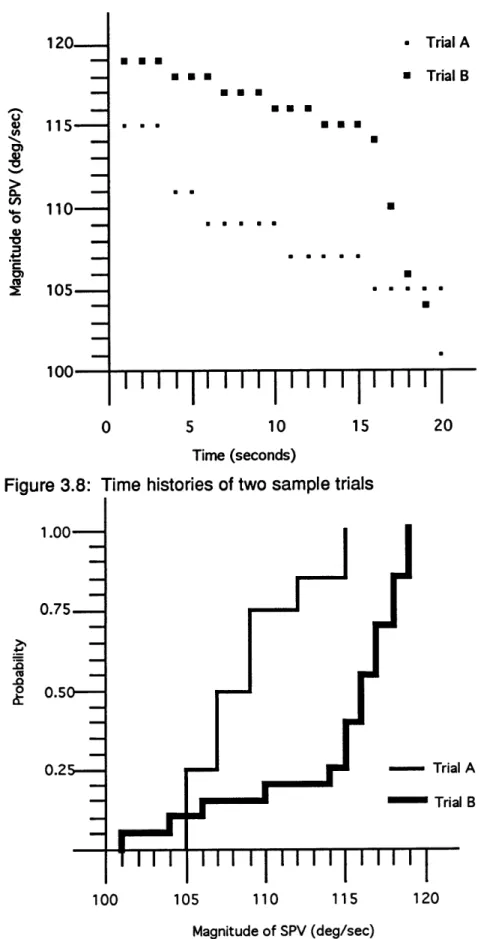
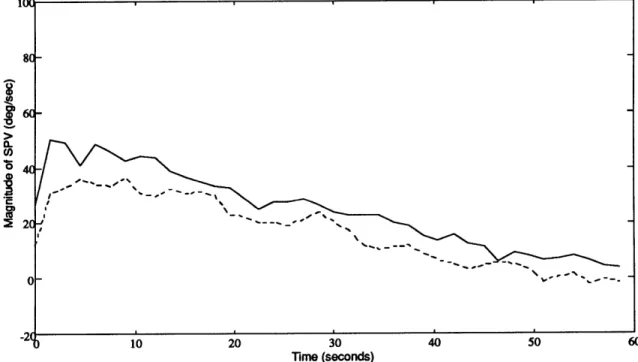
exponentially. The example below (Natapoff, 1994, personal communication)

(32)

shows the time histories of two hypothetical SPV curves (Figure 3.8) and their corresponding cumulative frequency distributions (Figure 3.9). The maximum difference (13 x 0.05 = 0.65) in the CFDs occurs at x = 112. A total of (4, 17)

measurements of (A, B) lie below x = 112. Thus the difference at x = 112 is 13 out of the 20 points in each set. Since the two-tailed KS test has a critical value of 11 at the a = 0.01 confidence level, the CFDs are significantly different.

This use of the KS test can not detect certain types of differences. It will not, for example, distinguish one permutation of a set of numbers from another, and therefore is not sensitive to the time sequence of these numbers. For example, the same sequence occurring in inverted time order would be

indistinguishable from the original, and long sequences that converge to the same value. In this experiment, the KS test was used to compare ensemble average SPV responses under different conditions. 60 second long sequences were used, except that a shorter interval was used for both when the

comparison involved flight data.

(33)

120-- 115- 110- 105-100 U.. U E * Trial A * Trial B N N N E 0 0 U a U a a U• 1I~ 20 Time (seconds)

Figure 3.8: Time histories of two sample trials

1.00'

0.75.

0.2!

100 105 110 115 120

Magnitude of SPV (deg/sec)

Figure 3.9: Cumulative Frequency Distribution

Page 33

I

I I I

I

I I I I I

i * a a a a * S * *

(34)

3.9.2 Two-Sample t-Test for Independent Samples

The parametric data was compared by referring the t-statistic to the two tailed student t-distribution for nl + n2 - 2 degrees of freedom.

X

1

-X

2 t

=

X 2 (3.2)

1 (s

-

+

-where

S

(nl - 1)s + (n

2

- 1)s

2

(3.3)

S

=

(3.3)

n, +n

2

-2

3.9.3 Sum of T-square statistic

The statistic below would be distributed as x2 if xi, yi are based on averages of large number of measurements and if the measurements for different values of i were independent. These assumptions were made in the analysis of earlier missions, D-1 and SL-1. However for the AATM algorithm, which uses a 1 second moving averager, adjacent samples at 4 Hz are correlated. A new sampling frequency at which adjacent samples to be

independent was found by looking at the auto-correlation of one subject's data. The auto-correlation with a delay of 1.5 seconds was found to be small if a new sampling rate of 2/3 Hz was used. Then the sum of t2 statistic was calculated:

,

t

2 _. _(Yi _xi) 2

(3.4)

i=l Gp

Since the distribution of this statistic (as opposed to x2 ) is not readily available, it was used qualitatively. A very large sum of t2 would suggest a significant result, while a low sum of t2 would suggest a non-significant result.

By looking at a large number of t2 values and comparing them to the plots of the actual data, and other statistical tests, it was determined that a sum of t2 of 1000 would be the breakpoint between the two above mentioned trends.

(35)

3.9.4: Actual use of the statistical tests

Responses under two different conditions were compared using six statistical tests. The t-test and KS test were both performed on the gain and time constant parametric data. Both the sum of t2 and KS tests were performed

on the ensemble averaged data. A rule of thumb was adopted to determine if the results of the two comparisons taken together indicated a real difference. If

either the gains or time constants were found to be significantly different by the t-test, and if the KS test for the ensemble average data also indicated a

significant difference, then the two cases was determined to be different. The other two tests, i.e. KS test for the parametric data, and the sum of t2 data for the ensemble data were used as secondary indicators.

(36)

Chapter

4:

Results

4.1 Completion status of runs

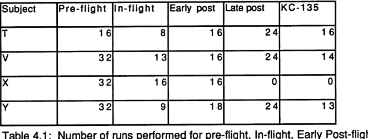
The number of runs performed per subject varied. Reasons why some runs were not performed included time constraints, nausea of the subject, operator error, and equipment malfunctions. Table 4.1 lists the number of runs performed for each subject during the pre-flight, in-flight, early post-flight, late post-flight, and KC-135 testing periods.

Subject Pre-flight In-flight Early post Late post KC-135

T 16 8 16 24 16

V 32 13 16 24 14

X 32 16 16 0 0

Y 32 9 18 24 13

Table 4.1: Number of runs performed for pre-flight, In-flight, Early Post-flight, and the KC-135

4.2 Run rejection results

As outlined in section 3.7, three run segment rejection criteria were used. The results of these criteria are listed in tables 4.2, 4.3, 4.4, and 4.5 for the pre-flight, in-pre-flight, early post-pre-flight, and KC-135 testing periods. The first column is the percent rejected category which is the total number of run segments

rejected divided by the total possible number of run segments. A run segment differs from a run since a run is composed of both a per-rotatory and

post-rotatory segment, while a run segment segment is either a per-post-rotatory segment or a post-rotatory segment. The next three columns are the categories

constraint hit, % good < 60, and MSE > 200, which are the three run rejection criteria outlined in section 3.7. The percentage listed for these three categories is the percentage of the rejected run segments that this run segment rejection criteria was used. There is some overlap in these categories, e.g. one run segment might hit a constraint, and have a % good < 60. However the run

(37)

rejection routine first used the constraint hit criteria, then the % good on the remaining segments, and finally the MSE criteria. Hence the relatively low percent rejected using the MSE criteria was in part due to the order in which the criteria were applied.

Subject Percent Rejected Constraint Hit % good < 60 MSE > 200

T 66 % 52 % 48 % 0 %

V 19 % 17 % 83 % 0 %

X 77 % 65 % 35 % 0 %

Y 27 % 18 % 70 % 12 %

Table 4.2: Results of outlier detection for pre-flight

Subject Percent Rejected Constraint Hit % good < 60 MSE > 200

T 19 % 100 % 0 % 0 %

V 15 % 100 % 0 % 0 %

X 13 % 100 % 0 % 0 %

Y 0% 0% 0% 0%

Table 4.3: Results of outlier detection for in-flight

Subject Percent Rejected Constraint Hit % good < 60 MSE > 200

T 47 % 67 % 33 % 0 %

V 13 % 50 % 50 % 0 %

X 84 % 85 % 15 % 0 %

Y 33 % 25 % 67 % 8 %

Table 4.4: Results of outlier detection for early post-flight

(38)

Subject Percent Rejected Constraint Hit % good < 60 MSE > 200

T 25 % 75 % 25 % 0 %

V 7% 100 % 0% 0%

Y 15 % 50 % 50 % 0 %

Table 4.5: Results of outlier detection for KC-135

One interesting conclusion that can be drawn from the run rejection results is that for all subjects and especially subject X, the percent rejected during in-flight and in the KC-135 was less than the pre-flight.

4.3 Near Real-Time Analysis Experience

The purpose of the near real-time analysis was so the experimenters could have an idea of how the data looked. Complete analysis of one session on four subjects typically required 4-7 hours of computing on a Macintosh Quadra. User interaction was required for EOG calibration analysis. However

most of the subsequent processing which was automated in batch mode, using the method developed in Matlab by Liefeld (1993). Run reports were

automatically generated. Data was then manually exported to Excel

spreadsheets for rapid histogram generation and statistical analysis. On prior missions, this analysis took several days of interactive work. During preflight testing, analysis was performed at MIT between test sessions. During post-flight testing, data was analyzed at Johnson Space Center, and results from a given day's session were generally available the next day. The histograms, means, and variances were useful to see if the subjects data appeared normally distributed, and to see if there were any trends in the data as compared to pre-flight norms. The run reports which showed both the SPV envelope and the

model parameters proved useful in keeping the experimenters in touch with the actual data from each run, to see if any runs were abnormal, and in planning for subsequent preflight test sessions. The use of the near real-time analysis was apparent preflight, in-flight and early post-flight.

In preflight testing, one subject asked if they could be excused from two test sessions, since test data for this subject was available from a previous

Changes in the horizontal angular vestibulo-ocular reflex of SLS-2 space shuttle astronauts due to weightlessness