HAL Id: hal-00502329
https://hal.archives-ouvertes.fr/hal-00502329
Submitted on 15 Jul 2010
HAL is a multi-disciplinary open access
archive for the deposit and dissemination of
sci-entific research documents, whether they are
pub-lished or not. The documents may come from
teaching and research institutions in France or
abroad, or from public or private research centers.
L’archive ouverte pluridisciplinaire HAL, est
destinée au dépôt et à la diffusion de documents
scientifiques de niveau recherche, publiés ou non,
émanant des établissements d’enseignement et de
recherche français ou étrangers, des laboratoires
publics ou privés.
Dynamics of a ball bouncing on a vibrated elastic
membrane
Brice Eichwald, Mederic Argentina, Xavier Noblin, Franck Celestini
To cite this version:
Brice Eichwald, Mederic Argentina, Xavier Noblin, Franck Celestini. Dynamics of a ball bouncing
on a vibrated elastic membrane. Physical Review E : Statistical, Nonlinear, and Soft Matter Physics,
American Physical Society, 2010, 82 (1), pp.016203. �hal-00502329�
B. Eichwald, M. Argentina†, X.Noblin and F. Celestini∗
Universit´e de Nice Sophia-Antipolis, Laboratoire de Physique de la Mati`ere Condens´ee,
CNRS UMR 6622, †Universit´e de Nice Sophia-Antipolis,
LJAD CNRS UMR 6621, Parc Valrose 06108 Nice Cedex 2, France (Dated: July 15, 2010)
We investigate the dynamics of a ball bouncing on a vibrated elastic membrane. Beyond the classical solid/solid case, we study the effect of introducing new degrees of freedom by allowing sub-strate oscillations. The forcing frequency of the vibration strongly influences the different thresholds between the dynamical states. The simple model proposed gives a good agreement between the experiments and the analytical expression for the threshold at which the ball begins to bounce. Numerical simulations permit to qualitatively recover the experimental phase diagram. Finally, we discuss how this simple system can give new insights in the recent experimental studies on bouncing droplets.
PACS numbers: 05.45.pq, 45.55.Dz
I. INTRODUCTION
In this communication we study a variation of the clas-sical bouncing ball (BB) experiment [1–3]: a rigid and massive ball is forced to bounce against a vertical and periodic oscillation of an infinitely heavy and rigid sub-strate. Despite the simplicity of this experimental set-up, a complex phenomena arises: chaos is manifested, as theoretically predicted previously in [4], through a period doubling scenario [5, 6]. Beyond the rigid-rigid case, re-cent experiments have added complexity to the BB prob-lem by using substrates or bouncing objects which are deformable. Using viscous liquids with surface tension effects or elastic solids, these modes of deformation can couple to the bouncing motion. A highly viscous droplet can be kept non-coalescing when impacting against a highly viscous liquid whose recipient is settled into move-ment via vertical and periodic oscillations. As the period of the oscillation becomes of the order of the time nec-essary to drain the air film separating the drop from the substrate, the coalescence is impeded, and the droplet can bounce periodically for a strong enough imposed ac-celeration [7]. The impact of the drop over the viscous substrate may eventually generate waves that induce a drop motion; then a coupling with the substrate defor-mations has to be taken into account when studying such phenomena. When the droplet has a lower viscosity than the viscous substrate, droplet deformations have also to be taken into account to describe the bouncing dynam-ics [8]. Instead of a liquid-gas interface, the substrate can be a thin liquid soap film above which a droplet can bounce, and be driven periodically [9]. We aim here to describe the ”solid” case of this experiment, that is a rigid sphere interacting with an elastic membrane and to look at the effect of the frequency together with the am-plitude. Our purpose is to propose a general framework
∗Electronic address: [email protected]
to study bouncing ball dynamics coupled with an oscilla-tion mode, which originates either from the deformaoscilla-tion of a droplet or the substrate.
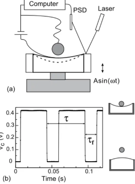
Asin(ωt) 0 0.05 0.1 Time (s) 0 0.1 0.2 0.3 0.4 Vc (V)
τ
τ
f PSD Laser Computer (a) (b)FIG. 1: Experimental set-up (a) and characteristic electric signal (b) detecting the contact between the ball and the elastic membrane
We investigate the dynamics of a rigid ball free to bounce on an elastic substrate accelerated vertically and periodically with a frequency f . This model experiment is able to capture the physical mechanisms that governs the dynamics of the bouncing systems discussed above. Denoting f0 the resonant frequency of the membrane,
the limit case for which f /f0 tends to zero corresponds
to the BB system. We focus here on the effects of this new parameter on the bouncing ball dynamics. We first detail the experimental set-up, then the phase diagram with the different dynamical states observed as a func-tion of the applied accelerafunc-tion and forcing frequency. In a second part, we present a model for which numerical and analytical predictions are compared to the
experi-2 mental results. Despite its simplicity, our model gives a
good agreement between the experiments and the ana-lytical expression for the threshold of detachment of the ball. Numerical simulations allow to explore the phase diagram that appears to be in good agreement with the experimental one. In conclusion, we emphasize the role of the new degree of freedom brought by the substrate de-formations and we address the link between our approach and the different bouncing drops experiments previously presented.
II. EXPERIMENTS
The experimental set-up is presented in Fig. 1a. A thin disk-shaped elastomeric membrane (PolyDiMethyl-Siloxane, PDMS) is clamped on top of an aluminium box. This cylindrical-shape support is hermetically closed by the membrane lying on top of it. This membrane has a diameter of 60 mm and a thickness of 300 µm and can be stretched by varying the air volume below it, which also modifies its mean curvature. The support is fixed to the moving part of a vibration exciter.
A function generator creates a sinusoidal oscillation of frequency f = ω/2π and amplitude A. This signal is am-plified by an audio power amplifier and sent to the vibra-tion exciter. A laser beam reflecvibra-tion over an optical posi-tion sensitive detector (PSD) allows the measurement of the vertical position of the support as function of time. We deduce from this method the acceleration as function of time with a good accuracy for such large displace-ments and low frequencies. The normalized amplitude of the imposed acceleration is Γ = Aω2/g. The steel-made
bouncing bead has a diameter of 1 cm. To characterize the system membrane + ball, we measure the first reso-nance frequency of the free membrane, ω0f = 90 Hz, and
the corresponding frequency of the membrane with the additional mass of the ball, ωc
0= 20 Hz. These resonance
frequencies are measured by searching the maximal am-plitude of oscillations of a laser beam reflecting on the membrane itself. Due to the energy dissipation within the PDMS, the membrane vibrations are damped. The relaxation time of the charged membrane has been mea-sured and is equal to 99 ms.
For sufficiently high vibrational amplitude, the ball bounces on the membrane. The main experimental dif-ficulty is to precisely detect the times when the ball touches the PDMS. In order to provide such measure-ments, a thin Nickel sheet, 3 x 3 mm, is deposited on the center of the membrane. Two thin and light metallic wires are connected to the bead and to the nickel sheet by soldering. Their lightness and flexibility have been cho-sen in order to optimize the electric contact and to reduce the mechanical perturbations. The circuit is closed by a DC generator and the signal is sent to the terminals of an I/O card. As illustrated in Fig. 1b, each time the bead is in contact with the membrane, the measured tension is ≃+0.4 V, while it is zero when the bead is no longer in
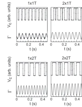
contact. We can therefore accurately measure the time between two successive rebounds, τ , and the time of flight τf. 0 0.2 0.4 t (s) 0.2 0.4 0 0.2 0.4 0 0.2 0.4 1x1T 2x1T 1x2T 2x2T 0 t (s)
Γ
Vc ( arb . uni ts) t (s) t (s)Γ
Vc ( arb . uni ts)FIG. 2: Examples of nxmT bouncing dynamical states. The
period of the ball motion is Tb= n m T , n is the number of
dissimilar times of flight.
We look at the different dynamical states of the ball as a function of ω and Γ. For a fixed frequency, the accel-eration is increased from 0 to the threshold at which the ball bounces in a chaotic way. We study the system for frequencies in between 15 and 30 Hz, around the resonant frequency of the charged membrane (ωc
0 = 20 Hz).
De-pending on ω and Γ the ball can be stuck or can bounce in qualitatively different ways. Examples of bouncing are given in Fig. 2. We use the denomination nxmT to char-acterize the dynamical bouncing state where T = 2πω is the excitation period of the shaker. Below the chaotic threshold, the ball motion is periodic with a period Tb = n m T , n being the number of dissimilar times of
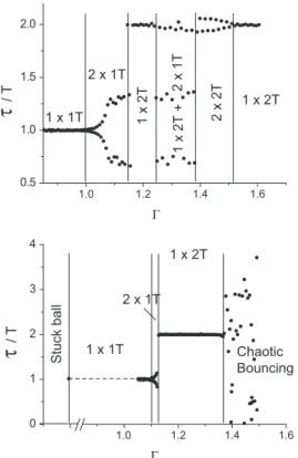
flight and m is such that the product n m corresponds to the periodicity Tb. We present in Fig. 3 two bifurcation
diagrams for two frequencies of 21.5 Hz and 26 Hz. In these diagrams we plot the delay τ between two consec-utive take off as function of Γ and the various dynamical states observed are mentioned. At low amplitude the ball is stuck while the motion is chaotic at large amplitude.
From the bifurcation diagrams, we can determine the different states observed for increasing Γ. We have de-termined such diagrams for varying frequencies, all the states can then be represented as function of frequency and acceleration. The corresponding experimental phase diagram (Γ,ω/ω0) is presented in Fig. 4 The states nx1T
with n > 0 are observed for the classical BB system for sufficiently high amplitude of vibrations. The main effect of the membrane elasticity is to enhance the stability
re-1.0 1. 2 1.4 1. 6 0 1 2 3 4 Γ St u ck b a ll 2 x 1T 1 x 1T 1 x 2T Chaotic Bouncing 1. 0 1.2 1. 4 1.6 0. 5 1. 0 1. 5 2. 0
τ
/ T Γ 2 x 1T 1 x 1T 1 x 2 T 2 x 2 T 1 x 2T 2 x 1 T 1 x 2 T +τ
/ TFIG. 3: Bifurcation diagrams for f = 21.5 Hz (top) and
f = 26 Hz (bottom). We plot the time τ (normalized by
T) between two take off from the membrane as function of Γ.
gion of dynamical states with m > 1. Even if such states have been observed for the BB system, their appearance strongly depends on initial conditions.
III. MODEL AND SIMULATIONS
We now propose a model to describe the dynamics of the ball bouncing on the membrane. In order to capture the physics of the problem with the lowest complexity, we model the membrane response with a spring of stiffness k and a zero length at equilibrium. The mass of the membrane and of the ball are respectively noted mmand
mb. The ball, the membrane and the vibrating support
are respectively located at the heights z2, z1 and z0. A
scheme of the model is represented in the inset of Fig. 5. The balance of the vertical momentum is written with the following relations:
mbz¨2 = −mbg+ r (1)
mmz¨1 = −mmg − r − k(z1− z0) − νi( ˙z1− ˙z0) − νez˙1(2)
z0 = A cos ωt, (3)
where g is the gravitational acceleration, r is the reaction force (r is equal to zero when the ball is not in contact with the membrane) and νi,e are the friction coefficients
associated to the internal and external energy dissipation on the membrane. We write the system in dimensionless variables using the following changes of scale: zi = A˜zi,
0.75 1.00 1.25 1.50 0. 0 0. 5 1. 0 1. 5 2. 0
Γ
1 x 1T 1 x 2T 2 x 2T 2 x 1T + 1 x 2T 4 x 1T 2 x 1T Stuck ball Chaotic bouncing Ω = ω ω0FIG. 4: Experimental phase diagram. The dashed line cor-responds to the analytical model for the threshold between a stuck and a bouncing ball. Full lines are guides to the eye. The two gray vertical lines correspond to the bifurcation dia-gram frequencies in Fig. 3
t = ˜t/ω, r = mbAω2˜r. By dropping the tilde, we get:
¨ z2= − 1 Γ+ r (4) ¨ z1= − 1 Γ− µr − (µ + 1) Ω2 ((z1− z0) + βiΩ( ˙z1−˙z0) + βeΩ ˙z1) (5) z0= cos t. (6)
The dimensionless parameters are : the ratio of masses µ = mb
mm, the normalized acceleration Γ =
Aω2
g , the
parameter βi,e = (mmν+mi,eb)ω0 measuring the dissipation
respectively within and outside the PDMS. The dimen-sionless frequency is Ω = ω
ω0, the later parameter
be-ing the ratio of the forcbe-ing frequency over the reso-nance frequency of membrane charged with the ball : ω0 =
q
k
mm+mb. We now compute the minimal
acceler-ation Γ that allows the detachment of the ball from the membrane. The ball is stuck when z1(t) = z2(t) and by
inserting (4) into (5), we compute the reaction r and we conclude that z2 obeys to a forced oscillator equation:
¨ z2= − 1 Γ− 1 Ω2((z2−z0) + βiΩ( ˙z2−˙z0) + βeΩ ˙z2) (7) r = 1 Γ + ¨z2 (8)
The periodic evolution of z2 is obtained from (6,7):
z2= − Ω2 Γ + s (Ωβi)2+ 1 (1 − Ω2)2+ (Ω(β i+ βe))2 cos(t+ φ), (9) which, for small dissipation terms, presents a maximum amplitude at Ω = 1. The phase φ depends on Ω , βi,e.
4 becomes zero, i.e., ¨z2 = −Γ1c. This defines the critical
acceleration Γc: Γc= s (1 − Ω2)2+ (Ω(β i+ βe))2 (Ωβi)2+ 1 , (10)
this threshold is shown in Fig. 4 and Fig. 5 separating the region where the ball remains on the membrane to the one where the ball reach a 1x1T bouncing state.
z0 z1 z2 g (A, ω) Ω = ω ω0
FIG. 5: Threshold between the stuck and the bouncing ball. Inset : scheme of the model proposed for a bouncing ball on a vibrated membrane.
We represent in Fig. 5 the experimental data for Γcas
a function of Ω together with the analytical expression given in Eq. (8). We use the value ω0 = 20Hz and
βi = 0.08 as measured experimentally (βi = 1/(ω0τ )).
For our system, the external dissipation can be neglected because the drag force from the air on the membrane is very small. It can be evaluated by calculating the energy loss during one period, that is a quality factor Q = 1/(2βe) ≃ (µρpe)/(ρaam) with ρpand ρathe density
of PDMS and air respectively, e the membrane thickness and am the maximal amplitude. Then we have roughly
βe < 5 10−3βi and we use βe = 0. Without any free
parameters, we find a satisfactory agreement between the experimental data and the model. We can clearly confirm that the critical acceleration needed for the ball to bounce is minimal around the resonance frequency of the charged membrane.
The set of equations (4,5,6) can be written as a non linear mapping that gives the positions zi
2and z i+1 2 of the
ball between two successive bouncing events i and i + 1. When the ball is detached from the membrane, r = 0, and the two equations of motion (4,5) can be solved exactly: the ball (resp. the membrane) undergoes a parabolic tra-jectory (resp. a damped oscillatory motion around the position z0). As the ball touches the membrane, r, z1
and z2are found using (7,8). The time ti+1 at which the
ball takes off, is finally obtained for r = 0. Nevertheless, this implicit mapping presents two drawbacks. First, the i + 1 bouncing event has to be computed by solving a
non-linear equation that present several solutions. A spe-cial numerical treatment has to be implemented to select the physical solution. Second, near the threshold detach-ment, there is a critical slowing down of this algorithm due to numerous small jumps of the ball. Therefore, in order to compare our simple model to the phase diagram presented in Fig. 4, we solve the system defined by equa-tions (4,5,6) with a fourth order Runge Kutta scheme. The time step is fixed to ∆t = 10−2 and the reaction
force r is defined as r = −100(z2−z1) if z2< z1 and 0
elsewhere. This numerical factor has been chosen in or-der to provide a small membrane deformation. Actually this reaction is linked to the indentation of the ball in the membrane z2−z1. We consider here a linearized
varia-tion but a more realistic expression for this force would require contact mechanics analysis [10]. In order to de-termine the behavior of the system, we use a Poincar´e section defined as the highest position of the ball in flight, located at ˙z2 = 0, together with z2−z1 > 5%z1. This
last constraint allows to avoid recording events when the ball is stuck to the membrane. Numerically, the intersec-tion of trajectory with the Poincar´e secintersec-tion is performed using the H´enon algorithm [11]. The number of crossings of the Poincar´e section indicates the topology of the limit cycle; for example one point reflects a simple cycle, two points indicates that the trajectory is doubled, with an associated doubled period.
As in the experiments, the numerical results present an hysteresis. In order to explore the different stable states, we provided 4 different initial conditions: z2(0) =
1, 1.33, 1.66, 2.0 with ˙z2(0) = 0, for a given set of
param-eter values. For each run, the duration is 1000 units of time, and the measurements are performed over the last 100 units of time in order to avoid transient regimes. The number of crossing n is measured in this regime together with the period Tb of the oscillation: the branch
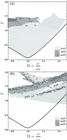
num-ber mT is therefore obtained with m = Tb/(2nπ). In
Fig. 6.a, we show the different states nx1T , whereas in Fig. 6.b , we display the results for nx2T . These two distinct phase diagrams explain the bistability observed in experiments in the central zone of the phase diagram (Fig. 4). The disagreement between the prediction for the threshold condition (10) and the numerics is related to our way to define the Poincar´e section, assuming that the ball is detached when separated from the membrane by a distance of 5% of the position of the membrane. The existence of a synchronized region with a period 2T below the critical curve (see Fig. 6.b for Ω ∼ 1.4) is due to our method for obtaining (10), i.e a detachment criteria is not strong enough to predict an established regime. Nevertheless, the superposition of the two phase diagrams allows to qualitatively recover the different sta-ble zones observed experimentally.
(b) 2.0 0.8 1.0 1.2 1.4 0.0 0.5 1.0 1.5 1x1T 2x1T nx1T (a) 2.0 Γ 0.8 1.0 1.2 1.4 0.0 0.5 1.0 1.5 1x2T 2x2T nx2T Γ Ω = ω ω0 Ω = ω ω0
FIG. 6: Numerical phase diagrams for the bouncing behav-iors of (a) nx1T and (b) nx2T states. The regions in black correspond to n = 1, in dark gray to n = 2 and in light gray to n > 4.
IV. CONCLUSION
To conclude, we will firstly recall the main result of this study: the value of the frequency and the related effects of the support deformations strongly influence the
differ-ent thresholds between the dynamical states and allow to stabilize states that are not usual for the BB system. Similar dynamical states such as the 1x2T may be ob-served for bouncing droplets. Our theoretical approach which captures the essential physics of a ball bouncing on a vibrating membrane can provide insights on the vi-brating droplet experiments [7–9]. As mentioned ear-lier, an analogy between the bouncing of a ball on an elastic membrane and of a drop on a fluid bath can be made. In our case, the new elastic degree of freedom, as compared to the (BB) system, is due to the membrane deformations while in the droplet experiments it comes from the liquid surface tension. The main difference is that there is a large energy dissipation due to the lubri-cation of the air film between a drop and a surface, so that the parameter βecan no longer be neglected. As a
consequence a transition point exists at which the curve giving the bouncing threshold becomes monotonously in-creasing. This transition arises when βi = 2−β
2 e
2βe . Above
this threshold, there is a single minimum at w = 0 while below it, two extrema are present at Ω = 0 and Ω = Ω∗.
The frequency Ω∗ is the resonant frequency of the drop
(or the membrane) shifted by the effect of energy dissipa-tion. This transition has been recently illustrated [8]. In that work, the authors measure the bouncing threshold for drops with different viscosities. When the dissipa-tion within the drop is large enough, the minimum of the curve Γc(ω) disappears. The same trend was observed
by Couder et al. [7] using a silicon oil with a large vis-cosity. In the case of bouncing on a fluid bath, we can therefore expect a peculiar motion of the drop, different from the one observed when the drop is in a 2x1T dy-namical state [12]. Finally, it is important to stress that our model could particularly be applied to the case of a drop bouncing on a soap film [9]. In this recent work, the authors have not explored the effect of the vibrat-ing frequency. A similar behavior to the one observed in our study should be recovered. We hope that this study will motivate future experimental investigations on these different bouncing systems.
We would like to thank federation Doeblin (CNRS, FR2800) for financial support.
[1] E. Fermi, Phys. Rev. 75, 1169 (1949). [2] P. Pieranski, J. Phys. 44, 573 (1983).
[3] N. B. Tufillaro, T. M. Mello, Y. M. Choi, and A. M. Albano, J. Phys. 47, 1477 (1986).
[4] J. Guckenheimer, P. Holmes, Nonlinear Oscillations, Dy-namical Systems, and Bifurcations of Vector Fields, Ap-plied Mathematical Sciences, Vol. 42, Springer-Verlag, New York, 1983.
[5] P. Coullet and C. Tresser, J. Phys. C 539, C5-25 (1978). [6] M. Feigenbaum, J. Stat. Phys, 19, 25 (1978).
[7] Y. Couder, E. Fort, C.H. Gautier, and A. Boudaoud,
Phys. Rev. Lett. 94, 17780 (2005).
[8] T. Gilet, D. Terwagne, N. Vandewalle, and S. Dorbolo, Phys. Rev. Lett. 100, 167802 (2008).
[9] T. Gilet and J. W. M. Bush, Phys. Rev. Lett. 102, 14501 (2009).
[10] J. A. Greenwood, K. L. Johnson, S-H Choi and M. K. Chaudhury, J. Phys. D: Appl. Phys. 42, 035301 (2009). [11] M. Henon, Physica D, 5, 412 (1982).
[12] S. Proti`ere, A. Bouadoud and Y. Couder J. Fluid. Mech 554, 85 (2006).