Supercritical transition to turbulence in an inertially-driven von Karman closed flow

HAL Id: hal-00118719

https://hal.archives-ouvertes.fr/hal-00118719v3

Submitted on 22 Jan 2008

HAL is a multi-disciplinary open access

archive for the deposit and dissemination of

sci-entific research documents, whether they are

pub-lished or not. The documents may come from

teaching and research institutions in France or

abroad, or from public or private research centers.

L’archive ouverte pluridisciplinaire HAL, est

destinée au dépôt et à la diffusion de documents

scientifiques de niveau recherche, publiés ou non,

émanant des établissements d’enseignement et de

recherche français ou étrangers, des laboratoires

publics ou privés.

inertially-driven von Karman closed flow

Florent Ravelet, Arnaud Chiffaudel, François Daviaud

To cite this version:

Florent Ravelet, Arnaud Chiffaudel, François Daviaud. Supercritical transition to turbulence in an

inertially-driven von Karman closed flow. Journal of Fluid Mechanics, Cambridge University Press

(CUP), 2008, 601, pp.339-364. �hal-00118719v3�

hal-00118719, version 3 - 22 Jan 2008

closed flow.

Florent Ravelet,1, 2 Arnaud Chiffaudel,1and Fran¸cois Daviaud1

1_{Service de Physique de l’Etat Condens´e, Direction des Sciences de la Mati`ere, CEA-Saclay, CNRS URA 2464,}

91191 Gif-sur-Yvette cedex, France

2_{Present address: Laboratory for Aero and Hydrodynamics, Leeghwaterstraat 21, 2628 CA Delft, The Netherlands}∗

(Dated: accepted in JFM, January 18, 2008)

We study the transition from laminar flow to fully developed turbulence for an inertially-driven von K´arm´an flow between two counter-rotating large impellers fitted with curved blades over a wide range of Reynolds number (102

−106). The transition is driven by the destabilisation of the azimuthal shear-layer, i.e., Kelvin–Helmholtz instability which exhibits travelling/drifting waves, modulated travelling waves and chaos below the emergence of a turbulent spectrum. A local quantity —the energy of the velocity fluctuations at a given point— and a global quantity —the applied torque— are used to monitor the dynamics. The local quantity defines a critical Reynolds number Recfor the onset of time-dependence in the flow, and an upper threshold/crossover Ret

for the saturation of the energy cascade. The dimensionless drag coefficient, i.e., the turbulent dissipation, reaches a plateau above this finite Ret, as expected for a “Kolmogorov”-like turbulence

for Re → ∞. Our observations suggest that the transition to turbulence in this closed flow is globally supercritical: the energy of the velocity fluctuations can be considered as an order parameter characterizing the dynamics from the first laminar time-dependence up to the fully developed turbulence. Spectral analysis in temporal domain moreover reveals that almost all of the fluctuations energy is stored in time-scales one or two orders of magnitude slower than the time-scale based on impeller frequency.

PACS numbers: 47.20.-k, 47.20.Ft, 47.27.Cn,

47.27.N-I. INTRODUCTION

Hydrodynamic turbulence is a key feature for many common problems (Lesieur, 1990; Tennekes and Lumley, 1972). In a few ideal cases, exact solutions of the Navier– Stokes equations are available, based on several assump-tions such as auto-similarity, stationariness, or symmetry (for a collection of examples, see Schlichting, 1979). Un-fortunately, they are often irrelevant in practice, because they are unstable. Two of the simplest examples are the centrifugal instability of the Taylor–Couette flow be-tween two concentric cylinders, and the Rayleigh–B´enard convection between two differentially heated plates: once the amount of angular momentum or heat is too impor-tant to be carried by molecular diffusion, a more efficient convective transport arises. Increasing further the con-trol parameter in these two examples, secondary bifurca-tions occur, leading rapidly to temporal chaos, and/or to spatio-temporal chaos, then to turbulence.

Several approaches have been carried in parallel con-cerning developed turbulence, focused on statistical prop-erties of flow quantities at small scales (Frisch, 1995) or taking into account the persistence of coherent structures in a more deterministic point of view (Lesieur, 1990; Ten-nekes and Lumley, 1972). One of the major difficulty concerning a self-consistent statistical treatment of tur-bulence is indeed that it depends on the flow in which it

∗_{Electronic address: florent.ravelet@ensta.org}

takes place (for instance wakes, jets or closed flows). At finite Re, most turbulent flows could still keep in average some geometrical or topological properties of the laminar flow (for example the presence of a B´enard–von K´arm´an street in the wake of a bluff body whatever Re), which could still influence its statistical properties (La Porta et al., 2001; Ouellette et al., 2006; Zocchi et al., 1994).

Furthermore, we have recently shown in a von K´arm´an flow that a turbulent flow can exhibit multistability, first order bifurcations and can even keep traces of its history at very high Reynolds number (Ravelet et al., 2004). The observation of this turbulent bifurcation lead us to study the transition from the laminar state to turbulence in this inertially driven closed flow.

A. Overview of the von K´arm´an swirling flow

1. Instabilities of the von K´arm´an swirling flow between flat disks

The disk flow is an example where exact Navier–Stokes solutions are available. The original problem of the flow of a viscous fluid over an infinite rotating flat disk has been considered by von K´arm´an (1921). Experimentally, the problem of an infinite disk in an infinite medium is difficult to address. Addition of a second coaxial disk has been proposed by Batchelor (1951) and Stewartson (1953). A cylindrical housing to the flow can also be added. Instabilities and transitions have been extensively studied in this system (for instance in Escudier, 1984;

Gauthier et al., 1999; Gelfgat et al., 1996; Harriott and Brown, 1984; Mellor et al., 1968; Nore et al., 2005, 2004, 2003; Schouveiler et al., 2001; Sørensen and Christensen, 1995; Spohn et al., 1998). The basic principle of this flow is the following: a layer of fluid is carried near the disk by viscous friction and is thrown outwards by centrifugation. By incompressibility of the flow, fluid is pumped toward the centre of the disk. Since the review of Zandbergen and Dijkstra (1987), this family of flow is called “von K´arm´an swirling flow”. In all cases, it deals with the flow between smooth disks, at low-Reynolds numbers, enclosed or not into a cylindrical container.

2. The “French washing machine”: an inertially-driven, highly turbulent von K´arm´an swirling flow.

Experimentally, the so-called “French washing-machine” has been a basis for extensive studies of very high-Reynolds number turbulence in the last decade (Bourgoin et al., 2002; Cadot et al., 1997, 1995; Douady et al., 1991; Fauve et al., 1993; La Porta et al., 2001; Labb´e et al., 1996; Leprovost et al., 2004; Mari´e and Davi-aud, 2004; Moisy et al., 2001; Ravelet et al., 2004; Tabel-ing et al., 1996; Titon and Cadot, 2003; Zocchi et al., 1994). To reach a Kolmogorov regime in these stud-ies, a von K´arm´an flow is inertially-driven between two disks fitted with blades, at a very high-Reynolds number (105

.Re . 107

). Due to the inertial stirring, very high turbulence levels can be reached, with fluctuations up to 50% of the blades velocity, as we shall see in this article. Most of the inertially-driven von K´arm´an setups stud-ied in the past dealt with straight blades. Von K´arm´an flows with curved-blades-impellers were first designed by the VKS-team for dynamo action in liquid sodium (Bour-goin et al., 2002; Monchaux et al., 2007). With curved blades, the directions of rotation are no longer equivalent. One sign of the curvature —i.e., with the convex face of the blades forward, direction (+)— has been shown to be the most favourable to dynamo action (Mari´e et al., 2003; Monchaux et al., 2007; Ravelet et al., 2005). The turbulent bifurcation (Ravelet et al., 2004) has been ob-tained with the concave face of the blades forward, di-rection (−). In this last work, we discussed about the respective role of the turbulent fluctuations and of the changes in the mean-flow with increasing the Reynolds number on the multistability.

B. Outline of the present article

Our initial motivation to the present study was thus to get an overview of the transition to turbulence and to check the range where multistability exists. We first describe the experimental setup, the fluid properties and the measurement techniques in § II. The main data pre-sented in this article are gathered by driving our experi-ment continuously from laminar to turbulent regimes for this peculiar direction of rotation, covering a wide range

f > 0 f > 0 Rc H z r O (a) − + R (b)

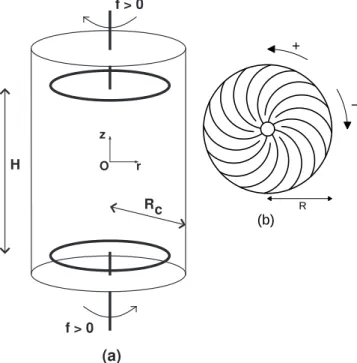
FIG. 1 (a) Sketch of the experiment. The flow volume be-tween the impellers is of height H = 1.8 Rc. (b) Impellers

used in this article. The disks radius is R = 0.925 Rc and

they are fitted with 16 curved blades: the two different direc-tions of rotation defined here are not equivalent. This model of impellers has been used in the VKS1 sodium experiment (Bourgoin et al., 2002) and is called TM60.

of Reynolds numbers. In § III and § IV we characterise the basic flow and describe the transition from the lam-inar regime to turbulence through quasi-periodicity and chaos and explore the construction of the temporal spec-trum of velocity fluctuations. The continuity and global supercriticality of the transition to turbulence is a main result of this article.

In § V we obtain complementary data by comparing the two different directions of rotation and the case with smooth disk. We show how inertial effects clearly dis-criminate both directions of rotation at high-Reynolds numbers.

We then summarize and discuss the main results in § VI.

II. EXPERIMENTAL SETUP

A. Dimensions, symmetries and control parameter

The cylinder radius and height are, respectively, Rc =

100 mm and Hc= 500 mm. A sketch of the experiment

can be found in figure 1(a). We use bladed disks to ensure inertial stirring. The impellers consist of 185 mm diame-ter stainless-steel disks each fitted with 16 curved blades, of curvature radius 50 mm and of height h = 20 mm

(fig-C µ at 15o C µ at 30o C ρ Re range 99% 1700 580 1260 50 − 2, 000 93% 590 210 1240 130 − 5, 600 85% 140 60 1220 550 − 19, 000 81% 90 41 1210 840 − 28, 000 74% 43 20 1190 1, 800 − 56, 000 0% 1.1 0.8 1000 570, 000 − 1, 200, 000 TABLE I Dynamic viscosity µ (10−3_{Pa.s) at various}

temper-atures, density ρ (kg.m−3_{) at 20}o

C and achievable Reynolds number range for various mass concentrations C of glycerol in water.

ure 1b). The distance between the inner faces of the disks is H = 180 mm, which defines a flow volume of aspect ratio H/Rc= 1.8. With the curved blades, the directions

of rotation are no longer equivalent and we can either ro-tate the impellers anticlockwise —with the convex face of the blades forward, direction (+) or clockwise (with the concave face of the blades forward, direction (−).

The impellers are driven by two independent brushless 1.8 kW motors, with speed servo loop control. The max-imal torque they can reach is 11.5 N.m. The motor ro-tation frequencies {f1 ; f2} can be varied independently

in the range 1 ≤ f ≤ 15 Hz. Below 1 Hz, the speed regulation is not efficient enough, and the dimensional quantities are measured with insufficient accuracy. We will consider for exact counter-rotating regimes f1 = f2

the imposed speed of the impellers f .

The experimental setup is thus axisymmetric and sym-metric towards rotations of π around any radial axis pass-ing through the centre O (Rπ-symmetry), and we will

consider here only Rπ-symmetric mean solutions, though

mean flows breaking this symmetry do exist for these im-pellers, at least at very high-Reynolds numbers (Ravelet et al., 2004). A detailed study of the Reynolds number dependence of the “global turbulent bifurcation” is out of the scope of the present article and will be presented else-where. Also, since we drive the impellers independently, there is always a tiny difference between f1 and f2 and

the Rπ-symmetry of the system cannot be considered as

exact. In the following, we will keep using this symme-try —very useful to describe the observed patterns– but we will keep in mind that our system is only an approxi-mation of a Rπ-symmetric system. The consequences on

the dynamics will be analysed in the discussion (§ VI.A). In the following, all lengths will be expressed in units of Rc. We also use cylindrical coordinates {r ; z} and the

origin is on the axis of the cylinder, and equidistant from the two impellers to take advantage of the Rπ-symmetry

(see figure 1a). The time unit is defined with the impeller rotation frequency f . The integral Reynolds number Re is thus defined as Re = 2πf R2

cν− 1

with ν the kinematic viscosity of the fluid.

As in previous works (Mari´e and Daviaud, 2004; Rav-elet et al., 2005, 2004), we use water at 20 − 30o

C as

working fluid to get Reynolds numbers in the range 6.3 × 104

. Re . 1.2 × 106

. To decrease Re down to laminar regimes, i.e., to a few tens, we need a fluid with a kinematic viscosity a thousand times greater than that of water. We thus use 99%-pure glycerol which kinematic viscosity is 0.95 × 10−3m2.s−1at 20oC (Hodgman, 1947)

and should be able to study the range 50 . Re . 900. To cover a wide range of Reynolds numbers and match these two extreme ranges, we then use different mixes of glyc-erol and water, at temperatures between 15 and 35o

C. The physical properties of these mixtures are given in table I, where C is the mass percentage of glycerol in the mixture. Solutions samples are controlled in a Couette viscometer.

The temperature of the working fluid is measured with a platinum thermoresistance (Pt100) mounted on the cylinder wall ({r = 1 ; z = 0}). To control this tem-perature, thermoregulated water circulates in two heat exchangers placed behind the impellers. Plexiglas disks can be mounted between the impellers and heat exchang-ers to reduce the drag of the impellexchang-ers-back-side flows. They are at typically 50 mm from the impellers back sides. However, these disks reduce the thermal coupling: they are used in turbulent water flows and taken away at low Reynolds number.

B. Experimental tools, dimensionless measured quantities and experimental errors

Several techniques have been used in parallel: flow visualisations with light sheets and air bubbles, torque measurements and velocity measurements.

Flow visualisations are made in vertical planes illumi-nated by approximately 2 mm thick light sheets. We look at two different positions with respect to the flow: either the central meridian plane where the visualised compo-nents are the radial and axial ones or in a plane almost tangent to the cylinder wall where the azimuthal compo-nent dominates. Tiny air bubbles (less than 1 mm) are used as tracing particles.

Torques are measured as an image of the current con-sumption in the motors given by the servo drives and have been calibrated by calorimetry. Brushless motors are known to generate electromagnetic noise, due to the Pulse-Width-Modulation supply. We use armoured ca-bles and three-phase sinusoidal output filters (Schaffner FN5010-8-99), and the motors are enclosed in Faraday cages, which enhances the quality of the measurements. The minimal torques we measured are above 0.3 N.m, and we estimate the error in the measurements to be ±0.1 N.m. The torques T will be presented in the di-mensionless form:

Kp= T (ρR5c(2πf ) 2

)−1

Velocity fields are measured by Laser Doppler Ve-locimetry (LDV). We use a single component DAN-TEC device, with a He–Ne Flowlite Laser (wave length

632.8 nm) and a BSA57N20 Enhanced Burst Spectrum Analyser. The geometry of the experiment allows us to measure in one point either the axial component Vz(t)

or the azimuthal component Vθ(t). Though the

time-averaged velocity field V is not a solution of the Navier-Stokes equations, it is a solenoidal vector field, and it is axisymmetric. We thus use the incompressibility condi-tion ∇ · V = 0 to compute the remaining radial compo-nent Vr.

The measurements of the time-averaged velocity field are performed on a {r ×z} = 11×17 grid, using a weight-ing of velocities by the particles transit time, to get rid of velocity biases as explained by Buchhave et al. (1979). This acquisition mode does not have a constant sition rate, so we use a different method for the acqui-sition of well-sampled signals to perform temporal anal-ysis at single points. In this so-called dead-time mode, we ensure an average data rate of approximately 5 kHz, and the Burst Spectrum Analyser takes one sample ev-ery single millisecond such that the final data rate is 1 kHz. For practical reasons, this method is well-suited for points close to the cylindrical wall, so we choose the point {r = 0.9 ; z = 0} for the measurements in fig-ures 3, 4 and 5. The signals are re-sampled at 300Hz by a “Sample And Hold” algorithm (Buchhave et al., 1979). Let us now consider the experimental error on the Reynolds number value. The speed servo-loop control ensures a precision of 0.5% on f , and an absolute pre-cision of ±0.002 on the relative difference of the im-pellers speeds (f1− f2)/(f1+ f2). The main error on the

Reynolds number is thus a systematic error that comes from the estimation of the viscosity. As far as the vari-ation of the viscosity with temperature is about 4% for 1o

C and the variation with concentration is about 5% for 1% of mass concentration, we estimate the absolute error on Re to ±10% (the temperature is known within 1o

C). However, the experimental reproducibility of the Reynolds number is much higher than ±10%. In the range 100 . Re . 500 we are able to impose Re within ±5.

III. FROM ORDER TO TURBULENCE: DESCRIPTION OF THE REGIMES

This section describes the evolution of the flow from the laminar regime to the fully developed turbulence, i.e., for 30 . Re . 1.2 × 106

. This wide-range study has been carried for the negative sense of rotation (−) of the propellers.

A. Basic state at very low Reynolds number

At very low-Reynolds number, the basic laminar flow respects the symmetries of the problem. It is stationary, axisymmetric and Rπ-symmetric. This state is stable at

Re = 90, where we present a flow visualisation in fig-ure 2(a-b). In figfig-ure 2(a), the light sheet passes through

the axis of the cylinder. The visualised velocities are the radial and axial components. The poloidal part of the flow consists of two toric recirculation cells, with axial pumping directed to the impellers.

The flow is also made of two counter-rotating cells, separated by an azimuthal flat shear-layer, which can be seen in figure 2(b) where the light sheet is quasi-tangent to the cylinder wall. Both the azimuthal and axial com-ponent vanishes in the plane z = 0 which is consistent with the axisymmetry and the Rπ-symmetry. This flat

shear-layer is sketched in figure 2(e). A LDV velocity field is presented in section V (figure 10c-d).

B. First instability – stationary bifurcation

The first instability for this flow has been determined by visualisation and occurs at Re = 175 ± 5 for both di-rections of rotation. The bifurcation is supercritical, non-hysteretic, and leads to a stationary regime, with an az-imuthal modulation of m = 2 wave number. We present a visualisation of this secondary state in figure 2(c), at Re = 185. The axisymmetry is broken: one can see the m = 2 modulation of the shear-layer, also sketched in fig-ure 2(e). One can also note that Rπ-symmetry is partly

broken: the bifurcated flow is Rπ-symmetric with respect

to two orthogonal radial axis only. This first instability is very similar to the Kelvin–Helmholtz instability. (Nore et al., 2003) made a proper theoretical extension of the Kelvin–Helmholtz instability in a cylinder. Their model is based on the use of local shear-layer thicknesses and Reynolds numbers to take into account the radial varia-tions in the cylindrical case.

We observe this m = 2 shear-layer to rotate very slowly in a given direction with a period 7500f−1_{. This}

cor-responds to a very low frequency, always smaller than the maximum measured dissymmetry of the speed servo loop control between both independent motors (§ II.B). This is probably the limit of the symmetry of our sys-tem, i.e., the pattern is at rest in the slowly rotating frame where both frequencies are strictly equal (see dis-cussion in § VI.A). For convenience, we will describe the dynamics in this frame.

The laminar m = 2 stationary shear-layer pattern is observed up to typically Re ≃ 300 where time-dependence arises.

To investigate the time-dependent regimes, we now also perform precise velocity measurements at a given point in the shear-layer. We measure the azimuthal com-ponent vθ at {r = 0.9 ; z = 0}, using the dead-time

acquisition mode (see § II).

Below, we describe and illustrate the observed dynam-ics and the building-up of the chaotic and turbulent spec-tra. The next section IV is complementary: we quantita-tively characterize the transitions as much as we can, we discuss the mechanisms and we finally propose a global supercritical view of the transition to turbulence.

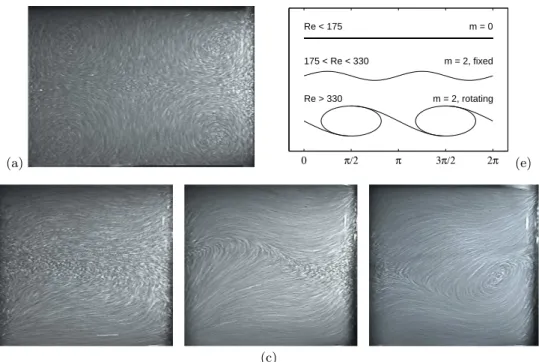
(a) 0 π/2 π 3π/2 2π m = 0 m = 2, fixed m = 2, rotating Re < 175 175 < Re < 330 Re > 330 (e) (b) (c) (d)

FIG. 2 Visualisation and schematics of the basic laminar flow for impellers rotating in direction (−). The lightning is made with a vertical light sheet. Pictures are integrated over 1/25 s with a video camera, and small air bubbles are used as tracers. Picture height is H −2h = 1.4Rc. Laminar axisymmetric flow at Re = 90, meridian view (a). Views in a plane near the cylinder

wall at Re = 90 (b), Re = 185 (c) and Re = 345 (d). The development of the first m = 2 instabilities —steady undulation (c) and rotating vortices (d)— is clearly visible on the shape of the shear-layer. We give sketches of the shear-layer for these Reynolds numbers in (e).

C. From drifting patterns to chaos

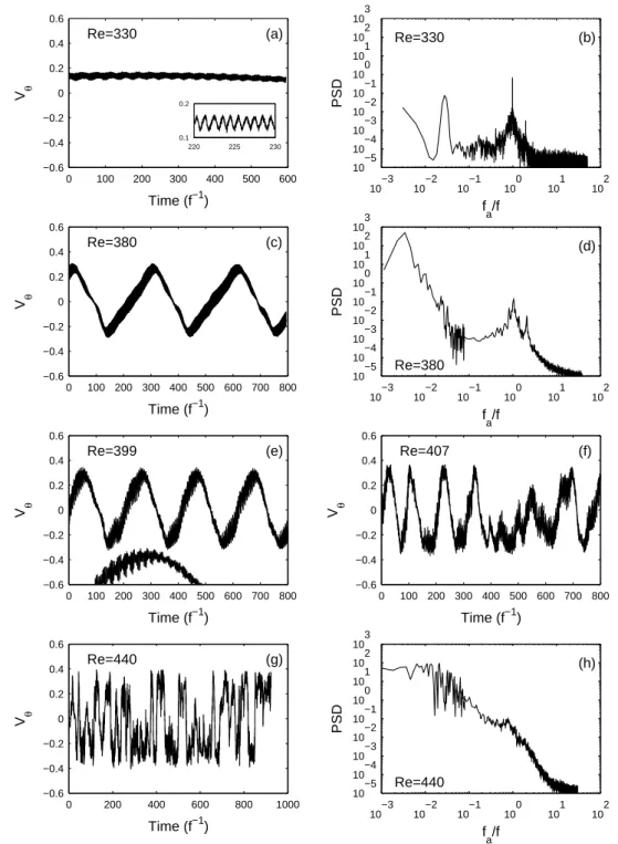
We present time series of the velocity and power spec-tral densities at five Reynolds numbers in figure 3: Re = 330 ± 5, Re = 380 ± 5, Re = 399 ± 5, Re = 408 ± 5 and Re = 440 ± 5.

1. Oscillation at impeller frequency

The point at Re = 330 ± 5 is the first point where a clear temporal dynamics is observed: a sharp peak in the spectrum (figure 3b) is present at the impeller rotation frequency fa = f —emphasized in the Inset of figure 3(a).

This oscillation exists for higher Re with the same small amplitude: it is too fast to be explicitly visible on the long time series of figure 3, but it is responsible for the large width of the signal line.

In comparison, a similar measurement performed at Re ≃ 260 reveals a flat signal with a very low flat-spectrum with just a tiny peak —1/1000 of the amplitude measured at Re = 330— at fa= f and we have no data

in-between to check an evolution.

On the spectra, we observe the first harmonic, but never shows the expected blade frequency 8f nor a mul-tiple. So, it is not clear if it corresponds to the basic fluid instability mode or just to a small precessing mode due to the misaligning of the impeller axis or even to mechanical

vibrations transmitted to the fluid through the bearings. Since the travelling-wave mode of the next paragraph is much stronger and richer in dynamics we will consider that the signal at fa= f is a “minor” phenomenon, i.e.,

a perturbation of the steady m = 2 mode.

In figure 3(a) the mean velocity is not zero, but around vθ= +0.17 during the 600 time units of acquisition, i.e.,

during 600 disks rotations. This value of the velocity has no special meaning and depends on the phase be-tween the fixed measurement point and the slowly drift-ing shear-layer (§ III.B). The measurement point indeed stays on the same side of the shear-layer for this time-series but, on much longer time scales, we measure the m = 2 shear-layer rotation typical period.

Further observation on signal and spectrum of fig-ure 3a-b reveals some energy at low frequency around fa≃ f /30, corresponding to slowly relaxing modulations:

the slowness of this relaxation is the clear signature of the proximity of a critical point.

2. Drifting/Travelling Waves

For 330 < Re < 389 the velocity signal is periodic with a low frequency fD. This is illustrated at Re = 380 in

figure 3(c-d). The mean velocity is now zero: the shear-layer rotates slowly such that the measurement point is alternatively in the cell rotating with the upper impeller

0 100 200 300 400 500 600 −0.6 −0.4 −0.2 0 0.2 0.4 0.6 (a) V θ Time (f−1) Re=330 220 225 230 0.1 0.2 10−3 10−2 10−1 100 101 102 10−5 10−4 10−3 10−2 10−1 100 101 102 103 (b) f a/f Re=330 PSD 0 100 200 300 400 500 600 700 800 −0.6 −0.4 −0.2 0 0.2 0.4 0.6 (c) V θ Time (f−1) Re=380 10−3 10−2 10−1 100 101 102 10−5 10−4 10−3 10−2 10−1 100 101 102 103 (d) f a/f Re=380 PSD 0 100 200 300 400 500 600 700 800 −0.6 −0.4 −0.2 0 0.2 0.4 0.6 (e) V θ Time (f−1) Re=399 0 100 200 300 400 500 600 700 800 −0.6 −0.4 −0.2 0 0.2 0.4 0.6 (f) V θ Time (f−1) Re=407 0 200 400 600 800 1000 −0.6 −0.4 −0.2 0 0.2 0.4 0.6 (g) V θ Time (f−1) Re=440 10−3 10−2 10−1 100 101 102 10−5 10−4 10−3 10−2 10−1 100 101 102 103 (h) f a/f Re=440 PSD

FIG. 3 Temporal signals vθ(t) measured by LDV at {r = 0.9 ; z = 0} and power spectral densities (PSD), at: (a-b) Re = 330,

(c-d) Re = 380, (e) Re = 399 , (f) Re = 408 and (g-h) Re = 440. fa is the analysis frequency whereas f is the impellers

rotation frequency. Inset in (a): zoom over the fast oscillation at frequency f . In (e), a small part of the signal is presented with time magnification (×4) and arbitrary shift to highlight the modulation at 6.2f−1_{. Power spectra are computed by the}

Welch periodogram method twice: with a very long window to catch the slow temporal dynamics and with a shorter window to reduce fast scales noise.

(vθ> 0) and in the cell rotating with the lower impeller

(vθ < 0). Visualisations confirm that this corresponds

to a travelling wave (TW) or a drifting pattern and also show that the m = 2 shear-layer is now composed of two

vortices (figure 2d) and thus deserves the name “mixing-layer”. Along the equatorial line, one notice that the parity is broken or the vortices are tilted (Coullet and Iooss, 1990; Knobloch, 1996). The velocity varies

be-tween −0.3 . vθ . 0.3. The drift is still slow but one

order of magnitude faster than the drift described above for the “steady” m = 2 pattern: one can see two peri-ods during 600 time units, i.e., fD= f /300 which is very

difficult to resolve by spectral analysis owing to the short-ness of the signal (cf. caption of figure 3). At Re = 380 (figure 3c-d), the peak at the rotation frequency is still present, but starts to spread and becomes broadband. The power spectral density at frequencies higher than 3f decreases extremely rapidly to the noise level. Let us note that Rπ-symmetry remains only with respect to

a pair of orthogonal radial axis which rotates with the propagating wave.

3. Modulated Travelling Waves

For 389 < Re < 408 the signal reveals quasiperiodic-ity, i.e., modulated travelling waves (MTW), shown in figure 3e-f at Re = 399 and 408. The MTW are regular, i.e., strictly quasiperiodic below Re = 400 and irregular above. The modulation frequency —see magnified (×4) piece of signal in figure 3e— is fM = f /(6.2 ± 0.2)

what-ever Re, even above Re = 400. It is much faster than the drift frequency (fD ∼ f /200) and seems to be

re-lated to oscillations of the mixing-layer vortex cores on the movies.

4. Chaotic regime

The upper limit of the regular dynamics is precisely and reproducibly Re = 400 and there is no hysteresis. From the visualisations, we observe that the m = 2 sym-metry is now broken. The mixing-layer vortices, which are still globally rotating around the cell in the previous direction, also behave more and more erratically with increasing Re: their individual dynamics includes excur-sions in the opposite direction as well as towards one or the other impeller. The velocity signal also looses its regularity (see figure 3e-g).

When this disordered regime is well established, e.g. for Re = 440 (figure 3g), it can be described as series of almost random and fast jumps from one side to the other side of the v = 0 axis. The peaks reached by the veloc-ity are now in the range −0.4 . vθ .0.4. The spectral

analysis of the signal at Re = 440 (figure 3h), does not re-veal any well-defined frequency peak any more. However, a continuum of highly-energetic fluctuations at low fre-quency, below fa= f and down to fa= f /100, emerges.

A small bump at the rotation frequency f is still visible, and a region of fast fluctuations above the injection fre-quency also seems to arise. Although we did not carried detailed Poincar´e analysis or equivalent and cannot char-acterize clearly a scenario, we find this transition and this regime typical enough to call it “chaos” (see also IV.B).

D. From chaos to turbulence: building a continuous spectrum

Increasing further the Reynolds number, one obtains the situation depicted in figure 4. The time-spectrum is now continuous but still evolving. We describe the two parts, below and above the impellers frequency f .

1. Slow time scales

The slow dynamics which has already been described at Re = 440 (figure 3g,h) could be thought as depending only on the largest spatial scales of the flow. It is well built above Re ≃ 103

(figure 3b). The mean velocities corresponding to each side of the mixing layer are of the order of ±0.6 at Re = 1.0 × 103

and above (figures 4a, c and g). The power spectral density below the injection frequency seems to behave with a f−1 _{power-law over}

two decades (see discussion § VI.B) for all these Reynolds numbers (figure 4). The spectral density saturates below 10−2f .

2. Fast time scales

However, the fast time scales, usually interpreted as a trace of small spatial scales fluctuations, evolve between Re = 1.0 × 103

and Re = 6.5 × 103

. At the former Reynolds number, there are few fast fluctuations decay-ing much faster than f−5/3 (figure 4(b)) and the

inter-mittent changeovers are easy to identify in the temporal signal in figure 4(a). If Reynolds number is increased, the fast (small scales) fluctuations get bigger and big-ger and behave as a power law over a growing frequency range (figure 4e, f, h). The measured slope is of order of −1.55 over 1.5 decade, i.e., 10% lower than the classical f−5/3. This value of the exponent could be ascribed to

the so-called “bottleneck” effect (Falkovich, 1994) and is compatible with the values given by Lohse and M¨ uller-Groeling (1995) (−1.56 ± 0.01) for a Taylor-micro-scale Reynolds number Rλ ≃ 100, which is an estimation for

our flow based on the results of Zocchi et al. (1994).

IV. QUANTITATIVE CHARACTERIZATION OF THE TRANSITIONS

The various dynamic states encountered have been de-scribed and illustrated in the previous section. Now, we wish to analyse some characteristic measurements — the amplitude of the velocity fluctuations and their main frequencies—, extract thresholds and critical behaviours and then address the question of the nature of the re-ported transitions.

0 100 200 300 400 500 600 700 800 −1.2 −0.8 −0.4 0 0.4 0.8 1.2 (a) V θ Time (f−1) 10 −3 10−2 10−1 100 101 102 10−4 10−3 10−2 10−1 100 101 102 103 (b) f a/f Re=1000 PSD 0 200 400 600 800 −1.2 −0.8 −0.4 0 0.4 0.8 1.2 (c) V θ Time (f−1) 10 −3 10−2 10−1 100 101 102 10−4 10−3 10−2 10−1 100 101 102 103 (d) f a/f Re=1700 PSD 10−3 10−2 10−1 100 101 102 10−4 10−3 10−2 10−1 100 101 102 103 (e) f a/f Re=2700 PSD 10−3 10−2 10−1 100 101 102 10−4 10−3 10−2 10−1 100 101 102 103 (f) f a/f Re=3800 PSD 0 200 400 600 800 1000 1200 −1.2 −0.8 −0.4 0 0.4 0.8 1.2 V θ Time (f−1) (g) 10−3 10−2 10−1 100 101 102 10−4 10−3 10−2 10−1 100 101 102 103 (h) f a/f Re=6500 PSD

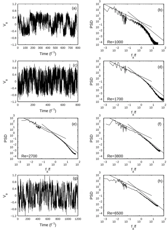
FIG. 4 (a-b): Temporal signal vθ(t) measured by LDV at {r = 0.9 ; z = 0} and power spectral density at Re = 1.0 × 103.

(c-d): Temporal signal and power spectral density at Re = 1.7 × 103

. (e-f): Power spectral densities at 2.7 × 103

and 3.8 × 103

. (g-h): Temporal signal and power spectral density at 6.5 × 103

. Solid lines in the power spectra plots are power-law eye-guides of slope −1 and −5/3. Spectra are computed as explained in the caption of figure 3.

A. From order to turbulence: a global supercriticality It is known that fully turbulent von K´arm´an flow can generate velocity fluctuations of typically 50% of the driving impellers velocity. So, we compute the variance v2

θ rms of the LDV-time-series versus the Reynolds

num-ber. This quantity is homogeneous to a kinetic energy and may be referred to as the azimuthal kinetic energy fluctuations in the mixing layer. With this method, we consider altogether the broadband frequency response of the signal. The results are reported in figure 5 for all the measurements performed between 260 . Re . 6500.

Ex-0 1000 3000 5000 7000 0 0.1 0.2 0.3 Re c Ret V θ 2 rms Re

FIG. 5 Variance of vθ(t) measured at {r = 0.9 ; z = 0}

vs. Re. Solid line: non-linear fit of the form v2

θ rms = a ×

(Re − Rec)1/2, fitted between Re = 350 and Re = 2500.

The regression coefficient is R2

= 0.990, and the fit gives Rec= 328 ± 8 with 95% confidence interval. The intersection

between this fit and the asymptotic value v2

θ rms≃ 0.27 gives

Ret= 3.3 × 103.

cept at time-dependence threshold, this quantity behaves very smoothly: it can be fitted between Re = 350 and Re = 2500 with a law in the square root of the distance to a threshold Rec≃ 330 (figure 5):

v2

θ rms∝ (Re − Rec)1/2.

Since we will show below that Rec is precisely the

threshold for time-dependence, we can make here the hypothesis that v2

θ rms is a global order parameter for

the transition to turbulence, i.e., for the transition from steady flow to turbulent flow taken as a whole. With this point of view the transition is globally supercritical.

B. Transitions from order to chaos

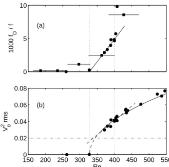
We now turn to the very first steps of the transition to time dependence. We monitor the main frequencies of the mixing layer dynamics in the TW- and MTW-regimes (see § III.C). In these regimes, even if only few periods are monitored along single time-series, we carefully es-timate the period by measuring the time delay between crossings of the v = 0 axis. These value are reported in figure 6(a) with circles. In an equivalent way, the peri-odicity of the travelling of the mixing-layer vortices on the visualisations give complementary data, represented by squares on the same figure.

1. Onset of time-dependence

The drift frequency fDof the travelling waves behaves

linearly with Re above a threshold ReT W very close to

330. Both measurement methods agree even if the visual-isations deserves large error bars in Re at least due to the shortness of our records and to a poorer thermal control.

0 5 10 1000 f D / f (a) 1500 200 250 300 350 400 450 500 550 0.02 0.04 0.06 0.08 Re V θ 2 rms (b)

FIG. 6 (a) Low-frequency fD of the quasi-periodic regime of

velocity vθ(t) measured at {r = 0.9 ; z = 0} (circles) and

drift frequency of the m = 2 shear-layer pattern from flow visualisations (squares with high horizontal error bars due to poorer temperature control). The solid line is a linear fit of fD

between the two thresholds ReT W = 330 and Rechaos= 400,

indicated by vertical dotted lines. (b) Zoom of figure 5. The dashed line is a linear fit of the lowest data between Re = 350 and Re = 450. Close to the threshold, it crosses the dash-dotted line which corresponds to the velocity due to the drift and estimates the level of imperfection.

So, the fit is made on velocity data only. We observe some level of imperfection in the quasi-periodic bifurca-tion, due to the pre-existing slow drift below ReT W: we

always observe the mixing-layer to start rotating in the sense of the initial drift.

We show in figure 6(b) a zoom of figure 5, i.e., the amplitude of the kinetic energy fluctuations. We observe that both quadratic amplitude fit and linear frequency fit converge to exactly the same threshold ReT W = Rec =

328. We can conclude that the low-frequency mode at fa = fD bifurcates at Re = 330 ± 5 through a

zero-frequency bifurcation for fD.

The question is thus how the amplitude precisely be-haves at onset. There is obviously a lack of data in the narrow range 300 . Re . 350 (figure 6(b)). It is due to the high temperature dependence of the viscosity in this regime (Reynolds varied quite fast even with thermal control) and to some data loss at the time of experimen-tal runs. Despite this lack, we present these observations because of the consistency of the different types of data —visualisations, LDV, torques— over the wide Reynolds number range. The horizontal line v2

θ rms = 0.02 in

fig-ure 6(b) corresponds to an amplitude of typically 0.15 for vθ, which is produced just by the initial shear-layer

is in good agreement with a linear extrapolation over the lower range of figure 6(b) and thus again with an imper-fect bifurcation due to the drift. If we reduce the drift by better motor frequencies matching, the onset value of vθ

will depend on the longitude of the probe location and the parabola of figure 6(b) could perhaps be observed on the m = 2 shear-layer nodes.

2. Transition to chaos

The transition to chaos is very sharply observed for Re > Rechaos= 400. There is no hysteresis. Just above

the chaotic threshold in the MTW regime (figure 3f), the signal sometimes exhibits a few almost-quasi-periodic oscillations still allowing us to measure a characteristic frequency. The measured values have been also plotted on figure 6(a) and are clearly above the linear fit. This could reveal a vanishing time scale, i.e., a precursor for the very sharp positive/negative jumps of vθ reported in

the chaotic and turbulent regimes.

We do not clearly observe any evidence of mode locking between the present frequencies which are in the progres-sion f /200 → f /6.2 → f and there is no trace of sub-harmonic cascade on any of each. This could be linked to a three-frequency scenario `a la Ruelle–Takens (Man-neville, 1990).

C. Transition to full turbulence 1. Torque data

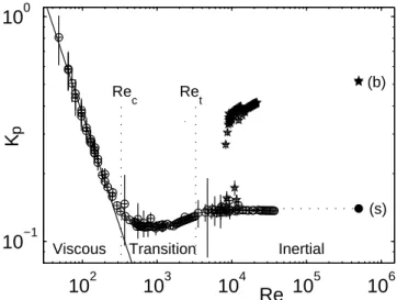
Complementary to the local velocity data, information can be collected on spatially integrated energetic data, i.e., on torque measurements Kp(Re) (figure 7). The

low-Reynolds viscous part will be described below (§ V) as well as the high-torque bifurcated branch (§ IV.D). In the high-Reynolds number regimes, the torque reaches an absolute minimum for Re ≃ 1000 and becomes inde-pendent of Re above 3300.

2. From chaos to turbulence

Is there a way to quantitatively characterize the tran-sition or the crossover between chaos and turbulence? It seems to be no evidence of any special sign to discrimi-nate between the two regimes. An empirical criterion we could propose would be the completeness of the (fa/f )−1

low-frequency part of the spectrum, clearly achieved for Re = 1000 (figure 4b). This region also corresponds to the minimum of the Kp(Re) curve (figure 7). One can

propose that below this Reynolds number, the power in-jected at the impeller rotation frequency mainly excites low frequencies belonging to the “chaotic” spectrum, whereas above Re ≃ 1000 it also drives the high frequen-cies through the Kolmogorov-Richardson energy cascade.

10

10

10

10

10

10

10

Re

K

Viscous Transition Inertial

FIG. 7 Dimensionless torque Kp vs. Re in a log-log scale

for the negative sense of rotation (−) of the impellers. The main data (◦) corresponds to the symmetric (s)-flow regime described in this part of the article. For completeness, the high-torque branch (⋆) for Re & 104

corresponds to the (b)-flow regime (Ravelet et al., 2004), i.e., to the “turbulent bi-furcation” (see § IV.D). Since both motors do not deliver the same torque in this Rπ-symmetry broken (b)-flow, the

aver-age of both values is plotted. Relative error on Re is ±10% ; absolute error of ±0.1 N.m on the torque. Rec and Ret are

the transition values computed from the fits of figure 5. The single points, displayed at Re = 5 × 105

, correspond to mea-surements in water, where Kp is extracted from a fit of the

dimensional torque in a + b × f2

for 2 × 105

.Re . 9 × 105

(Ravelet et al., 2005).

3. Inertial turbulence

The (Re − Rec)1/2behaviour can be fitted through the

quasi-periodic and chaotic regimes, up to Re ∼ 3000. Here, the azimuthal kinetic energy fluctuations level sat-urates at v2

θ rms ≃ 0.27, i.e., fluctuations of velocities at

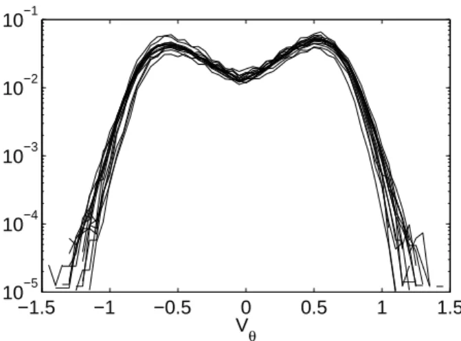
this point of the mixing-layer are of the order of 50% of the impeller tip speed. This saturation is also revealed by the Probability Density Functions (PDF) of vθpresented

in figure 8. These PDF are computed for 16 Reynolds numbers in the range 2.5 × 103

. Re . 6.5 × 103

. One can notice the bimodal character of the PDF: the two bumps, which are symmetric, correspond to the two counter-rotating cells. Furthermore, all these PDF col-lapse and are therefore almost independent of Re in this range. This is also consistent with the spectral data of figure 4(b-d) where the (fa/f )−1 slowest time-scales

re-gions which contain most of the energy —below f — ap-pear similar for Re = 1.0 × 103

and above (figure 4). The crossover Reynolds number Retat which the kinetic

energy of fluctuations saturates in figure 5 is estimated by taking the intersection of the horizontal asymptote with the fit: Ret = 3.3 × 103. This value corresponds

precisely to the value where the asymptotic plateau is reached in the Kp vs. Re diagram (figure 7). In such

−1.5 −1 −0.5 0 0.5 1 1.5 10−5 10−4 10−3 10−2 10−1 V_θ

FIG. 8 Probability density function (PDF) of vθ for 16

Reynolds numbers in the range 2.5 × 103

.Re . 6.5 × 103

.

an inertially-driven turbulent flow, the bulk dissipation is much stronger than the dissipation in boundary layers and the global dimensionless quantities thus do not de-pend on the Reynolds number past a turbulent threshold (Cadot et al., 1997; Lathrop et al., 1992).

D. Higher-Reynolds number: multistability and turbulent bifurcation

From all the above reported observations in the nega-tive direction of rotation, we conclude that the transition to turbulence is completed at Retand that the azimuthal

kinetic energy fluctuation can be considered as an order parameter for the global transition, from the onset of time-dependence Rec = 330 to the fully turbulent state

transition/crossover at Ret= 3.3×103, i.e., over a decade

in Reynolds number.

In the inertial regime above Ret, the von K´arm´an flow

driven by high-curvature bladed impellers rotating in the negative direction presents another original behaviour: Ravelet et al. (2004) have shown that the turbulent von K´arm´an flow can exhibit multistability at high-Reynolds number. To study and analyse this phenomenon, it is necessary to introduce an additional parameter with re-spect to the present paper study: the rotation velocity difference ∆f = f2− f1between the two impellers. The

so-called “Turbulent bifurcation” and multistability are observed exclusively for the negative direction of rota-tion. So, the ∆f = 0 regime presented along this paper —called (s) for symmetric in Ravelet et al. (2004)— can be observed only if both motors are started together, i.e., if ∆f is kept equal to zero at any time. Once some ve-locity difference is applied long enough —depending of the magnitude of |∆f |—, the flow changes abruptly to a one cell flow with axial pumping towards one of the im-pellers only instead of towards each impeller. This new flow —called (b) for bifurcated in Ravelet et al. (2004)—

strongly breaks the Rπ-symmetry, has no middle

shear-layer and requires much higher torque from the motors: typically 3 times the value of (s)-flow, with a finite differ-ence between the two motors. The mean reduced torque at ∆f = 0 is plotted with stars in figure 7: branches (s) and (b) co-exist for Re & Rem = 104. To recover

the Rπ-symmetric flow, one should stop the motors or at

least decrease Re below Rem.

It is worth noting that this multistability is only ob-served above Ret, i.e., for flows with a well developed

turbulent inertial Kolmogorov cascade. Furthermore, cy-cles in the parameter plane {Kp2− Kp1; f2− f1} have

been made for various Re between 100 and 3 × 105

(Rav-elet, 2005). At low-Reynolds numbers —Re . 800—, this cycle is reduced to a continuous, monotonic and re-versible line in the parameter plane. The first apparition of “topological” transformations of this simple line into multiples discontinuous branches of a more complex cy-cle is reported at Re ≃ 5 × 103

, in the neighbourhood of the transitional Reynolds number Ret, and

multista-bility for ∆f = 0 is first observed for Re ∼ 104

. The extensive study of this turbulent bifurcation with vary-ing Re is worth a complete article and will be reported elsewhere.

From the above preliminary report of our results, we emphasize the fact that the turbulent bifurcation seems really specific of fully developed turbulent flows. Whereas the exact counter-rotating flow (∆f = 0) will never bifurcate (Ravelet et al., 2004), for a small ∆f (0 < |∆f |/f ≪ 1) this turbulent bifurcation around Rem= 104 will correspond to a first order transition on

the way to infinite Reynolds number dynamics: this flow really appears as an ideal prototype of an ideal system undergoing a succession of well-defined transitions on the way from order to high-Reynolds-number turbulence.

E. The regimes: a summary

The next section concerns some aspects specific to the inertial stirring. Thereafter is the discussion (§ VI) about the role of the symmetries and of the spatial scales of the flow which can be read almost independently. The fol-lowing summary of the observed regimes and transitions is given as a support for the discussion.

• Re < 175 : m = 0, axisymmetric, Rπ-symmetric

steady basic flow (§ III.A),

• 175 < Re < 330 : m = 2, discretely Rπ-symmetric

steady flow (§ III.B),

• 330 < Re < 389 : m = 2, non Rπ-symmetric, equatorial-parity-broken travelling

waves (§ III.C.2, § IV.B.1),

• 389 < Re < 400 : modulated travelling waves (§ III.C.3),

• 400 < Re < 408 : chaotic modulated travelling waves (§ III.C.3),

• 400 < Re . 1000 : chaotic flow (§ III.C.4, § IV.B.2),

• 1000 . Re . 3300 : transition to turbulence (§ III.D, § IV.C.2),

• Re & 3300 : inertially-driven fully turbulent flow (§ IV.C.3),

• Re & 104

: multivalued inertial turbulence regimes (§ IV.D).

V. VISCOUS STIRRING VS. INERTIAL STIRRING We now focus on the specificities of the inertial stir-ring. In the preceding parts, a single rotation sense, the negative (−), was studied. However, very relevant infor-mation can be obtained from the comparison of data in both senses of impellers rotation, which is equivalent to have two sets of impellers with opposite curvature at any time in the same experiment.

The guideline for this analysis is the global energetic measurements along the whole Reynolds number range. The data for sense (−) have already been partly dis-cussed in the preceding part (figure 7), but the full set comes here in figure 9. At low Reynolds number the two curves are identical, which means that the blades have no effect on the viscous stirring. This is analysed in § V.A. However, at high Reynolds number, there is a factor 3 between both curves, denoting very different inertial regimes, as discussed in § V.B.

A. From viscous to inertial stirring

While Re . 300, the dimensionless torque Kpscales as

Re−1. We are in the laminar regime (Schlichting, 1979)

and the viscous terms are dominant in the momentum balance. These regimes correspond to m = 0 or m = 2 steady flows, with an eventual slow drift (§ III.A & III.B). From the power consumption point of view, both di-rections of rotations are equivalent. The two curves — circles for direction (−) and left triangles for direction (+)— collapse for Re . 300 on a single curve of equa-tion Kp= 36.9Re−1.

We performed velocity field measurements for the two flows at Re ≃ 120 − 130 (figure 10c-f). The differences between the two directions are minor. The order of mag-nitude of the mean poloidal and toroidal velocities are the same within 15% for both directions of rotation in the laminar regime, whereas at very high Re, they strongly differ (by a factor 2) (Ravelet et al., 2005).

The flow is thus not sensitive to the shape of the im-peller blades in the laminar regime. To explain this, we make the hypothesis that for these large impellers of ra-dius 0.925Rc, fitted with blades of height h = 0.2Rc,

the flow at low Re is equivalent to the flow between flat disks in an effective aspect ratio Γ = (H − 2h)/Rc= 1.4.

Nore et al. (2004) numerically studied the flow between counter-rotating smooth flat disks enclosed in a cylinder and report the dependence of the first unstable mode wave number on the aspect ratio Γ = H/Rc. In their

computations, the critical wave number is m = 1 for Γ = 1.8, whereas for Γ = 1.4, it is m = 2 as we do observe in our experiments.

We thus compare in figure 10 our experimental veloc-ity fields to a numerical simulation performed by Caroline Nore at the same Re and in aspect ratio Γ = 1.4. The three fields are very close. A possible physical explana-tion for this effect is the presence of viscous boundary layers along the resting cylinder wall. The typical length scale of the boundary layer thickness can be estimated as δ = Re−1/2. At the Reynolds number when the

im-pellers blades start to become visible, i.e., at Re ≃ 300, this boundary layer thickness is of the order of δ ≃ 6 mm, while the gap between the impellers and the cylinder wall is 7.5 mm. It is also of the order of magnitude of the min-imum distance between two blades. For Re . 300, the fluid is thus kept between the blades and can not be ex-pelled radially: it rotates solidly with the impellers. The stirring cannot be considered as inertial and does not depend on the blades shape.

For Re & 300, the dimensionless torque starts to shift from a Re−1 law and simultaneously discriminates

tween both sense of rotation: the inertial stirring be-comes dominant over the viscous stirring. Simultane-ously also, the steady flow becomes unstable with respect to time-dependence (§ III and IV ).

B. Inertial effects

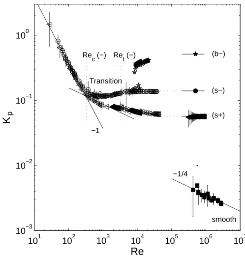
At high Reynolds number, we observe in figure 9 dif-ferent behaviours for Kpin both sense of rotation. Sense

(−) passes a minimum for Re ≃ 1000 and then rapidly reaches a flat plateau above Ret = 3300 (see § IV.C),

whereas sense (+) asymptotically reaches a regime with only a third of the power dissipation of sense (−). To-gether with the curved blade data, figure 9 presents addi-tional data for smooth disks. The dimensionless torque Kp is approximately 30 times smaller for smooth disks

than for bladed disks, and does not display any plateau at high-Reynolds number but a Re−1/4 scaling law, as

described by Cadot et al. (1997).

It is tempting to compare our curve Kp(Re) with the

classical work of Nikuradse (1932, 1933) consisting in a complete and careful experimental data set about the turbulence in a pipe flow with controlled wall rough-ness. The data concern the friction factor —equivalent of Kp— measured over a wide range between Re = 500

and Re = 106

, which is shown to strongly depend of the wall roughness above Re ≃ 3000. The wall roughness is made by controlled sand grains of diameter in the range 1/507 to 1/15 of the pipe radius, somewhat smaller than our blades height h/Rc = 1/5 which can be thought as

10

10

10

10

10

10

10

10

10

10

10

Re

K

FIG. 9 Compilation of the dimensionless torque Kp vs. Re for various flows. All data stands for Rπ-symmetric von-K´arm´an

flows except the branch labelled (b−) (⋆): see caption of figure 7 for details. (◦) : direction of rotation (−). (⊳) : direction of rotation (+); the solid line is a non-linear fit of equation Kp= 36.9 × Re−1between Re = 30 and Re = 250. Some data for flat

disks of standard machine shop roughness, operated in pure water up to 25Hz (squares) are also displayed with a Re−1/4 _fit.

Another −1/4 power law is fitted for the positive direction of rotation for 330 ≤ Re ≤ 1500 and is displayed between Re = 102

and Re = 104

. Relative error on Re is ±10% ; absolute error of ±0.1 N.m on the torque. Recand Retare the transition values

computed from the fits of figure 5.

This data set has defied theory along decades and still motivates papers. Recently, Goldenfeld (2006) and Gioia and Chakraborty (2006) proposed phenomenologi-cal interpretations and empiriphenomenologi-cal reduction of Nikuradse’s data. In few words, both recent works connect the very high-Reynolds inertial behaviour —a plateau at a value which scales with the roughness to the power 1/3— to the Blasius Re−1/4 law for the dissipative region at

in-termediate Re. Goldenfeld (2006), using a method from critical point physics, finds a scaling for the whole domain above Re ≃ 3000, whereas Gioia and Chakraborty (2006) describe the friction factor over the same Reynolds range according to Kolmogorov’s phenomenological model.

Compared with pipe flow results and models, our Kp(Re)-curve (figure 9) looks very similar except for the

region Gioia and Chakraborty (2006) called the energetic regime. Indeed, in our specific case the basic flow itself is already dominated by vortices of the size of the vessel.

The negative direction (circles in figure 9) shows a min-imum followed by a plateau above Ret= 3300 and is in

agreement with the general inertial behaviour described above. However for the positive direction (left triangles in figure 9), the Kp curve seems continuously decreasing

up to Re ≃ 106

. Looking closer, one can observe a short Re−1/4 Blasius regime for Re between 300 and 1500 —

highlighted by a fit in figure 9— followed by a very slow variation over the next two decades: logarithmic correc-tions are still visible in the range 104

.Re . 5×104

. For this direction it is more difficult to define a threshold for the plateau observed in pure water (Mari´e, 2003). Nev-ertheless, this threshold should be of order of 105

, i.e., much higher than with negative rotation.

A possible explanation of this strong difference may rely in the structure of the flow inside the impellers, i.e., in-between the blades. Let us first assume that this flow is dominated by what happens along the extrados of the

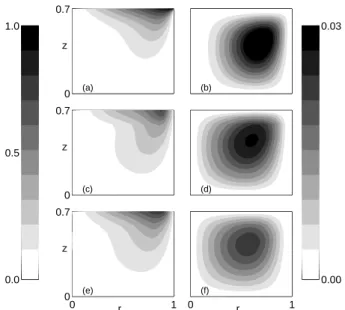
0 0.7 z (a) (b) 0 0.7 z (c) (d) 0 1 0 0.7 z r (e) 0 _r 1 (f) 0.0 0.5 1.0 0.00 0.03

FIG. 10 Comparison between a numerical simulation (a-b) performed with the code of Nore et al. (2003) in a cylinder of aspect ratio Γ = 1.4 at Re = 120 and two experimental velocity fields measured by LDV in direction (+) at Re = 130 (c-d) and in direction (−) at Re = 120 (e-f). The flow quanti-ties which we present are in (a-c-e) the azimuthal velocity vθ

and in (b-d-f) the poloidal stream function Ψ. Presenting the fields between 0 ≤ r ≤ 1 and 0 ≤ z ≤ 0.7 is sufficient due to axisymmetry and Rπ-symmetry. Blades or smooth disk are

at z = 0.7.

blades, on which the pressure is the higher. Then we can assume that the blades curvature leads to stable bound-ary layers in positive rotation and to Goertler instabil-ity in negative rotation. The first case develops Blasius boundary layers, whereas the latter develops turbulent boundary layers with much more vortices. Therefore, when the boundary layer detaches —somewhere along the blades or at least at their end— the Blasius boundary layer in the positive rotation sheds less turbulent vortices than the Goertler’s unstable layer does in the negative rotation.

The above description can be sufficient to explain why the negative rotation is able to produce a Kolmogorov cascade even at quite low-Reynolds numbers near Ret.

However if, in the positive rotation case, the flow is only seeded by vortices produced by the stable boundary layer which develops along the smooth blade faces, it is clear that a Blasius Re−1/4 can be observed in this

transi-tion Reynolds range and that a full inertial regime does not occur below a very high-Reynolds number owing to the very small roughness of the blades faces. This could be why both curves in figure 9 look so different: the lower one looks qualitatively like a low-roughness bound-ary flow and the upper one looks like a high-roughness boundary flow. Anyway, this may only account for a part of the flow driving: the resistive torque is much higher for any bladed impellers than for flat disks as shown in

figure 9.

Our observation of the closed von K´arm´an turbulent flow is thus consistent with the claim by Goldenfeld (2006) that full understanding of turbulence requires ex-plicit accounting for boundary roughness.

VI. DISCUSSION AND CONCLUSION A. Symmetries and first bifurcations

As for many flows, the similarity of the flow behaviour at low Reynolds number with intermediate-size non-linear system is obvious: breaking a spatial symmetry first, then a temporal symmetry and finally transit to chaos by a quasi-periodic scenario.

Comparable study has been carried both experimen-tally and numerically in the von K´arm´an flow with flat disk and variable aspect ratio by Nore et al. (2005, 2004, 2003). Our results agree well with their results on the first instability mode m = 2 if considering the fluid in the blade region as almost solidly driven, which reduces the aspect ratio (see § V.A). However, all thresholds ap-pear at much lower Re for bladed impellers than for flat disks: 175 vs. 300 for the first steady bifurcation and 330 vs. above 600 for the first temporal instability of m = 2 mode, not observed in Nore et al. (2005) study.

Another important difference between both system concerns its symmetries. Whereas Nore and collabora-tors deal with exact counter rotation by using a single motor to drive both disks, our experimental setup uses two independent motors and reaches only a approxima-tion on a counter-rotating regime. As a consequence, the Rπ-symmetry is stricto sensu broken at any Reynolds

number and the group of symmetry of our problem is SO(2) instead of O(2). To evaluate the level of symmetry breaking we can use a small parameter (Chossat, 1993; Porter and Knobloch, 2005), e.g. ǫ = (f1− f2)/(f1+ f2)

which is between 10−4 and 10−3in our runs.

Carefully controlling this parameter is an interesting issue: recently, in almost the same von K´arm´an flow in the positive sense of rotation at high Re, de la Torre and Burguete (2007) reported bistability and a turbulent bifurcation at exactly ǫ = 0 between two Rπ-symmetric

flows. For non-zero ǫ, the mixing layer lies slightly above or below the equator and it randomly jumps between these two symmetric positions when ǫ is carefully set to zero.

With our very small experimental ǫ, we verify theo-retical predictions (Chossat, 1993; Porter and Knobloch, 2005) for the 1:2 spatial resonance or k − 2k interaction mechanism with slightly broken reflexion symmetry. In-stead of mixed mode, pure mode and heteroclinic cycles —specific of O(2) and carefully reported by Nore et al. (2005, 2004, 2003)— we only observe drifting instability patterns, i.e., travelling waves and modulated travelling waves, characteristic of SO(2). Also, the drift frequency is very close to zero at the threshold Rec = 330

(fig-ure 6a), in agreement with the prediction fD ∼ O(ǫ)

(Chossat, 1993; Porter and Knobloch, 2005). This bi-furcation to travelling waves is similar to the 1-D drift instability of steady patterns, observed in many systems (see, e.g. Fauve et al., 1991). It relies on the breaking of the parity (θ → −θ) of the pattern (Coullet and Iooss, 1990): the travelling-wave pattern is a pair of tilted vor-tices. The bifurcation is an imperfect pitchfork (Porter and Knobloch, 2005).

Finally, the comparison can be extended to the travel-ling waves observed with flat disks above the mixed and pure modes (Nore et al., 2005, 2003). The observed wave frequencies are of the same order of magnitude in both case, which let us believe that the same kind of hydro-dynamics is involved , i.e., the blades play again a minor role at these low Reynolds numbers. However, the fre-quency ratio between the basic waves (TW) and their modulations (MTW) at onset is much higher (∼ 32) in our experiment than in the numerical simulations (∼ 5) (Nore et al., 2003). This could be due to the high number of blades.

We also wish to consider the symmetry of the von K´arm´an flow with respect to the rotation axis. In fact, the time-averaged flow is exactly axisymmetric while the instantaneous flow is not, because of the presence of blades. However, axisymmetry can be considered as an effective property at any time at low-Reynolds number and at least up to Re = 175, since we have shown that the blades have almost no effect on the flow (see § V.A). With increasing Re, the blades start playing their role and effectively break the axisymmetry of the instanta-neous flow.

Finally, we emphasize that the observations made be-low Re ∼ 400 closely remind the route to chaos trough successive symmetry break for low degree of freedom dy-namical systems. Our system can thus be considered as a small system —in fact this is coherent with the aspect ratio which is of order of 1— until the Reynolds number becomes high enough to excite small dynamical scales in the flow.

B. The three scales of the von K´arm´an flow

The observations reported in this article — visualisations, spectra— evidenced three different scales. In particular, spectra contain two time-frequency domains above and below the injection frequency fa = f . Let us first make a rough sketch

of the correspondence between temporal and spatial frequency scales of the whole flow:

• the smallest space-frequencies, at the scale of the vessel, describe the basic swirling flow due to the impeller and produce the intermediate frequency-range, i.e., the peak at fa = f in the

time-spectrum;

• the intermediate space-frequencies due to the

shear-layer main instabilities produce the lowest time-frequencies;

• the highest space-frequencies produce, of course, the highest temporal frequencies, i.e., the Kol-mogorov region.

The Taylor’s hypothesis is based on a linear mapping between space- and time-frequencies. It is probably valid for the high part of the spectrum, but the mapping might be not linear and even not monotonic for the low part. We discuss each part of the spectrum in the two following paragraphs.

1. The 1/f low-frequency spectrum

Once chaos is reached at Re = 400, a strong continu-ous and monotonic low-frequency spectrum is generated (Fig. 3h). In the chaotic regime below Re ∼ 1000, the spectrum evolves to a neat −1 power law. Then, this part of the spectrum does not evolve any more with Re. Low-frequency −1 exponents in spectra are common and could be due to a variety of physical phenomena: so-called “1/f noises” have been widely studied,e.g., in the condensed matter field (see for instance Dutta and Horn, 1981).

For turbulent von K´arm´an flows driven by two counter-rotating impellers, this low time-scale dynamics has been already observed over at least a decade in liquid helium by Zocchi et al. (1994) as well as for the magnetic induc-tion spectrum in liquid metals (Bourgoin et al., 2002; Volk et al., 2006). However, experiments carried on a one-cell flow —without turbulent mixing-layer— did not show this behaviour (Mari´e, 2003; Ravelet, 2005; Ravelet et al., 2004). We therefore conclude that the 1/fa-spectrum is related to the chaotic wandering of the

mixing-layer which statistically restores the axisymme-try. Once again, the mixing-layer slow dynamics domi-nates the whole dynamics of our system, from momentum transfer (Mari´e and Daviaud, 2004) to the very high level of turbulent fluctuations (Fig. 5 and 8).

Furthermore, we can make the hypothesis that the −1 slope is due to the distribution of persistence times in each side of the bimodal distribution (Fig. 8): the low-frequency part of the spectrum can be reproduced by a random binary signal. Similar ideas for the low-frequency spectral construction are proposed for the magnetic in-duction in the von K´arm´an sodium (VKS) experiment (Ravelet et al., 2007). In both cases, longer statistics would be needed to confirm this idea.

2. The turbulent fluctuations

We above emphasize how the flow transits from chaos to turbulence between Re ≃ 1000 and Ret = 3300. We

label this region “transition to turbulence” and observe the growth of a power-law region in the time-spectra for

fa > f . Does this slope trace back the Kolmogorov

cas-cade in the space-spectra?

As the classical Taylor hypothesis cannot apply to our full range spectrum, we follow the Local Taylor Hypothe-sis idea (Pinton and Labb´e, 1994) for the high-frequency part fa > f . Whereas Pinton and Labb´e (1994) did not

apply their technique —using instantaneous velocity in-stead of a constant advection— to the extreme case of zero advection, we think it can be applied here owing to the shape of the azimuthal velocity PDF (figure 8). These distributions show first that the instantaneous zero veloc-ity is a quite rare event: a local minimum of the curve. The modulus of velocity spends typically 75% of the time between 1/2Vmand 3/2Vm, where ±Vmare the positions

of the PDF maxima. The sign of the advection has no effect on the reconstructed wave number. We can thus conclude that frequency and wave number modulus can be matched each other at first order by a factor equal to the most probable velocity |Vm| or by the mean of |vθ|,

both very close to each other. This approach is coherent with a binary view of the local turbulent signal jump-ing randomly between two opposite mean values, just as in turbulent flow reversal model of, e.g., Benzi (2005). Then, the high-frequency part of the spectrum is equiv-alent to the spectrum obtained by averaging the spectra of every single time-series between jumps, while the low-frequency part is dominated by dynamics of the jumps themselves.

Owing to these arguments, we are convinced that an algebraic region dominates the high-frequency part of k-spectra above Ret. Observed exponents (−1.55) are of

the order of the Kolmogorov exponent, less than 10% smaller in absolute value. Similar exponents are also en-countered at other locations in the vessel.

C. Conclusion and perspectives

The von K´arm´an shear-flow with inertial stirring has been used for a global study of the transition from order to turbulence. The transition scenario is consistent with a globally supercritical scenario and this system appears as a very powerful table-top prototype for such type of study. We have chosen to emphasize a global view over a wide range of Reynolds number. This allowed to make connections between informations relaying on local (ve-locities) or global quantities (torques, flow symmetries), as discussed in § V.B and VI.

1. Going further

As a perspective, it would be first interesting to in-crease the resolution of the analysis next to the differ-ent observed thresholds. It would also be worthwhile to perform the same wide-range study for the other sense of rotation (+) or another couple of impellers. Finally, these studies would enable a comparison of the inertial

effects on the turbulent dynamics at very high Reynolds number.

2. Controlling the mixing layer

Many results of the present study proceed from veloc-ity data collected in the middle of the shear-layer and we have shown that this layer and its chaotic/turbulent wan-dering can be responsible for the low frequency content of the chaotic/turbulent spectrum of the data.

With the slightly different point of view of controlling the disorder level, we have modified the dynamics of the shear-layer by adding a thin annulus located in the mid-plane of the flow (Ravelet et al., 2005). This property was recently used in the Von K´arm´an Sodium (VKS) ex-periment held at Cadarache, France and devoted to the experimental study of dynamo action in a turbulent liq-uid sodium flow. Dynamo has effectively been observed for the first time in this system with a von K´arm´an con-figuration using, among other characteristics, an annulus in the mid-plane (Monchaux et al., 2007) and is sensitive to the presence of this device. Moreover, clear evidence has been made that the mixing-layer large-scale patterns have a strong effect on the magnetic field induction at low frequency (Ravelet et al., 2007; Volk et al., 2006). Further studies of this effect in water experiments are under progress.

3. Statistical properties of the turbulence

Studies of the von K´arm´an flow currently in progress invoke both a wider range of data in space, with the use of Stereoscopic 3-components Particle Image Velocimetry (SPIV) and a wider range in Reynolds number.

Whereas the SPIV is slower than LDV and will not allow time-spectral analysis, it offers a global view of the flow and allows to characterize statistical properties of the turbulent velocity. Guided by the behaviour of the variance of the local azimuthal velocity revealed in the present article (figure 5), we expect to analyse the evo-lution of the spatio-temporal statistical properties with Re. Such study is very stimulating for theoretical ad-vances toward a statistical mechanics of the turbulence in 2D (Chavanis and Sommeria, 1998; Robert and Som-meria, 1991), quasi 2D (Bouchet and SomSom-meria, 2002; Jung et al., 2006) or axisymmetric flows (Leprovost et al., 2006; Monchaux et al., 2006).

Acknowledgments

We are particularly indebted to Vincent Padilla and C´ecile Gasquet for building up and piloting the exper-iment. We acknowledge Caroline Nore for making her simulations available, Arnaud Guet for his help on the visualisations and Fr´ed´eric Da Cruz for the viscosity mea-surements. We have benefited of very fruitful discussions