Improved quality check procedures of XBT profiles in MFS-VOS

(1)

HAL Id: hal-00298417

https://hal.archives-ouvertes.fr/hal-00298417

Submitted on 1 Sep 2006

HAL is a multi-disciplinary open access

archive for the deposit and dissemination of sci-entific research documents, whether they are pub-lished or not. The documents may come from teaching and research institutions in France or abroad, or from public or private research centers.

L’archive ouverte pluridisciplinaire HAL, est destinée au dépôt et à la diffusion de documents scientifiques de niveau recherche, publiés ou non, émanant des établissements d’enseignement et de recherche français ou étrangers, des laboratoires publics ou privés.

Improved quality check procedures of XBT profiles in

MFS-VOS

F. Reseghetti, M. Borghini, G. M. R. Manzella

To cite this version:

F. Reseghetti, M. Borghini, G. M. R. Manzella. Improved quality check procedures of XBT profiles in MFS-VOS. Ocean Science Discussions, European Geosciences Union, 2006, 3 (5), pp.1441-1480. �hal-00298417�

(2)

OSD

3, 1441–1480, 2006 XBT quality procedures in Mediterranean F. Reseghetti et al. Title Page Abstract Introduction Conclusions References Tables Figures J I J I Back Close Full Screen / Esc Printer-friendly Version

Interactive Discussion

EGU

Ocean Sci. Discuss., 3, 1441–1480, 2006 www.ocean-sci-discuss.net/3/1441/2006/ © Author(s) 2006. This work is licensed under a Creative Commons License.

Ocean Science Discussions

Papers published in Ocean Science Discussions are under open-access review for the journal Ocean Science

Improved quality check procedures of

XBT profiles in MFS-VOS

F. Reseghetti1, M. Borghini2, and G. M. R. Manzella3 1

ENEA-CLIM-MED, Forte S. Teresa – Pozzuolo di Lerici, P.O. Box 224, 19100 La Spezia, Italy

2

CNR-ISMAR, Physical Oceanography Sect., Forte S. Teresa – Pozzuolo di Lerici, Italy

3

ENEA-CLIM, Forte S. Teresa – Pozzuolo di Lerici, P.O. Box 224, 19100 La Spezia, Italy Received: 5 May 2006 – Accepted: 21 August 2006 – Published: 1 September 2006 Correspondence to: F. Reseghetti (reseghetti@santateresa.enea.it)

(3)

OSD

EGU

Abstract

Sippican T4/DB XBT profiles, collected in the framework of Mediterranean Forecast-ing System – Toward Environmental Prediction, are analysed, namely the possible influence of launching position height, ship speed and of probes’ characteristics. Com-parison of XBT vs CTD profiles have suggested some changes in quality control

pro-5

cedures and, more important, in the values of fall rate coefficients customised for the Mediterranean. The effects of these new procedures on the overall uncertainty on depth and on temperature measurements are estimated.

1 Introduction

Since the 60’s, eXpendable BathyThermographs (XBTs) were successfully adopted by

10

oceanographers as an easy way to collect temperature profiles by using commercial ships (Ship Of Opportunity Programs – SOOP). Different types of probes are available (T4, T5, T6, T7, Deep Blue, Fast Deep . . . ), the choice of which is depending on maximum ship speed and on maximum depth to be reached. Their characteristics and use are reviewed in several “Cookbooks”, e.g. Sy (1991), AODC (1999, 2001, 2002),

15

Cook and Sy (2001). In Table 1, some XBT properties based on guides produced by the manufacturer (i.e. Sippican, now Lockheed Martin Sippican – USA) are detailed.

The main and unsolved problem concerning XBT probes is the evaluation of the uncertainty on recorded temperature values and on the depth, the last one being es-timated by using a fall rate equation Z(t)=At–Bt2, where Z is the depth at the time t.

20

The fall rate coefficients (FRCs) proposed by manufacturer are both positive and de-pending on the XBT type (see Table 2). However, differences were found between computed depths and the ones measured by other oceanographic instruments, such as STDs or CTDs. Therefore, the Integrated Global Ocean Services System (IGOSS) Task Team released a Report (Hanawa et al., 1994, 1995) proposing new values for

25

(4)

OSD

EGU

– Japan), see Table 2, and a new technique for the calculation. The error in depth was estimated to be the greatest value between 2% or 5 m. The FRCs were calculated for the major world oceans, but not for the Mediterranean; furthermore, analyses on the behaviour of XBTs in the Mediterranean Sea are not available.

Reseghetti et al. (2006)1(hereafter PAPER-I) pointed out that XBTs dropped in

West-5

ern Mediterranean Sea have shown a general agreement with contemporaneous and co-located CTD casts, but some discrepancies in temperature values occur, namely at the thermocline depth, and in correspondence of deep thermal structures. Therefore, new FRCs and data analysis procedure better reproducing thermal structures were computed (see Table 2), and a new estimate of the uncertainty of the XBT

measure-10

ments was provided.

New XBT–CTD data have been collected in order to consolidate the results of PAPER-I, extend them to the entire Mediterranean and assess the influence of different factors. The paper is organised in this way: in Sect. 2 XBT and CTD data collection procedures are presented; in Sect. 3 the acquisition time for different probes, the

in-15

fluence of the launching position and of the mass of the different probe components, the results of calibration are reviewed; in Sect. 4, fall rate coefficients for the present dataset and all the available profiles are computed; in Sect. 5, improved values for the uncertainty on temperature are detailed. Finally, the results are discussed in Sect. 6.

2 Materials and methods

20

It is noteworthy to underline that values acquired by XBTs are in-situ temperatures measured in Celsius degrees (◦C). In the paper, the speed of a ship is given in knots (1 knot is equivalent to one nautical mile/hour). CTD profiles are considered the “true” representation of the temperature: the differences between CTD and XBT values are

1

Reseghetti, F., Borghini M., and Manzella, G. M. R.: Analysis of XBT data reliability in Western Mediterranean Sea, J. Atmospheric and Oceanic Technology, submitted, 2006.

(5)

OSD

EGU

assumed to reflect inaccuracies in the XBT measurements, which are released with three decimal digits, due to the mathematical processing.

2.1 CTD characteristics and its data processing

As in PAPER-I, CTD profiles were collected by using a Sea-Bird SBE 911 pl us au-tomatic profiler, calibrated before and after each cruise at NURC (NATO Undersea

5

Research Centre in La Spezia, Italy). The adopted falling speed was 1.0 ms−1. The apparatus has a 24 Hz sampling rate, with a (static) nominal accuracy of 0.001◦C on temperature, and of 0.0003 Sm−1on conductivity. Its (static) time constant is of 0.065 s for conductivity and temperature sensors (which implies a nominal spatial resolution of 0.065 m), and of 0.015 s for the pressure sensor (the spatial resolution is 0.015 m).

10

CTD profiles were processed by using standard Seabird’s software (Data Conversion, Alignment, Cell Thermal Mass, Filtering, Derivation of physical values, Bin Average and Splitting); afterwards, they were qualified with Medatlas protocols (Maillard et al., 2001). 2.2 XBT data acquisition and data processing

Sippican T4 and DB probes manufactured in 2003 and 2004 were launched in

15

September–October 2004 from R/V URANIA when the ship was motionless. The pro-cedures detailed in PAPER-I were adopted, by using the same data acquisition sys-tem (Sippican MK-12 readout card, and PC with Intel P-II 166 MHz-processor). The XBT sampling rate is 10 Hz, the instrumental sensitivity on temperature is of 0.01◦C, whereas the uncertainty estimated by the manufacturer is |δT|∼0.10◦C. Each XBT

20

probe was dropped within 480 s from a CTD cast. Geographical and temporal co-ordinates of the sampling positions for CTDs and XBTs are shown in Table 3.

The XBT data processing developed in PAPER-I (see Appendix A) was used, starting from the evaluation of the average value of the Empirical Time Constant (ETC). This is defined as the time that the system requires before it measures consecutive water

25

(6)

OSD

EGU

nominal accuracy of the probe. For the present sample, ETC=(0.3±0.1) s for both T4 and DB probes, a value as great as twice the overall time constant of the acquisition system. Consequently, the first three temperature values are eliminated from each XBT profile, and the sequence of temperature values was re-scaled by cutting 0.3 s. In other words, each temperature profile has the fourth measured value as starting

5

value. The remaining quality check (q.c.) procedures developed in PAPER-I are applied (Appendix B).

3 Data analysis and results

3.1 Acquisition time

Since April 2003, the data acquisition beyond the nominal terminal depth is the

stan-10

dard procedure for all the XBT probes dropped within Mediterranean Forecasting Sys-tem projects (namely MFSTEP). In such a way, the most part of copper wire on the probe side is used, and temperature values are recorded at depths deeper than nomi-nal. Practically, the depth in the Sippican software is set to 600 m for T4/T6 probes, to 900 or 1000 m for T7/DB probes, and to 2500 m for T5 probes.

15

The acquisition has been estimated as “good” until sharp variations toward negative (usually about –2.5◦C), or very hot (about 36◦C) values are recorded. Negative temper-atures indicate that the copper wire breaks on ship-side, and hot tempertemper-atures imply a wire break on probe-side. Following the procedure detailed in PAPER-I, Acquisition Time Intervals (ATIs) lower than the standard one (due to spikes, launch failure, etc.),

20

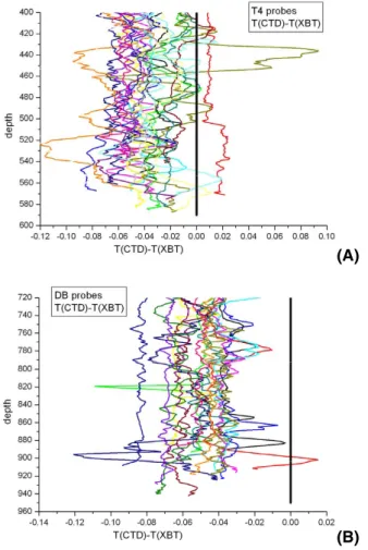
and profiles without wire breaking or a signal clearly indicating a reduced acquisition time were not included in the statistics. The comparison among XBTs with contempo-raneous and co-located CTD casts seems to exclude significant systematic effects or some unusual variations in recorded values at deeper depths (Fig. 1).

T4 probes measure temperatures warmer than CTDs (only one profile is

25

(7)

OSD

EGU

structures), but the difference is lower than ±0.12◦C. On the other hand, DB probes have warmer temperatures and four profiles show evident spikes.

If XBTs are dropped from a steady vessel, ATI can be assumed as nearly coincident with its maximum values (e.g. about 90 s for T4, and 150 s for DB probes). ATI values are practically constant when the ship speed is v ≤19 kn for T4 and v ≤16 kn for DB

5

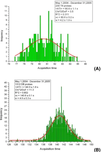
probes, whereas they decrease at higher speed, as expected. The results are shown in Table 4, and confirm the reliability of the “extended” acquisition. As an example, the ATI frequency distribution of 230 T4 probes dropped at a ship speed ranging from 21 to 27 kn (lower than the maximum nominal value) is shown in the upper plot of Fig. 2, whereas in the bottom panel the distribution for DB probes dropped since May 2004 at

10

a ship speed v ≤20 kn is plotted.

In the case of ships moving faster than the maximum value indicated by the manufac-turer, one should expect lower ATIs, and experimental results agree. From May 2004 to December 2005, 191 DB probes were launched along the transect Genova-Palermo from ships moving at v >20 kn, and their average ATI values are detailed in Table 4.

15

The number of T7 probes analysed is relatively small: 68 probes were launched from a ship having v ≤15 kn, and 15 probes from ships moving at v ∼17 kn. Their ATI values are as great as the DB ones. Few T5 probes were dropped with extended acquisition (8 XBTs), and they have shown ATI values increased at a level of about 20%, as the remaining XBT types.

20

3.2 Analysis of factors influencing the motion 3.2.1 Launching Position Height

The motion of the probes in near surface layers is supposed to be dependent on Launching Position Height (LPH) above the sea level. The manufacturer suggests LPH∼2.5 m (the available XBT Cookbooks strongly recommend LPH<15 m): in such

25

a case, the XBT ingoing vertical speed at the sea level is v ∼6.5 ms−1, as great as the A coefficient. If LPH is higher, the ingoing speed increases, and the depth computed

(8)

OSD

EGU

by software does not correspond to the real depth of the probe (such a discrepancy is more evident in the near surface layer). In addition, if LPH is higher than suggested, the probe motion in air can show a significant displacement from the vertical direction, and several probes can get in seawater in a nearly horizontal position.

In the working procedures, it is fundamental to assure that the probe reaches quickly

5

a spin rate of about 15 Hz, needed to maintain the vertical direction of the motion through the water, and the standard falling conditions. Analyses by Green (1984) and Seaver and Kuleshov (1982) show that XBT probes have the correct speed and spin values after about 1.5 s, independently on the initial launching conditions. The only ef-fect of non-standard initial launching conditions should be described by an offset term

10

(smaller than about 5 m) added to the depth computed by the software. This correc-tion can dramatically influence the reliability of measurements where strong thermal gradients occur.

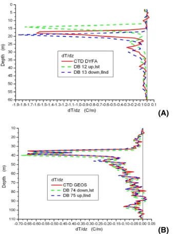
In September–October 2004, twin XBT drops were done during the same CTD cast from different positions (LPH∼2.5 m, and LPH∼8.0 m), aiming to check the influence

15

of LPH. The time delay between the drops is lower than 360 s, and differences due to internal wave should be small. The temperature gradient profiles for XBTs and CTDs are shown in Fig. 4 for T4 probes, and in Fig. 5 for DB probes. The results are ambiguous: the value of the depth at which the thermal gradient starts, as measured by XBTs, is either deeper or shallower than real, without apparent correlations with

20

LPH and time delay. 3.2.2 XBT mass

The mass of a probe is a parameter potentially influencing its motion. The manufacturer states that the weight of XBTs of the same type should vary within a range of few grams, but this could modify the motion. As remarked by Hanawa and Yoshikawa (1991), small

25

and random changes in weight can be caused by the wire technical coating process by enamel, and such a variability should influence the values of FRCs. A wire thicker than normal has less enamel, its linear density is higher, and the probe buoyancy is reduced.

(9)

OSD

EGU

Consequently, a probe falls down faster (increased A), but its weight reduction is also faster, due to an unreeling heavier wire, and a greater B coefficient is required (see PAPER-I for details).

In order to identify a possible correlation between the weight and ATI, also taking into account the ship speed, the mass (in air) of XBT probes launched along the transect

5

Genova-Palermo was measured. In detail, before the drop each probe and canister were weighted, but without the cap. The components of the canister were weighted again after the launch. In addition, the different components of some failed probes were individually weighted as well as the length of copper wire was measured. Results are shown in Tables 5 and 6. The average values of the weights are more or less

10

constant, but the individual variability is high. Unfortunately, the probes dropped in this test were not weighted: therefore, the influence of the weight on the probe motion and on FRCs is unknown.

3.3 Calibration of XBT probes & data acquisition system

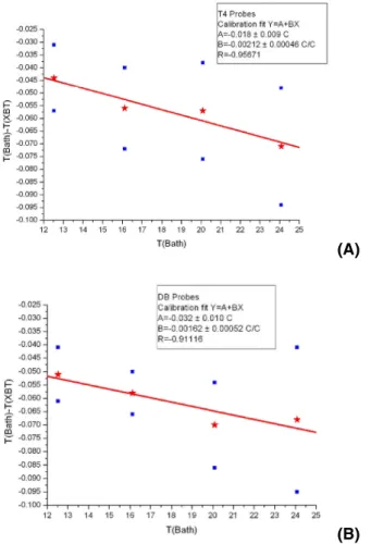
In September 2004, six T4 and six DB probes were calibrated at four reference

tem-15

peratures (12.5, 16, 20, and 24◦C). The data were recorded by using always the same acquisition system composed by a PC, Sippican MK-12 card, cable, and connection box. Each probe was immersed in the bath 10 min before the data acquisition, which was 30.0 s long. Such a procedure allows the identification of the intrinsic bias due to the thermistor and the data acquisition system.

20

For each probe the measured temperatures are always higher than the bath (from 0.04◦C to 0.08◦C), with a standard deviation of about 0.01◦C at the lower temperature, and of about 0.03◦C at higher values. Their average values (see Fig. 6) are also in agreement with independent measurements, such as MEDARGO floats, although they are not contemporaneous and co-located (Poulain, 2005)2. A linear function well

re-25

produces the temperature differences, the constant term of the function being related

2

(10)

OSD

EGU

to the total wire length, which is of about 1800 m (550 m in the probe and 1250 m in the canister) for T4, and of about 2300 m (950 m and 1350 m) for DB. The coefficients of the fit for T4 and DB probes are shown in Fig. 6: in general, they are compatible.

4 Fall rate coefficients

As pointed out in PAPER-I, the IGOSS’ FRCs reported in Table 2 did not reproduce the

5

depth of thermal structures measured by CTDs, especially in deeper layers, and the standard technique proposed in Hanawa et al. (1994, 1995) cannot be applied to the temperature profiles from Mediterranean Sea (see Fig. 7).

The procedures presented in PAPER-I (see Appendix C for details) provide the re-sults shown in Table 7. It is evident that T4 probes move slower than previously

es-10

timated. In Fig. 8, the profile of the average temperature difference between CTDs and T4 probes is plotted, with the range of variability. A comparison between T4 pro-files computed with IGOSS’ FRCs and q.c. procedures as in Manzella et al. (2003), and following the proposed technique is shown. In upper layers, the use of improved q.c. procedures strongly reduces the average temperature difference. DB probes have

15

the same behaviour as T4 (Fig. 9), but with a stronger variability in upper layers as well as in the region between 200 and 300 m depth.

In region below the nominal maximum depth, probes show a relative strong variabil-ity, due to poor sample at depth deeper than about 550 m for T4 (Fig. 8), and about 920 m for DBs (Fig. 9).

20

4.1 Fine tuning

When the profiles of the average temperature difference, ∆T=T(CTD)–T(XBT), were analysed a “systematic” shift clearly appeared, mainly at deeper depths, see Fig. 8 B for T4, and Fig. 9 B for DB probes. A better agreement is reached by introducing a correction term deriving from linear regression (function of the depth D) of temperature

(11)

OSD

EGU

differences, ∆T(D)=∆T₀+m*D. The coefficients of the function (see Table 8) were cal-culated by using ∆T values below 100 m down to 900 m for DBs, and below 100 m down to 550 m for T4 probes. The constant term for T4 and DB probes, which could be thought as a bias, is compatible with the difference in temperature deduced from the calibration, whereas the angular coefficient has a value very similar to the pressure

5

effect reported in Roemmich and Cornuelle (1987).

This correction to XBT profiles further improves the agreement (Fig. 8 for T4 and Fig. 9 for DB probes).

4.2 Analysis on complete MFS dataset

When the present XBT sample has been added to the one analysed in PAPER-I, new

10

FRCs have been computed in the way detailed in Appendix C (see results in Table 7). Then, the fine-tuning linear correction was applied again (Table 8).

In Table 9, the maximum depth of each profile calculated with different FRCs and q.c. procedures is shown. When the computed best pair of FRCs is applied to each profile, the difference in depth between CTD and XBT is not greater than 3 m along

15

the whole profile. The real depth of T4 probes is always smaller when compared with values obtained by using IGOSS FRCs and previous q.c. procedures (Manzella et al., 2003), and the difference is up to about 20 m. DB probes show smaller and more vari-able differences, but in general their true depth is deeper than previously calculated. In Fig. 10, the maximum difference observed at each reference depth is shown.

Be-20

low 300 m depth, the proposed FRCs reduce by some metres the disagreement with respect to the real depth when compared with the Hanawa et al. (1995) FRCs. As a further result, below the nominal standard depth, DB probes have a percent depth error smaller with respect to T4 probes.

In Figs. 11 and 12, a comparison is proposed between T4 and DB probes,

respec-25

tively. The average temperature difference between CTD and XBT profiles obtained by applying the q.c. procedures detailed in Manzella et al. (2003) with IGOSS’s FRCs, and all new q.c. procedures with new FRCs is shown. The discrepancies are strongly

(12)

OSD

EGU

reduced in the upper region, and the systematic effect at deeper depths (XBT values always warmer than the ones of CTD casts) disappears. The main, and usual, effect of the rescaling, due to the addition of ETC, is a reduction of the disagreement in regions where upper thermal gradient occurs. Sometimes, this correction can produce in up-per layers an even significant spike if strong and sharp gradient occurs (about 2◦Cm−1).

5

The profile of the averaged temperature difference obtained with new q.c. procedures is more or less symmetric around the null value. Some spikes remain in deeper regions due to only depth differences, usually enhanced where deep thermal structures occur. It has to be pointed out that DBs have a reduced range of variability with respect to T4 probes. In any case, temperature values recorded at depth deeper than 550 m for T4

10

and 920 m for DB probes have to be accurately analysed before their use.

5 Uncertainty on XBT measurements

The uncertainty (δT) on XBT temperature values is a very important parameter: the manufacturer indicates |δT|∼0.10◦C, but the analysed profiles seem to suggest that this value is variable and depth dependent. Therefore, a “phenomenological”

uncer-15

tainty has been estimated, taking also into account the influence of depth error on the recorded temperatures. We remind that the fine-tuning procedure practically eliminates a bias term probably correlated with the “systematic” of probe and data acquisition sys-tem, and including the differences found in the calibration. Usually, a depth error, which is enhanced where thermal structures occur, appears as a spike when the difference

20

of contemporaneous temperature measurements of CTD and XBT is plotted. Such an error can originate the main part of the temperature uncertainty.

In order to estimate the global uncertainty, the maximum depth error and the stan-dard deviation (probe-to-probe variability) deduced from calibrations have to be con-sidered. The error in depth (Fig. 10) can induce an average temperature uncertainty

25

|δT|∼0.03–0.05◦C below about 200 m depth, but can produce dramatic disagreement in upper region, where a strong thermal gradient can occur. Calibrations suggest a

(13)

OSD

EGU

standard deviation within the range |0.01–0.03|◦C. It has to be pointed out that if the results of the calibrations are combined with the other uncertainties reviewed in this paper, then |δT_tot|∼0.05–0.10◦C, in agreement with measurements based both on CTD casts (Reseghetti et al. 2006)1and on MEDARGO floats (Poulain, 2005)2.

A realistic value for the uncertainty along the profile has been experimentally

ob-5

tained by calculating the range of temperature difference at each depth. The initial step requires the identification of the thermal gradient (depth and strength) in near surface layer, and of the depth of deeper thermal structures. Unfortunately, the upper layer remains a critical region out of a defined and reliable statistical prediction.

The analysis on the complete XBT sample confirms the results obtained in PAPER-I,

10

and the final uncertainties on temperature value recorded by both Sippican T4 and DB probes can be summarized as follows:

– |δT| ≤ 0.10◦C from the surface down to thermocline, when existing;

– |δT| ≤ 0.50◦C where the thermocline starts (if any), and proportional to its strength (with some spikes up to about 3.0◦C, but over a layer not deeper than few metres);

15

– |δT| ≤ 0.07◦C below the basis of the thermocline (|δT| ≤ 0.14◦C in regions where identified thermal structures occur).

6 Comments and conclusions

In this paper, the performances of T4 and DB probes manufactured by Sippican are analysed by comparing XBT temperature profiles and contemporaneous CTD casts in

20

Western Mediterranean Sea. Other results are based on the larger MFS program. The reliability of the extended data acquisition for XBT probes has been demon-strated. ATI can be increased by about 20% without evident and significant differences in the recorded temperatures. As expected, the measured acquisition time depends on the ship speed. The launch of DB and T7 probes from ships moving faster than

(14)

OSD

EGU

nominal has been successfully done, and the quality of recorded values seems to be good along the whole profile. Therefore, the extended acquisition beyond the nominal depth can be used as a standard launching procedure without evident influence on the quality of measured values. A better reproduction of the thermal structures where gradients starts is usually obtained when the first three recorded values are excluded,

5

and the profile is rescaled by the empirical response time.

The launch of pairs of probes from different height during the same CTD cast does not clearly indicate the influence of the height of the launching position mainly on the evaluation of the right thermocline starting depth. Each probe has a random behaviour, although the sample of analysed XBTs is small.

10

The evaluation of a possible dependence of ATI values from the initial mass of the probe has been practically impossible, due to variability in weight of each component of a probe, and of the linear density of the wire.

The fall rate equation with the coefficients proposed by Hanawa et al. (1995) de-scribes the motion of XBT probes in a reasonable way, but a not negligible difference,

15

depending on the XBT type, frequently occurs. The discrepancy in depth is large for T4 probes: a good reproduction of their profiles is allowed only if the A coefficient is sig-nificantly reduced. Deeper thermal structures occur at a depth reduced with respect to the values obtained by using the previous procedures (up to about 20 m, see Table 8). On the contrary, DB probes present smaller differences.

20

The calculated B coefficients are within the range of variability allowed by IGOSS Report for each specific type. The effect of B coefficient should be enhanced by the ex-tended acquisition. This means a motion for a time longer than usual when the probes are lighter, but no significant or unusual differences appear in temperature profiles be-low the nominal terminal depth. Recorded values are reliable down to about 550 m

25

depth for T4 and about 920 m depth for DB probes.

The calibration of XBTs and data acquisition system strengthens the confidence in XBT measurements: the measured difference indicates the global good quality of the recording apparatus (within the range 0.04–0.08◦C), as well as a reduced

(15)

probe-to-OSD

EGU

probe variability (0.01–0.03◦C). In any case, all the calibrated probes measure temper-atures warmer than the real values.

The validity of the quality check procedures proposed in PAPER-I is confirmed. The analysis of the temperature difference profiles for T4 and DB probes indicates a resid-ual systematic component, whose value below 100 m depth can be well reproduced by

5

a linear function of the depth. The constant term, which should be related to the intrin-sic properties of the probe and data acquisition system, is in substantial agreement with those cited in literature, and with the calibration values. The angular coefficient seems to allow the description of the most the residual depth error and other unknown and probe-specific unpredictable effects. In such a way, the systematic difference between

10

XBTs, and CTDs or MEDARGO measurements is significantly reduced.

As a final remark, analyses on the present T4 and DB dataset indicate that, after the application of the proposed new FRCs and q.c. procedures, and “statistically speaking” (each probe is a different measurement system), XBTs produce temperature profiles in agreement with CTD measurements, with “reasonable” depth errors and uncertainties

15

(16)

OSD

EGU

Appendix A

Start-up effect on XBT data

The time constant (TC) of an XBT recording system can influence the measurements mainly in upper layers. The bridge circuit reaches equilibrium within two sampling

5

intervals (the thermistor resistance value is sampled at a constant rate of 10 Hz.), but the probe requires an interval of 4.5 TC before it detects surface seawater temperature within the instrumental accuracy. In literature, the finite response time of XBT probe thermistor is estimated at a level of 0.63 s. Therefore, the true sea temperature cannot be detected down to about 4 m depth. The magnitude of the error in temperature is

10

depending on the difference between the thermistor and the sea temperature at 4 m depth. Also a significant TC associated to the probe nose was found, and a probe-to-probe and read-out card depending on an initial transient time of about 0.1 s.

More in detail, the thermistor requires 0.15 s in order to detect the 63% of a step ther-mal signal, whereas the overall time constant (OTC) of the system is slightly greater

15

(OTC∼0.16 s). During such a time interval, the probe moves down about 1 m, and this is the depth uncertainty intrinsic to the acquisition system. A temperature change is completely detected within about 0.6 s. The analysis of the first detected temper-atures values shows some differences. As a consequences, the empirical response time (ETC) of a probe is defined as the time needed before a probe reaches the

sta-20

tionary regime in seawater. It is identified by the occurrence of three consecutive tem-perature values differing less than 0.10◦C (the nominal accuracy) within the first ten measurements. The averaged value of such time intervals is the mean response time of the available sample for XBTs of that type. If the sequence of temperature values of each XBT profile is modified by shifting the real start by ETC: τ₀=t₀+ETC ⇒ T (τ_i)=T

25

(t_i+ETC), the discrepancies between CTD and XBT values in upper layers are signif-icantly reduced. The temperature difference T(CTD)–T(XBT) is more symmetric with respect to the null value, and the start of thermal structures is better reproduced. In any

(17)

OSD

EGU

case, this is an empirical procedure that does not describe what physically happens.

Appendix B

Quality control procedures

The quality check procedures detailed in Manzella et al. (2003) have been changed

5

in order to reduce the disagreement among raw and q.c. XBT, and CTD profiles. The Gaussian filter is applied to the raw profile, which is divided in three parts, the indepen-dent variable being the time, which has fixed increment due to the 10 Hz acquisition rate:

– Upper region, from the surface to the thermocline starting point (3-point filter);

10

– Intermediate region, down to the base of thermocline (3-point filter);

– Deeper region, from the base of the thermocline down to the bottom (7-point filter).

The software identifies the starting point of the upper thermal gradient by searching for a depth where for four consecutive times the temperature difference with respect to the previous measurement is lower than –0.10◦C. In similar way, the base of the

15

thermocline is fixed where∆T>–0.10◦C for four consecutive times. Then, the despiking and 1 m reduction procedures described in Manzella et al. (2003) are applied.

The temperature values of each XBT profile from the surface down to 3 m depth are excluded from q.c. profiles, and the last three ones also.

(18)

OSD

EGU

Appendix C

Fall Rate Coefficients computation

Several temperature profiles from Mediterranean seawaters are non-monotonic and their gradient values are near to zero over large regions; consequently, the

methodol-5

ogy proposed by Hanawa et al. (1994, 1995) cannot be successfully applied to such profiles.

FRCs well reproducing the thermal structures on CTD profile have been computed by varying the FRC values within intervals depending on XBT type:

– T4: 6.400≤A≤6.750 ms−1, and 0.00180≤B≤ 0.00240 ms−2;

10

– DB: 6.600≤A ≤6.850 ms−1, and 0.00200≤B≤ 0.00260 ms−2.

The used steps were based on the request of 1 m accuracy in depth calculation: 0.005 ms−1for the A coefficient and 0.00005 ms−2for the B coefficient. For each T4/T6 probe, (71×13) profiles were computed, and (51×13) profiles for each DB probe.

For each CTD profile, six reference points below 100 m depth where thermal

struc-15

tures occur are identified by visual inspection. Obviously, the depth of selected points differs from profile-to-profile. Then, the difference between the depth measured by the CTD and that one on the computed XBT profile is calculated in correspondence of such points, and summed up. The minimum value of the sum of the depth differences indicates the best pair of FRCs for the analysed probe. The final values of FRCs are

20

obtained by calculating the average, weighting on the length of each profile. They rep-resent a compromise between faster and slower probes; therefore, some spikes remain in temperature difference profiles.

Acknowledgements. The authors acknowledge M. Astraldi (CNR-ISMAR, Physical

Oceanog-raphy Sect., La Spezia, Italy) for the extensive use of CTD profiles. This work has been carried

25

(19)

OSD

EGU

– DG Research under contract EVK3-CT-20-00075, and ADRICOSM and ADRICOSM-EXT, financially supported by Italian Ministry of Environment, Italian Ministry of Foreign Affairs, and UNESCO.

References

AODC: Guide to MK12–XBT System (Including Launching, returns and faults), Australian

5

Oceanographic Data Centre (AODC), METOC Services, 1–63, 1999.

AODC: Expendable Bathythermographs (XBT) delayed mode. Quality control manual, Aus-tralian Oceanographic Data Centre (AODC), Data Management Group, Technical Manual 1/2001, 1–24, 2001.

AODC: Marine QC. Australian Oceanographic Data Centre (AODC), Data Management Group,

10

Technical Manual 1/2002, 1–61, 2002.

Cook, S. and Sy, A.: Best guide and principles manual for the Ships Of Opportunity Program (SOOP) and EXpendable Bathythermograph (XBT) operations, Prepared for the IOC-WMO-3rd Session of the JCOMM Ship of Opportunity Implementation Panel (SOOPIP-III), 28–31 March 2000, La Jolla, California, U.S.A., 1–26, 2001.

15

Hanawa, K., Rual, P., Bailey, R., Sy, A., and Szabados, M.: Calculation of new depth equations for Expendable Bathythermographs using a temperature-error-free method (Application to Sippican/TSK T7, T6 and T4 XBTs), Intergovernmental Oceanographic Commission (IOC) Technical Series, 42, 1994.

Hanawa, K., Rual, P., Bailey, R., Sy, A., and Szabados, M.: A new depth-time equation for

20

Sippican or TSK T7, T6 and T4 expendable bathythermographs (XBT), Deep-Sea Research Part I, 42(8), 1423–1451, 1995.

Hanawa, K. and Yoshikawa Y.: Re-examination of the depth error in XBT data, J. Atmos. Oceanic Technology, 8, 422–429, 1991.

Maillard, C., Fichaut, M., and Dooley, H.: MEDAR-MEDATLAS Protocol. Part I. Exchange

for-25

mat and quality checks for observed profiles, Rap. Int. TMSI/IDM/SISMER/SIS00-084, 1–49, 2001.

Manzella, G. M. R., Scoccimarro, E., Pinardi, N., and Tonani, M.: Improved near real time data management procedures for the Mediterranean Ocean Forecasting System – Voluntary Observing Ship Program, Ann. Geophys., 21, 49–62, 2003.

(20)

OSD

EGU

Roemmich, D. and Cornuelle, B.: Digitization and calibration of the expendable bathythermo-graph, Deep-Sea Research 34, 299–307, 1987.

Sy, A.: XBT measurements. In “WOCE Operations Manual, WHP Operation and Methods”, WHPO 91-1, WOCE Report 68/91, 1–19, 1991.

(21)

OSD

EGU

Table 1. Maximum depth and acquisition time for different XBT types. The ship speed is the

maximum value indicated by manufacturers. The maximum acquisition time is also quoted; sometimes, due to different fall rate coefficients, such values are different.

XBT Ship Depth ATI Depth ATI Type Speed Sippican Sippican IGOSS IGOSS

(kn) (m) (s) (m) (s) T4 30 460 72.9 460 70.5 T5 6 1830 290.6 – – T6 15 460 72.9 460 70.5 T7 15 760 122.5 760 118.3 T10 10 200 32.1 – – T11 6 460 269.1 – – DB 20 760 122.5 760 118.3 FD 20 1000 164.2 – –

(22)

OSD

EGU

Table 2. Different values for the coefficients of the fall rate equation are compared.

Author A (ms−1) B (ms−2) Sippican 6.472 0.00216 T4/T6/T7/DB Sippican T5 6.828 0.00182 Sippican FD 6.390 0.00182 Hanawa et al., 1995 6.691 ± 0.021 0.00225 ± 0.00030 T4/T6/T7/DB Hanawa et al., 1995 6.683 ± 0.033 0.00215 ± 0.00052 Best fit T4/T6 Hanawa et al., 1995 6.701 ± 0.023 0.00238 ± 0.00016 Best fit T7/DB Reseghetti et al., 2006 6.570 ± 0.060 0.00220 ± 0.00010 Best fit T4/T6 Reseghetti et al., 2006 6.735 ± 0.045 0.00235 ± 0.00010 Best fit DB

(23)

OSD

EGU

Table 3. The co-ordinates of CTD casts and the differences (CTD–XBT) in time and position

of the present dataset. All T4 and DB probes were launched few minutes after the CTD casts from a steady vessel by selecting free maximum depth. The label D indicates a probe launched from 2.5 m over the sea level, whereas U indicates a probe dropped from 8.0 m over the sea level.

CTD Lat (◦) Lat (‘) Lon(◦) Lon (‘) Date XBT ∆Lat (‘) ∆Lon (‘) ∆Time

(dd-mm-yy) (h:m) Dmr2 43 29.98 8 59.99 19-09-04 T4-04-D –0.024 –0.000 –00:05 Dmr17 43 30.04 8 59.91 21-09-04 T4-06-U –0.001 –0.006 –00:01 Dmr22 43 30.00 8 59.99 21-09-04 T4-07-U –0.020 –0.008 –00:01 Dmr22 43 30.00 8 59.99 21-09-04 T4-09-D +0.004 –0.004 –00:07 D281 38 58.43 9 52.17 18-10-04 T4-70-D +0.004 –0.001 –00:01 D281 38 58.43 9 52.17 18-10-04 T4-71-U –0.006 –0.009 –00:07 Da10 40 00.00 12 12.34 20-10-04 T4-76-D –0.007 –0.006 –00:01 Da10 40 00.00 12 12.34 20-10-04 T4-77-U +0.007 –0.013 –00:06 Da7 41 26.70 11 08.35 22-10-04 T4-80-D –0.012 –0.015 –00:01 Da7 41 26.70 11 08.35 22-10-04 T4-81-U –0.009 –0.011 –00:06 Dmr1 43 30.03 8 59.95 19-09-04 DB-01-U +0.006 –0.007 –00:01 Dmr1 43 30.03 8 59.95 19-09-04 DB-02-D –0.026 –0.029 –00:07 D808 43 08.13 8 54.50 24-09-04 DB-10-U –0.003 –0.014 –00:01 D808 43 08.13 8 54.50 24-09-04 DB-11-D –0.052 –0.011 –00:08 Ddyfa 43 25.00 7 51.97 30-09-04 DB-12-U +0.027 –0.028 –00:01 Ddyfa 43 25.00 7 51.97 30-09-04 DB-13-D –0.011 –0.004 –00:07 D241 38 51.43 10 10.97 18-10-04 DB-72-D –0.007 –0.002 –00:01 D241 38 51.43 10 10.97 18-10-04 DB-73-U +0.008 –0.027 –00:07 Dgeos 38 54.91 13 17.98 20-10-04 DB-74-D –0.012 –0.004 –00:01 Dgeos 38 54.91 13 17.98 20-10-04 DB-75-U +0.007 +0.001 –00:07 D50 40 20.19 13 29.95 21-10-04 DB-78-D –0.014 –0.016 –00:01 D50 40 20.19 13 29.95 21-10-04 DB-79-U +0.028 –0.010 –00:08

(24)

OSD

EGU

Table 4. Average experimental values of ATI and observed range of variability for different XBT

types. The values at v≥20 kn for T4 and DB probes are based on XBTs dropped on the transect Genova-Palermo.

XBT Speed Real <ATI> th <ATI> exp No. Range Type Max (kn) Speed (kn) (s) (s) XBT (s)

T4 30 v=0 70.5 87.3±2.0 22 83.0–90.7 T4 30 21≤ v ≤ 27 70.5 80.6±1.1 230 76.8–84.9 T5 6 5 ≤ v ≤ 7 290.5 351.0±10.9 8 332.9–362.8 T7 15 v ≤ 15 118.3 142.5±2.2 8 138.6–150.9 T7 15 v=17 118.3 136.3±1.4 15 133.2–138.2 DB 20 v=0 118.3 143.9±2.4 18 139.3–148.5 DB 20 v≤20 118.3 140.9±1.8 1312 126.3–149.6 DB 20 v=21 118.3 137.6±1.9 4 136.3–140.5 DB 20 v=22 118.3 134.2±2.2 27 130.9–140.3 DB 20 v=23 118.3 127.5±2.3 35 124.3–132.8 DB 20 v=24 118.3 122.1±2.9 31 115.6–127.0 DB 20 v=25 118.3 118.0±2.3 48 113.0–123.8 DB 20 v=26 118.3 114.2±2.5 37 109.3–118.6 DB 20 v=27 118.3 111.1±1.2 9 109.8–113.5

(25)

OSD

EGU Table 5. The initial mass and the value of the remaining component for DB dropped from ships

along the transect Genova-Palermo. M1=retaining pin mass; M2=shipboard spool (without wire) – the main part of the difference seems to be due to the insulating wax; M3=plastic canister. The same characteristics for T4 probes are added for comparison.

Number Initial Mass M M1 M2 M3

(g) (g) (g) (g) DB Dec 04 1129±4 19.0±0.1 80.7±1.8 123.1±1.2 1121≤M≤1137 18.8≤M1≤19.2 78.1≤M2≤83.4 120.2≤M3≤124.8 DB Jan 05 1128±4 19.1±0.1 80.0±0.7 119.5±0.3 1123≤M≤1136 18.9≤M1≤19.3 78.8≤M2≤80.6 118.8≤M3≤120.1 DB Feb 05 1129±4 19.5±0.1 80.1±0.7 118.0±2.0 1121≤M≤1137 19.4≤M1≤19.8 79.0≤M2≤82.1 113.6≤M3≤119.6 T4 Feb 05 1099±3 19.2±0.1 81.8±1.9 121.8±0.4 1094≤M≤1104 18.9≤M1≤19.6 78.0≤M2≤85.9 121.3≤M3≤122.6

(26)

OSD

EGU Table 6. Weight (M), length (L) and linear density (λ) of the copper wire for some probes.

T4 T4 T4 T4 T5 DB DB Ship side M (g) L (m) λ (gm−1) 128. 469 1125 0.116 162. 973 1346 0.121 152. 507 1263 0.121 158. 649 1315 0.121 131. 843 1110 0.120 161. 144 1334 0.121 156. 343 1344 0.116 Probe side M (g) L(m) λ (gm−1) 63. 967 547 0.117 63. 510 526 0.121 62. 208 516 0.121 58. 518 485 0.121 249. 480 2095 0.119 112. 212 932 0.120 106. 235 916 0.116

(27)

OSD

EGU

Table 7. The values of the coefficients of fall rate equation computed by using the new proposed

technique for different datasets: TW for the data analysed in this work, P-I for the sample analysed in PAPER-I, All for the combined dataset. The “Observed Range” columns show the interval of variability of all the best pair of FRCs of each probe. The FRCs values are sufficiently stable independently on the selected dataset.

Type <A> Observed Range <B> Observed Range

ms−1 ms−1 ms−2 ms−2 T4-TW 6.565 ± 0.090 6.470 ≤ A ≤ 6.700 0.00220 ± 0.00010 0.00215 ≤ B ≤ 0.00230 T4 P-I 6.570 ± 0.060 6.440 ≤ A ≤ 6.680 0.00220 ± 0.00010 0.00215 ≤ B ≤ 0.00230 DB-TW 6.690 ± 0.060 6.610 ≤ A ≤ 6.770 0.00235 ± 0.00010 0.00225 ≤ B ≤ 0.00240 DB P-I 6.735 ± 0.045 6.665 ≤ A ≤ 6.830 0.00235 ± 0.00010 0.00220 ≤ B ≤ 0.00240 T4 All 6.570 ± 0.065 6.440 ≤ A ≤ 6.700 0.00220 ± 0.00010 0.00215 ≤ B ≤ 0.00230 DB All 6.720 ± 0.055 6.610 ≤ A ≤ 6.830 0.00235 ± 0.00010 0.00220 ≤ B ≤ 0.00240

(28)

OSD

EGU

Table 8. Coefficients of the linear function of the depth ∆T(D)=∆T₀+m*D for the present

dataset (TW), the dataset analysed in PAPER-I (P-I), and the combined sample (All). A cer-tain variability occurs in different samples. For both T4 and DB probes, the term ∆T₀ of the sample TW is very similar to the value of systematic temperature difference deduced from the calibration at T=12.5◦ C. ∆T0( ◦ C) m (◦Cm−1) T4 TW –0.039±0.002 –0.000003±0.000001 T4 P-I –0.023±0.001 –0.000024±0.000001 T4 All –0.029±0.001 –0.000016±0.000001 DB TW –0.051±0.002 –0.000008±0.000002 DB P-I –0.029±0.001 –0.000019±0.000001 DB All –0.039±0.001 –0.000014±0.000001

(29)

OSD

EGU

Table 9. The maximum depth for analysed profiles as computed by using IGOSS coefficients

and procedures as in Manzella et al. (2003) (label H95), the q.c. procedures developed in this work and the averaged FRCs (label TW), and by using the pair of FRCs for each profile (label BF). The symbol (*) indicates T6 probes. Six T4/T6 probes over 28, and ten DB probes over 27 had some troubles, and their acquisition stopped before the end of the wire. For all T4/T6 probes the depth computed by using new q.c. procedures and FRCs is lower than that one obtained by applying Manzella et al. (2003) q.c. procedures and IGOSS’ FRCs. DB probes have irregular results due to the smaller difference between IGOSS and new FRCs.

Probe T4-T6 H95 (m) BF (m) TW (m) Probe DB H95 (m) BF (m) TW(m) 1 556 555 546 1 909 920 911 2 571 569 559 2 912 931 914 3 585 569 574 3 893 892 895 4 567 561 557 4 660 670 662 5 567 554 557 5 763 759 765 6 568 562 558 6 923 929 925 7 583 568 573 7 367 370 368 8 587 563 576 8 151 153 151 9 561 549 551 9 914 920 916 10* 575 566 565 10 916 923 918 11* 541 528 531 11 145 146 146 12* 538 530 533 12 886 888 888 13* 582 575 573 13 455 458 456 14* 524 513 514 14 917 921 919 15* 428 421 420 15 924 916 926 16* 417 414 410 16 758 764 760 17* 565 548 554 17 506 500 507 18* 536 534 527 18 905 905 908 19 541 542 532 19 942 931 944 20 562 560 552 20 407 407 408 21 560 552 549 21 940 949 942 22 462 452 454 22 901 909 903 23 537 523 528 23 87 87 88 24 429 427 421 24 908 896 911 25 586 566 575 25 918 913 920 26 442 427 434 26 929 916 931 27 571 552 561 27 886 891 888 28 186 182 183 – – – –

(30)

OSD

EGU (A)

(B)

Fig. 1. Temperature difference in deeper part of each XBT profiles, below the nominal terminal

depth: (A) for T4 probes; (B) for DB probes. The depth is computed by using IGOSS coe

ffi-cients and q.c. procedures described in Manzella et al. (2003). No systematic effect due to the extended acquisition seems to be present, but only random behaviour due to individual probe

(31)

OSD

EGU (A)

(B)

Fig. 2. Frequency distribution of ATI values: in (A) for T4 probes launched along the transect

Genova-Palermo, at a speed ranging from 21 to 27 kn; in(B) for DB probes launched

dur-ing MFSTEP and other projects at v≤20 kn. Some counts at ATI=141.3 s are due to probes dropped by setting the terminal depth to 900 m.

(32)

OSD

EGU

(A) (B)

(C)

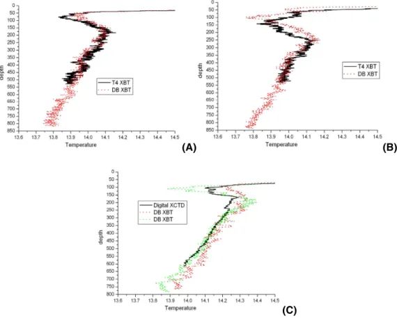
Fig. 3. Comparison among DB and T4, and XCTD measurements. Profiles are from

Genova-Palermo transect, October 2004(A–B) and September 2004 (C). In (A) and (B), DB probes

were dropped about half hour later and 13 miles distant from T4 probe. In (C), XCTD probe was dropped in the middle, the difference with respect to each DB probe being about half hour in time, and about 13 miles in distance.

(33)

OSD

EGU Fig. 4. Thermal gradient profiles in near surface layer for two pairs of T4 probes are shown.

The green dashed line always represents the former dropped probe, and the blue dashed line to the latter. For all T4 probes, the structures are well reproduced, independently on the delay in time and on the height of launching position. The plots have different scales.

(34)

OSD

EGU (A)

(B)

Fig. 5. As in Fig. 4, but for DB probes. In (A), the pair of DB probes shows an unpredictable

behaviour at the depth where thermal gradient occurs (at a level of about 2◦Cm−1). When the profile representing the temperature difference between CTD and XBTs is considered, the discrepancy is greater than 4◦C. On the other hand, the disagreement in(B) is much smaller.

(35)

OSD

EGU (A)

(B)

Fig. 6. The average values of temperature differences at each reference point (and the standard

deviation) from calibration. The values of the fit coefficients are shown in (A) for T4, and in (B) for DB probes.

(36)

OSD

EGU Fig. 7. Thermal gradient values below 150 m depth for a CTD, and a DB profile are shown. The

values are always smaller than 0.013◦Cm−1 for the CTD (green line). The range of variability for DB profile is as large as half of the previous interval: it does not allow the application of standard technique proposed by Hanawa et al. (1994, 1995). The values in red are computed by using the q.c. procedures detailed in Manzella et al. (2003); blue dotted line represents values calculated by applying all the new proposed procedures.

(37)

OSD

EGU Fig. 8. T(CTD)–T(XBT) average values for T4 probes dropped in September–October 2004.

The q.c. procedures are as in Manzella et al. (2003) (red line), and with FRCs specific of this sample with fine-tuning correction, see Table 7 (blue line).

(38)

OSD

EGU Fig. 9. As in Fig. 7, but for DB probes. Strong spikes occur at about 20 and 30 m depth, due to

(39)

OSD

EGU

Fig. 10. The experimental maximum difference in depth with respect to the corresponding CTD

profiles for T4/T6 and DB at the selected marker depth. The XBT depth is computed by using the q.c. procedures developed in the present work and new FRCs for the complete available dataset.

(40)

OSD

EGU Fig. 11. T(CTD)–T(XBT) average values for the whole sample of T4 probes. The q.c.

pro-cedures are as in Manzella et al. (2003) (red), and following this work with the fine-tuning correction quoted in Table 7 (blue). The application of all proposed q.c. procedures greatly improves the agreement between XBT and CTD profiles both in upper layers and at bottom. Data seem to be reliable down to about 550 m depth.

(41)

OSD

EGU Fig. 12. As in Fig. 11, but for all the available DB probes. The proposed new q.c. procedures

improve the agreement between XBT and CTD profiles down to about 920 m depth. Spikes remain mainly where deeper thermal structures start.