Analysis of velocity fluctuations and their intermittency properties in the surf zone using empirical mode decomposition

HAL Id: hal-00449071

https://hal.archives-ouvertes.fr/hal-00449071

HAL is a multi-disciplinary open access

archive for the deposit and dissemination of sci-entific research documents, whether they are pub-lished or not. The documents may come from

L’archive ouverte pluridisciplinaire HAL, est destinée au dépôt et à la diffusion de documents scientifiques de niveau recherche, publiés ou non, émanant des établissements d’enseignement et de

Analysis of velocity fluctuations and their intermittency

properties in the surf zone using empirical mode

decomposition

François G Schmitt, Yongxiang Huang, Zhiming Lu, Yulu Liu, Nicolas

Fernandez

To cite this version:

François G Schmitt, Yongxiang Huang, Zhiming Lu, Yulu Liu, Nicolas Fernandez. Analysis of velocity fluctuations and their intermittency properties in the surf zone using empirical mode decomposition. Journal of Marine Systems, Elsevier, 2009, 77 (4), pp.473-481. �10.1016/j.jmarsys.2008.11.012�. �hal-00449071�

Analysis of velocity fluctuations and their

intermittency properties in the surf zone

using empirical mode decomposition

Fran¸cois G. Schmitt

∗, Yongxiang Huang

, Zhiming Lu

,

Yulu Liu

Nicolas Fernandez

a_{Laboratory of Oceanography and Geosciences, CNRS UMR LOG 8187} University of Science and Technology of Lille -Lille 1

Wimereux Marine Station, 28 av. Foch, 62930 Wimereux, France b_{Shanghai Institute of Applied Mathematics and Mechanics,}

Shanghai University, 200072 Shanghai, China

Abstract

We consider here surf zone turbulence measurements, recorded in the Eastern En-glish Channel using a sonic anemometer. In order to characterize the intermittent properties of their fluctuations at many time scales, we analyze the experimental time series using the Empirical Mode Decomposition (EMD) method. The series is decomposed into a sum of modes, each one narrow-banded, and we show that some modes are associated with the energy containing wave-breaking scales, and other modes are associated with small-scale intermittent fluctuations. We use the EMD approach in association with a newly developed method based on Hilbert spectral analysis, representing the probability density function in an amplitude-frequency space. We then characterize the fluctuations in a stochastic framework using a cu-mulant generating function for all scales, and compare the results obtained from direct and classical structure function analysis, to EMD-Hilbert spectral analysis results, showing that the former method saturates at large scales, whereas the latter method is more precise in its scale approach. These results show the strength of the new EMD-hilbert spectral analysis method for data presenting a strong forcing such as found in shallow water, wave dominated situations.

Key words: Surf zone turbulence, Empirical Mode Decomposition, Intermittency, Cumulant generating function

∗ Corresponding author: Tel.: +33-321-992935; Fax.: +33-321-992901

1 Introduction

One of the main properties of fully developed turbulence is its inertial range intermittent properties, between a large-scale injection of energy and a small-scale dissipation (Frisch, 1995; Pope, 2000). In the surf zone, when waves break, the wave energy is transferred into turbulent motions through a violent, highly energetic process associated with breaking wave times scales, typically a few seconds, and then turbulence is dissipated at smaller scales (Svendsen, 1987; Battjes, 1988; Svendsen, 2005). The surf zone environment is a complex system: there are water turbulent motion at different scales, breaking waves feeding turbulence at the surface, and residual turbulence persisting from one wave to the next (Svendsen, 1987; Jaffe and Rubin, 1996). This highly ener-getic system has a strong effect on sediment transport dynamics, morpholog-ical changes associated with it, and shoreline evolution processes (Jaffe and Rubin, 1996; Cox et al., 1996; Trowbridge and Elgar, 2001; Masselink and Russell, 2006; Torres-Freyermuth et al., 2007), and also on ecological processes through influences on feeding, settlement, fertilization, bloom dynamics, etc. (Denny and Shibata, 1989; Du Preez et al., 1990; Mead and Denny, 1995).

In the intertidal zone, transport models for either sediments or living organ-isms need the description of surf zone velocity fluctuations. It is then impor-tant in this context to be able to characterize these velocity fluctuations for a wide range of scales, including highly energetic breaking waves scales and smaller turbulent scales. This is not an easy task because of the unsteadiness of breaking waves: phase-average methods are not straightworward since the wave forcing is not monochromatic; ocean breaking waves are nonlinear and present random components.

We use here for this an approach based on the Empirical Mode Decomposi-tion method which has been introduced by Huang et al. as a new time series analysis technique able to separate a given time series into a sum of modes, each one associated with well defined scales (Huang et al., 1998, 1999). This method is most efficient and interesting for nonstationary and nonlinear time series, and is efficient to separate trends from small-scale fluctuations. Due to the simplicity of its algorithm, since its introduction, the EMD method has met a large success and has been successfully applied to many topics in the natural and applied sciences: mechanical engineering (Chen et al., 2004; Loutridis, 2004), acoustics (Loutridis, 2005), meteorology and climate studies (Salisbury and Wimbush, 2002; Coughlin and Tung, 2004; J´anosi and M¨uller, 2005), and biological applications (Balocchi et al., 2004; Ponomarenko et al., 2005), among others. It has already been applied to nonstationary ocean wave data (Hwang et al., 2003; Veltcheva and Soares, 2004), but these studies focus on deep water ocean waves, which are different from surf zone breaking waves. Here we consider experimental turbulent velocity time series recorded in the

surf zone.

Sections 2 and 3 below present the methods; section 4 presents the data, and the results together with a comparison of the new method with more classical structure functions approach. Section 5 is the conclusion.

2 Empirical Mode Decomposition and Hilbert spectral analysis

2.1 The EMD algorithm

Empirical Mode Decomposition is an analysis technique which has recently been developed to study the nonlinear and nonstationary properties of time series (Huang et al., 1998, 1999) . The main idea of EMD is to locally estimate a signal as a sum of a local trend and a local detail: the local trend is a low frequency part, and the local detail a superposed high frequency. When this is done for all the oscillations composing a signal, the high frequency time series is called an Intrinsic Mode Function (IMF) and the low frequency part is called the residual. The procedure is then applied again to the residual, considered as a new times series, extracting a new IMF using a spline function, and obtaining a new residual. After the decomposition process is terminated, the EMD method expresses a time series as the sum of a finite number of IMFs and a final residual (Huang et al., 1998; Flandrin and Gon¸calv`es, 2004). The algorithm is precisely described below.

An IMF is a function that must satisfy two conditions according to the al-gorithm originally developed: (i) the difference between the number of local extrema and the number of zero-crossings must be zero or one; (ii) the run-ning mean value of the envelope defined by the local maxima and the envelope defined by the local minima is zero. The algorithm to decompose a signal into IMFs is then the following (Huang et al., 1998, 1999):

1 The local extrema of the signal x(t) are identified;

2 The local maxima are connected together by a cubic spline interpolation (other interpolations are also possible), forming an upper envelope emax(t).

The same is done for local minima, providing a lower envelope emin(t);

3 The mean is defined as m1(t) = (emax(t) + emin(t))/2;

4 The mean is subtracted from the signal, providing the local detail h1(t) =

x(t) − m1(t);

5 The component h1(t) is then considered to check if it satisfies the above

conditions to be an IMF. If yes, it is considered as the first IMF and denoted C1(t) = h1(t). It is subtracted from the original signal and the first residual,

an IMF, a procedure called “sifting process” is applied as many times as necessary to obtain an IMF. In the sifting process, h1(t) is considered as

the new data; the local extrema are estimated, lower and upper envelopes are calculated and their mean is denoted m11(t). This mean is subtracted

from h1(t), providing h11(t) = h1(t) − m11(t). Then the same procedure

starts again: it is checked if h11(t) is an IMF. If not, the sifting process is

repeated, until the component h1k(t) satisfies the IMF conditions. Then the

first IMF is C1(t) = h1k(t) and the residual r1(t) = x(t) − C1(t) is taken as

the new series in step 1.

By construction, the number of extrema decreases when going from one resid-ual to the next; the above algorithm ends when the residresid-ual has only one extrema, or is constant, and in this case no more IMF can be extracted; the complete decomposition is then achieved in a finite number of steps. The sig-nal x(t) is fisig-nally written as the sum of mode time series Ci(t) and the residual

rn(t): x(t) = N X i=1 Ci(t) + rn(t) (1)

The IMFs are orthogonal, or almost orthogonal functions (mutually uncorre-lated). This method does not require stationarity of the data and is especially suitable for nonstationary and nonlinear time series analysis (Huang et al., 1998, 1999). Numerically, it is found that each mode is localized in frequency space (Flandrin and Gon¸calv`es, 2004; Wu and Huang, 2004). EMD can be used to choose the scale truncation: it expresses the original time series as the sum of a trend (sum of modes from p to N ) and small-scale fluctuations (sum of modes from 1 to p − 1), where p is an index whose value depends on the trend decomposition which is desired.

2.2 Hilbert spectral analysis and an amplitude-frequency pdf representation

This decomposition method is a time-frequency analysis (Flandrin and Gon¸cal-v`es, 2004) since it can represent the original signal in a energy-frequency-time form at local level, using a complementary analysis technique called Hilbert-Huang spectrum (Long et al., 1995; Hilbert-Huang et al., 1998), which is presented here. Hilbert spectral analysis (HSA) (Cohen, 1995; Long et al., 1995; Huang et al., 1998) is applied to each mode, in order to locally extract a frequency and an amplitude. Each mode function Ci(t) is associated with its Hilbert

transform ˜Ci ˜ Ci(t) = 1 π Z +∞ −∞ Ci(τ ) t − τ dτ (2)

and the combination of Ci(t) and ˜Ci(t) gives the analytical signal z = Ci +

j ˜Ci = Ai(t)ejθi(t), where Ai(t) is an amplitude time series and θi(t) is the phase

the residual, the original time series is rewritten as x(t) = Re N X i=1 Ai(t)ejθi(t) (3)

For each mode, the Hilbert spectrum is defined as the square amplitude H(ω, t) = A2_{(ω, t), where ω = dθ/dt is the instantaneous frequency obtained}

using the phase information θ(t) = tan−₁ ˜

C(t)/C(t). H(ω, t) gives a local rep-resentation of energy in the time-frequency domain. The Hilbert marginal spectrum of the original time series is then written as

h(ω) = Z ∞

0 H(ω, t)dt (4)

and corresponds to an energy density at frequency ω (Long et al., 1995; Huang et al., 1998, 1999).

This can be used to define the joint probability density function (pdf) p(ω, A) of the frequency [ωi] and amplitude [Ai], which are extracted from all modes

i = 1 · · · N together. The Hilbert marginal spectrum is then rewritten as

h(ω) = Z ∞

0 p(ω, A)A

2_{dA (5)}

This definition corresponds to a second statistical moments. As introduced elsewhere (Huang et al., 2008), we then generalize Eq. (5) using arbitrary moments q ≥ 0: L(q, ω) = Z ∞ 0 p(ω, A)A q dA (6)

L(q, ω) will be used below for the computation of cumulants at a given fre-quency.

3 Characterization of intermittency using cumulants

3.1 Structure functions and cumulants

One of the characteristic features of fully developed turbulence is the inter-mittent nature of velocity fluctuations (Frisch, 1995). Intermittency provides corrections to Kolmogorov’s scaling law (Kolmogorov, 1941), which are now well established and received considerable attention in the last twenty years. Let us recall how to quantify intermittency effects on scaling laws for Eulerian isotropic turbulence. Denoting ∆Vℓ = V (x + ℓ) − V (x) the longitudinal

characterized, in the inertial range, using the scale invariant moment function ζ(q):

h|∆Vℓ|qi = Aqℓζ(q) (7)

where q > 0 is the order of moment and Aq is a constant that may depend on

q. Kolmogorov’s initial proposal, for a non-intermittent constant dissipation, leads to ζ(q) = q/3 (Kolmogorov, 1941). For intermittent turbulence, ζ(q) is proportional to a cumulant generating function, and is nonlinear and concave; only the third moment has no intermittency correction: ζ(3) = 1. The accuracy of the scaling of Eq.(7) is usually tested for each order of moment, for various values of ℓ in log-log plot, using a least-square regression (Anselmet et al., 1984). The values of ζ(q) which are then obtained may be compared and fitted to different multifractal models (among many studies, see (She and Leveque, 1994; Chen and Cao, 1995; Arneodo et al., 1996; Boratav, 1997; Schertzer et al., 1997; van de Water and Herwijer, 1999; Anselmet et al., 2001)). This way of estimating ζ(q) depends on the choice of the scaling range: one usually estimates ζ(q) for the range of scales where the exact relation ζ(3) = 1 is verified, assuming that the scaling range is the same for each order of moment.

Here there is no large sclaing range: we therefore consider another approach: instead of studying the scale dependence for each moment, we focus on the moment dependence using cumulants at a given scale. The cumulant approach has already been undertaken in the scaling turbulence framework in a few studies (see e.g. (Delour et al., 2001; Eggers et al., 2001; Chevillard et al., 2005)), where the cumulants of the cascade process (Eggers et al., 2001) or a polynomial development of the cumulant generating function (Delour et al., 2001; Chevillard et al., 2005) have been considered; see also Venugopal et al. (2006) for an application to multifractal properties of rainfall.

3.2 Non analytical cumulant generating functions

We consider here a random variable w. The cumulant generating function of its generator g = log |w| is defined as (Gardiner, 2004):

Ψ(q) = logh|w|qi (8)

The function Ψ(q) is also the second Laplace characteristic function of the generator: Ψ(q) = logheqg_{i. As a second characteristic function, it is convex}

(Feller, 1971), and can be developed using the cumulants:

Ψ(q) = ∞ X p=1 cp qp p! (9)

where cp is the pthcumulant (not to be confused with the previous Cpnotation

for mode time series). Let us recall the expression for the first cumulant:

c1 = hgi = hlog |w|i (10)

We also know that c2 = hg2i − c21, and cn depends on all moments hgpi

(1 ≤ p ≤ n). The theorem of Marcienkiewicz states that, if it exists, the development in Eq.(9) is either infinite, or if finite, of degree not higher than 2 (Gardiner, 2004). In fact, the development in Eq.(9) may not exist in case of non-analycity of Ψ(q). This is the case when g is a stable process whose second order moment (and hence second order cumulant) diverges (Feller, 1971; Taqqu and Samorodnisky, 1994). Stable random variables (sometimes also called “L´evy” in the physics literature) correspond to variables that have a domain of attraction and being stable under addition (Feller, 1971; Taqqu and Samorodnisky, 1994; Janicki and Weron, 1994). They have been intro-duced in the 1930s by Paul L´evy and correspond to a generalisation of the Gaussian law. The main parameter is the index α bounded between 0 and 2. The case α = 2 corresponds to the Gaussian law. Log-stable models for turbulent intermittency (Schertzer and Lovejoy, 1987; Kida, 1991) correspond to a nonanalytic scaling moment function (see also Schertzer et al. (1997)). In this case, we have instead of Eq.(9):

Ψ(q) = c1q + cαqα (11)

where 0 ≤ α ≤ 2 is the index of the stable process and cα is the cumulant

of order α. When α = 2 the generator is a Gaussian process and there are only two cumulants in the development of Eq. (9). To check this model, we consider in the following the function

Φ(q) = Ψ(q) − c1q (12)

For a stable law, Φ(q) should be proportional to qα_{; we check this below in}

log-log plot using experimental data, for a given time or frequency scale.

Concerning the choice of the random variable w, we will compare the structure function approach (w = |∆Vℓ|, where ℓ is the time scale) and the EMD-Hilbert

spectral analysis approach (w = A, the moments being estimated from the pdf p(A|ω) for a given frequency value ω).

Fig. 1. A map showing the location of the measurements, in the French coast of the Eastern English Channel (marked ”X” in the map).

4 Results and comparisons between structure functions and EMD-Hilbert spectral analysis

4.1 Presentation of the experimental database

The data analyzed here have been recorded using an Acoustic Doppler Ve-locimeter (ADV) from Sontek/YSI, operating under autonomous operation conditions, at a 25 Hz sampling rate, and providing the 3D velocity vector averaged over a small volume of about 250 mm3 _{at a 5 cm distance from}

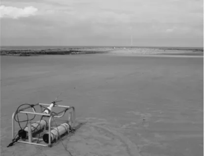
the ADV probe, with an accuracy of 1% of the measured value. Measure-ments have been performed in the beach in front of the research laboratory for Littoral and Coastal Ecosystems (ELICO): Eastern English Channel at Wimereux city (North of France, near Boulogne-sur-mer): this is a flat sand beach with a megatidal regime that varies between 8 to 11 m (see Figure 1). A heavy metallic structure has been built in the laboratory ELICO as a support for the ADV, its electronics canister, and its battery canister (see Figure 2). The measurement location is the intertidal zone in the beach, corresponding to the surf zone. The Eastern English Channel is a megatidal sea with strong currents. The metallic structure has been fixed to the ground using hooks; it was built in thin tubes to avoid a too strong stress on the structure from the tide and currents.

The measurements have been done on 9 and 10 June, 2004, during 2 tidal cy-cles, at a height of 50 cm from the bottom. Measurements have been considered when there was approximately at least 1 m of water above the experimental device. Due to the tidal activity, this distance was between 1 to 3 m. We con-sidered 27 sections of the U component of the velocity vector, corresponding to the direction perpendicular to the shore, each of length 32, 000 data points (each of 21 min duration). We cannot consider longer sections, since the in-ternal programming of the ADV interrupts the continuous recording of data, to synchronise the different clocks. The 27 sections have been chosen among the whole data set, in order to have a large enough internal correlation of

Fig. 2. A photography of the ADV measuring device and its support, in the intertidal zone, before being submerged by the tide.

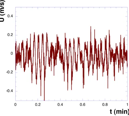
bursts, corresponding to a precise enough estimation of the velocity. We have thus a total of 864, 000 data points, separated into 27 sections. A one minute portion is shown in Figure 3: strong fluctuations at small scales are visible, but the whole time series seems stationary. In the following we analyze the data using the EMD method, the Hilbert-based amplitude-frequency method, and cumulant generating functions.

4.2 EMD applied to the data: amplitude-frequency pdf

We applied EMD analysis to surf zone velocity data using a EMD Matlab code kindly provided by Laboratoire de Physique (P. Flandrin, ENS Lyon, France): see the acknowledgements section for the web page. The analyses below are performed over the entire dataset, and the results displayed after performing an ensemble average over 27 realizations, where each segment of length 32, 000 data points is one realization. After decomposition, the original velocity series is decomposed into several IMFs (see Figure 4), from 13 to 16 modes (depending on the segment) with one residual. As visible in this figure, the time scale is increasing with the mode; each mode has a different mean frequency, which is estimated by considering the energy weighted mean frequency in the Fourier power spectrum of each mode time series; the relation between mode number m and mean time scale is displayed in Figure 5. The straight line which is obtained in log-linear plot suggests the following relation between the mean time scale T and m, for modes between 4 and 13:

Fig. 3. A one minute portion of the experimental velocity data, showing their high variability at small scales.

where T0 = 0.038 is a constant and the coefficient λ = 0.667 is graphically

estimated. We remark that eλ _{= 1.94 is close to 2, showing that each mode}

is associated with a time scale almost twice as large as the time scale of the preceding mode; this property corresponds to a dyadic filter bank in the time domain. This property was shown previously using stochastic simulations of Gaussian noise and fractional Gaussian noise (fGn) (Flandrin and Gon¸cal-v`es, 2004; Wu and Huang, 2004), and also for fully developed turbulence data (Huang et al., 2008). It is interesting to note here that this is still verified for surf zone turbulence data possessing a strong forcing in the middle of the studied range.

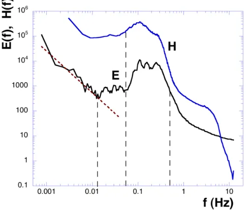
Figure 6 represents the averaged Fourier power spectrum of the data, super-posed with the Hilbert-Huang power spectrum. It is visible that the wind wave breaking scales (between 2 and 16 s) correspond to a strong forcing of the data. This power spectrum is similar to power spectra presented by Trowbridge and Elgar (2001) for surf zone turbulent data recorded in a sandy Atlantic beach near Duck, North Carolina. A −5/3 power spectrum can be found for large scales (minutes or larger) and scales smaller than 1 s could also be character-ized by such spectrum: the range is too small to be affirmative on this last point. The Hilbert-Huang spectrum which is superposed presents a similar shape, despite its different mathematical definition for the frequency as well as for the spectrum. For the smaller scales, the shape is different, since the

Fig. 4. IMFs estimated from one 32, 000 data points segment of the velocity time series: mode number increasing from top to below. The time scale is increasing with the mode. The residual time series is also plotted.

Fig. 5. Mean time scales associated with each mode. There is an exponential increase for mode numbers between 4 and 13.

Fig. 6. Fourier spectrum of the data (E(f )), superposed to the Hilbert marginal spectrum (H(f )). The latter has been vertically shifted for clarity. A strong wind wave breaking at scales between 2 and 16 s is clearly visible on both power spectra. It is interesting to notice that except for the smaller scales, they have the same shape, despite a different mathematical definition. The dotted straight line has a slope of −5/3.

Hilbert-Huang power spectrum falls down very quickly.

The EMD and Hilbert spectral analysis methodological frameworks provide a way to represent the fluctuations in an amplitude-frequency space: the joint pdf p(ω, A) is shown in Fig. 7. It can be seen graphically that the amplitudes decrease with increasing frequencies. This pdf can be used to estimate many statistical information such as the Hilbert spectrum, and the cumulants as shown below. It can also be used to estimate the skeleton As(ω) which

corre-sponds to the amplitude for which the conditional pdf p(A|ω) is maximum:

As(ω) = A0; p(A0, ω) = max_A {p(A|ω)} (14)

and the skeleton pdf pmax(ω) = p(As(ω), ω) = maxA{p(A|ω)}, which is shown

in Figure 8. A power law behaviour is found :

pmax(ω) ∼ ω−β2 (15)

cor-Fig. 7. Representation of the joint pdf p(ω, A) (in log scale) of velocity fluctuations in an amplitude-frequency space.

responds to an experimental fact that needs further investigation in future studies.

4.3 Non-analytic cumulant generating function: comparisons between struc-ture functions and EMD-Hilbert spectral approachs

We consider here the cumulant analysis applied to the velocity fluctuations, using the EMD and Hilbert spectral analysis described above, and compare this to the same analysis using structure functions.

We first show the estimation of the first cumulant c1 in Figure 9. In this

figure, the first cumulant is estimated as given by Eq.(10), using on the one hand, the amplitude-frequency pdf for a given value of ω, and taking the time scale ℓ = 1/ω (denoted “HSA” on the figure). On the other hand, it is superposed to the estimate of the first cumulants estimated for all modes separately, as function of scale, through the correspondence given by Figure 5 (denoted “EMD” in the figure). It is also superposed to the first cumulants estimated using the structure function approach, where the scale is the time increment: this value of c1 has been vertically shifted by 0.6 to be compared

to the other curves. Figure 9 shows that c1 increases strongly for energetic

scales associated with wave breaking, between 2 and 20 s. It also shows that the EMD-based first cumulant is very close to the Hilbert spectral analysis

−5 −4 −3 −2 −1 0 1 2 10−8 10−7 10−6 10−5 10−4 10−3 10−2 10−1 log10(ω) (Hz) pm a x ( ω ) 1.70

Fig. 8. The skeleton of the joint pdf pmax(ω) in log-log plot. A power law behaviour

is observed in the inertial subrange with scaling exponent 1.70.

0.01 0.1 1 10 100 1000 −0.6 −0.4 −0.2 0 0.2 0.4 0.6 !_(s) c1 HSA EMD SF (c1− 0.6)

Fig. 9. Estimation of the first cumulant c1, using three different methods: (i)

es-timation in frequency space using the joint amplitude-frequency pdf (dotted line denoted HSA); (ii) estimation using the empirical mode decomposition, done for each mode, where the time scale is estimated using the mode-scale correspondence (open dots, denoted EMD); and (iii) estimation using the structure functions.

0 1 2 3 4 5 6 7 8 0 1 2 3 4 5 6 q Φ ( !, q) Φ(!, q) ∼ 0.25q1.48 !_{= 2 (s) (q > 2)} (a) Ψ(!, q) − qC1(!) Fit 0.1 1 10 0.001 0.01 0.1 1 10 q Φ ( !, q) (b) Ψ(!, q) − qC1(!) Fit 0.1 1 10 0.001 0.01 0.1 1 10 q Φ ( !, q) (d) 0 1 2 3 4 5 6 7 8 0 1 2 3 4 5 6 7 q Φ ( !, q) _{Φ(!, q) ∼ 0.24q}1.55 !_{= 2 (s) (q > 2)} (c) Ψ(!, q) − qC1(!) Fit Ψ(!, q) − qC 1(!) Fit

Fig. 10. Φ(q) vs. q estimated for q between 0 and 8 for a scale ℓ = 2 s, chosen here for illustration purpose. Experimental values are given by continuous lines whereas dotted lines correspond to power-law fits. The proportionalities of Φℓ(q)

to qα confirm the nonanalytic framework applied here. (a): lin-lin plot using HSA mehod; (b): log-log plot using HSA method; (c) lin-lin plot using the structure functions; (d) log-log plot using the structure functions.

one (HSA). However the HSA approach is able to provide the first cumulant on a continuous range, since it is based on a frequency estimation, whereas the EMD curve is discrete in scale, being associated with the characteristic scale of each mode. We also see from this figure that the first cumulant estimated using the structure function is quite far from the other estimates: the plateau obtained at large scales comes from the fact that the differentce V (t+ℓ)−V (t) is not removing the forcing when the scale ℓ is larger than the forcing scale. This shows that for such data, the EMD and HSA methods provide a more reliable estimation of the first cumulant.

The functions Φ(q) are then estimated, for moments from 0 to 8, for scales between 1/25 s to 10 minutes. For comparison purposes, the analysis is done using the HSA approach in Equation (6) and using the structure functions. An example is shown in Figures 10a-d, for fluctuations at the scale of 2 s. Fig-ures 10a-b show the analyses using the HSA approach, in lin-lin and log-log plots, and Figures 10c-d show the same for the structure functions. Figures 10a and 10c show convex and increasing functions. The non-analytical behaviour

0.01 0.1 1 10 100 1000 1.3 1.35 1.4 1.45 1.5 1.55 1.6 1.65 1.7 1.75 1.8 !_(s) α ( !) αSF_{= 1.60 ± 0.07} αHSA_{= 1.52 ± 0.07} HSA SF

Fig. 11. Values of α estimated for different scales ℓ: comparison between the HSA and structure functions methods.

of these curves are emphasized in log-log plots (Figures 10b and 10d). The straight lines which are obtained confirm the non-analycity. Using a best fit, the slopes of these straight lines are estimated for all scales, giving directly the exponent α in Eq. (12). Figure 11 shows the values of α estimated for differ-ent scales ℓ, for both the HSA and the structure function methods. Except at both ends, the values are relatively independent of scale, and we can estimate a mean value: we find α = 1.52±0.07 for the HSA estimates and α = 1.60±0.07 for the structure functions estimates, where error bars are coming from differ-ent scales. These values are below 2 and approximately compatible between the two methods. Figure 12 shows the non-analytical cumulant (it cannot be denoted second cumulant) cα(ℓ) given by Equation (11). The curves are

dif-ferent for both methods, but their mean values are close. These results show that the log-normal framework is not adequate, to be replaced by a log-L´evy stochastic modelling. Simulations of such random variables can be performed using available stochastic simulation algorithms (Janicki and Weron, 1994).

5 Conclusion

We have considered here surf zone velocity measurements recorded in the East-ern English Channel using a 25 Hz sampling sonic anemometer. Such data is characterized by the transformation of wave motion into small-scale turbulent motion (Battjes, 1988). An important issue in this complex framework is to be able to characterize the contribution of each scale to velocity fluctuations, and hence to characterize velocity intermittency at many different time scales. The objective of this study was mainly to compare two different methods for

0.01 0.1 1 10 100 1000 0.05 0.1 0.15 0.2 0.25 0.3 0.35 0.4 !_(s) cα ( !) cHSAα = 0.23 ± 0.06 cSFα = 0.25 ± 0.02 HSA SF

Fig. 12. Values of cα(ℓ) estimated for different scales ℓ: comparison between the

HSA and structure functions methods.

the analysis of velocity fluctuations in such shallow water, wave dominated situations.

We have analysed the velocity time series here using the EMD methodology, associated with Hilbert spectral analysis. We have provided the mode versus time scale relationship, showing that for such data base, the dyadic mode de-composition which has been found in Gaussian noise is still valid. We have also provided the Fourier and Hilbert Huang marginal spectrum, showing the high energy associated with wave breaking scales, between 2 and 20 s. In another section, we have analyzed the fluctuations at each scale using cumulants. The cumulants could be estimated on a continuous range of scales using the joint amplitude-frequency pdf of velocity fluctuations that was estimated using the EMD-HSA framework. The non-analytical properties of cumulants was shown for each scale, for both methods. We showed, using the first cumulant, that the structure function approach saturates at large scales, whereas the HSA based method is more precise in its scale approach; this therefore shows the strength and usefulness of this new EMD-HSA method combined to cumulant analysis. It was shown here to be efficient for surf zone velocity analysis, but could be also applied to other time series.

Let us note that our approach has considered the time series globally, while the depth of the water varied between 1 and 3 meters. It may be that some statistical properties depend on the depth of the water, requesting a more precise analysis, considering separately different sections of the time series. We have checked that this is indeed the case (not shown here), considering the power spectra; however, the shape of the latter did not vary much. We then keep for future studies a more precise analysis of the depth relation,

noting here that the results we obtained must be considered as a mean value for different depths between 1 and 3 meters.

We have shown that the log-stable model applies very well, with a characteris-tic exponent of α = 1.60 ± 0.07 valid for all scales. This property may be used for stochastic simulations. Such modelling in the surf zone may be useful for several applications, such as plankton-turbulence coupling, energetics studies associated with bloom formation, to fertilization processes, or feeding rate of small fishes, or also sediment transport characterization and modelling, which are associated, either linearly or nonlineary, with velocity fluctuations (Cox et al., 1996; Svendsen, 2005; Torres-Freyermuth et al., 2007).

Acknowledgements

This work is sponsored in part by the National Natural Science Foundation of China (No.10472063, No.10672096) and the Innovation Foundation of Shang-hai University. Y.H. is financed in part by a Ph.D. grant from the French Ministry of Foreign Affairs. We thank Dominique Menu for the realisation of the metallic structure serving as support for the ADV. The EMD Matlab codes used in this paper are written by P. Flandrin from laboratoire de Physique, ENS Lyon (France): http://perso.ens-lyon.fr/patrick.flandrin/emd.html. This work benefited from financial support by the Contrat de Plan Etat R´egion 2000-2006, including funds from the French R´egion Nord-Pas-de-Calais, the French Ministry of Research and the European Fund of Regional Development (FEDER 2000-2006). Useful comments from the referees are acknowledged.

References

Anselmet, F., Antonia, R. A., Danaila, L., 2001. Turbulent flows and inter-mittency in laboratory experiments. Plan. Space Sci. 49 (12), 1177–1191. Anselmet, F., Gagne, Y., Hopfinger, E. J., Antonia, R. A., 1984. High-order

velocity structure functions in turbulent shear flows. J. Fluid Mech. 140, 63–89.

Arneodo, A., Baudet, C., Belin, F., Benzi, R., Castaing, B., Chabaud, B., Chavarria, R., Ciliberto, S., Camussi, R., Chilla, F., 1996. Structure func-tions in turbulence, in various flow configurafunc-tions, at Reynolds number be-tween 30 and 5000, using extended self-similarity. Europhys. Lett. 34 (6), 411–416.

Balocchi, R., Menicucci, D., Santarcangelo, E., Sebastiani, L., Gemignani, A., Ghelarducci, B., Varanini, M., 2004. Deriving the respiratory sinus

arrhyth-mia from the heartbeat time series using empirical mode decomposition. Chaos Soliton Fract. 20 (1), 171–177.

Battjes, J. A., 1988. Surf Zone Dynamics. Annu. Rev. Fluid Mech. 20 (1), 257–291.

Boratav, O. N., 1997. On recent intermittency models of turbulence. Phys. Fluids 9, 1206.

Chen, J., Xu, Y. L., Zhang, R. C., 2004. Modal parameter identification of Tsing Ma suspension bridge under Typhoon Victor: EMD-HT method. J. Wind Eng. Ind. Aerodyn. 92 (10), 805–827.

Chen, S., Cao, N., 1995. Inertial range scaling in turbulence. Phys. Rev. E 52 (6), 5757–5759.

Chevillard, L., Roux, S., L´evˆeque, E., Mordant, N., Pinton, J. F., Arn´eodo, A., 2005. Intermittency of Velocity Time Increments in Turbulence. Phys. Rev. Lett. 95 (6), 64501.

Cohen, L., 1995. Time-frequency analysis. Prentice Hall.

Coughlin, K. T., Tung, K. K., 2004. 11-Year solar cycle in the stratosphere extracted by the empirical mode decomposition method. Adv. Space Res. 34 (2), 323–329.

Cox, D., Kobayashi, N., Okayasu, A., 1996. Bottom shear stress in the surf zone. J. Geophys. Res. 101 (C6), 14337–14348.

Delour, J., Muzy, J., Arn´eodo, A., 2001. Intermittency of 1D velocity spa-tial profiles in turbulence: a magnitude cumulant analysis. Eur. Phys. J. B 23 (2), 243–248.

Denny, M. W., Shibata, M. F., 1989. Consequences of Surf-Zone Turbulence for Settlement and External Fertilization. The Am. Nat. 134 (6), 859–889. Du Preez, H. H., McLachlan, A., Marais, J. F. K., Cockcroft, A. C., 1990.

Bioenergetics of fishes in a high-energy surf-zone. Mar. Biol. 106 (1), 1–12. Eggers, H. C., Dziekan, T., Greiner, M., 2001. Translationally invariant cumu-lants in energy cascade models of turbulence. Phys. Lett. A 281, 249–255. Feller, W., 1971. An introduction to probability theory and its applications.

New York: Wiley.

Flandrin, P., Gon¸calv`es, P., 2004. Empirical Mode Decompositions as Data-Driven Wavelet-Like Expansions. Int. J. of Wavelets, Multires. and Info. Proc 2 (4), 477–496.

Frisch, U., 1995. Turbulence: the legacy of AN Kolmogorov. Cambridge Uni-versity Press.

Gardiner, C. W., 2004. Handbook of Stochastic Methods . Springer, Berlin, third edition.

Huang, N. E., Shen, Z., Long, S. R., Wu, M. C., Shih, H. H., Zheng, Q., Yen, N., Tung, C. C., Liu, H. H., 1998. The empirical mode decomposition and the Hilbert spectrum for nonlinear and non-stationary time series analysis. Proc. R. Soc. London 454 (1971), 903–995.

Huang, N. E., Shen, Z., Long, S. R., et al., 1999. A new view of nonlinear water waves: The Hilbert Spectrum . Annu. Rev. Fluid Mech. 31 (1), 417–457. Huang, Y. X., Schmitt, F. G., Lu, Z. M., Liu, Y. L., 2008. An

amplitude-frequency study of turbulent scaling intermittency using Empirical Mode Decomposition and Hilbert spectral analysis. EPL. submitted.

Hwang, P. A., Huang, N. E., Wang, D. W., 2003. A note on analyzing nonlinear and nonstationary ocean wave data. Appl. Ocean Res. 25 (4), 187–193. Jaffe, B., Rubin, D., 1996. Using nonlinear forecasting to learn the

magni-tude and phasing of time-varying sediment suspension in the surf zone. J. Geophys. Res. 101 (C6), 14283–14296.

Janicki, A., Weron, A., 1994. Simulation and chaotic behavior of alpha-stable stochastic processes. New York: Marcel Dekker.

J´anosi, I., M¨uller, R., 2005. Empirical mode decomposition and correlation properties of long daily ozone records. Phys. Rev. E 71 (5), 56126.

Kida, S., 1991. Log stable distribution and intermittency of turbulence. J. Phys. Soc. Japan 60 (1), 5–8.

Kolmogorov, A. N., 1941. The local stucture of turbulence in incompressible viscous fluid for very large Reynolds’ numbers. C R Acad Sci USSR. 30, 299–303.

Long, S. R., Huang, N. E., Tung, C. C., Wu, M. L., Lin, R. Q., Mollo-Christensen, E., Yuan, Y., 1995. The Hilbert techniques: an alternate ap-proach for non-steady time series analysis. IEEE Geoscience and Remote Sensing Soc. Lett. 3, 6–11.

Loutridis, S. J., 2004. Damage detection in gear systems using empirical mode decomposition. Eng. Struct. 26 (12), 1833–1841.

Loutridis, S. J., 2005. Resonance identification in loudspeaker driver units: A comparison of techniques. Appl. Acoust. 66 (12), 1399–1426.

Masselink, G., Russell, P., 2006. Flow velocities, sediment transport and mor-phological change in the swash zone of two contrasting beaches. Mar. Geol. 227 (3-4), 227–240.

Mead, K. S., Denny, M. W., 1995. The effects of hydrodynamic shear stress on fertilization and early development of the purple sea urchin

Strongylo-centrotus purpuratus. Biol. Bull 188 (1), 46–56.

Ponomarenko, V. I., Prokhorov, M. D., Bespyatov, A. B., Bodrov, M. B., Gridnev, V. I., 2005. Deriving main rhythms of the human cardiovascular system from the heartbeat time series and detecting their synchronization. Chaos Soliton Fract. 23, 1429–1438.

Pope, S. B., 2000. Turbulent Flows. Cambridge University Press.

Salisbury, J. I., Wimbush, M., 2002. Using modern time series analysis tech-niques to predict ENSO events from the SOI time series. Nonlinear Proc. Geoph. 9 (3/4), 341–345.

Schertzer, D., Lovejoy, S., 1987. Physical modeling and analysis of rain and clouds by anisotropic scaling multiplicative processes. J. Geophys. Res. 92 (D8), 9693–9714.

Schertzer, D., Lovejoy, S., Schmitt, F., Chigirinskaya, Y., Marsan, D., 1997. Multifractal cascade dynamics and turbulent intermittency. Fractals 5 (3), 427–471.

turbu-lence. Phys. Rev. Lett. 72 (3), 336–339.

Svendsen, I., 2005. Introduction to Nearshore Hydrodynamics. Adv. Series on Ocean Eng. 24.

Svendsen, I. A., 1987. Analysis of surf zone turbulence. J. Geophys. Res. 92 (C5), 5115–5124.

Taqqu, M. S., Samorodnisky, G., 1994. Stable Non-Gaussian Random Pro-cesses. Chapman & Hall, New York.

Torres-Freyermuth, A., Losada, I. J., Lara, J. L., 2007. Modeling of surf zone processes on a natural beach using reynolds-averaged navier-stokes equa-tions. J. Geophys. Res. 112, C09014.

Trowbridge, J., Elgar, S., 2001. Turbulence Measurements in the Surf Zone. J. Phys. Oceanogr. 31 (8), 2403–2417.

van de Water, W., Herwijer, J. A., 1999. High-order structure functions of turbulence. J. Fluid Mech. 387, 3–37.

Veltcheva, A. D., Soares, C. G., 2004. Identification of the components of wave spectra by the Hilbert Huang transform method. Appl. Ocean Res. 26 (1-2), 1–12.

Venugopal, V., Roux, S. G., Foufoula-Georgiou, E., Arn´eodo, A., 2006. Scaling behavior of high resolution temporal rainfall: New insights from a wavelet-based cumulant analysis. Phys. Lett. A 348 (3-6), 335–345.

Wu, Z., Huang, N. E., 2004. A study of the characteristics of white noise using the empirical mode decomposition method. Proc. R. Soc. London 460, 1597– 1611.