Relations between topography, wetlands, vegetation cover and stream water chemistry in boreal headwater catchments in Sweden

(1)

HAL Id: hal-00298950

https://hal.archives-ouvertes.fr/hal-00298950

Submitted on 29 May 2008

HAL is a multi-disciplinary open access

archive for the deposit and dissemination of sci-entific research documents, whether they are pub-lished or not. The documents may come from teaching and research institutions in France or abroad, or from public or private research centers.

L’archive ouverte pluridisciplinaire HAL, est destinée au dépôt et à la diffusion de documents scientifiques de niveau recherche, publiés ou non, émanant des établissements d’enseignement et de recherche français ou étrangers, des laboratoires publics ou privés.

Relations between topography, wetlands, vegetation

cover and stream water chemistry in boreal headwater

catchments in Sweden

J.-O. Andersson, L. Nyberg

To cite this version:

J.-O. Andersson, L. Nyberg. Relations between topography, wetlands, vegetation cover and stream water chemistry in boreal headwater catchments in Sweden. Hydrology and Earth System Sciences Discussions, European Geosciences Union, 2008, 5 (3), pp.1191-1226. �hal-00298950�

(2)

HESSD

5, 1191–1226, 2008 Relations between topography & stream

water chemistry J.-O. Andersson and

L. Nyberg Title Page Abstract Introduction Conclusions References Tables Figures ◭ ◮ ◭ ◮ Back Close

Full Screen / Esc

Printer-friendly Version Interactive Discussion Hydrol. Earth Syst. Sci. Discuss., 5, 1191–1226, 2008

www.hydrol-earth-syst-sci-discuss.net/5/1191/2008/ © Author(s) 2008. This work is distributed under the Creative Commons Attribution 3.0 License.

Hydrology and Earth System Sciences Discussions

Papers published in Hydrology and Earth System Sciences Discussions are under open-access review for the journal Hydrology and Earth System Sciences

Relations between topography, wetlands,

vegetation cover and stream water

chemistry in boreal headwater

catchments in Sweden

J.-O. Andersson1and L. Nyberg2

1

Department of Biology, Karlstad University, Universitetsgatan 2, 65188 Karlstad, Sweden

2

Department of Environmental Sciences, Karlstad University, Universitetsgatan 2, 65188 Karlstad, Sweden

Received: 2 April 2008 – Accepted: 11 April 2008 – Published: 29 May 2008 Correspondence to: J.-O. Andersson (jan-olov.andersson@kau.se)

(3)

HESSD

Full Screen / Esc

Printer-friendly Version Interactive Discussion

Abstract

A large part of the spatial variation of stream water chemistry is found in headwater streams and small catchments. To understand the dominant processes, taking place in small and heterogeneous catchments, spatial and temporal data with high resolu-tion is needed. In most cases available map data has too low quality and resoluresolu-tion 5

to successfully be used in environmental assessments and modelling. In this study 18 forested catchments (1–4 km2) were selected within a 120×50 km area in the county of V ¨armland in western Sweden. The aim was to test if topographic and vegetation variables derived from official datasets were correlated to stream water chemistry, rep-resented by DOC, Al, Fe and Si content. A GIS was used to analyse the elevation 10

characteristics, generate topographic indices and calculate the percentage of wetlands and a number of vegetation classes. The results clearly show that the topography has a major influence on the occurrence of wetlands, which has a major influence on stream water chemistry. There were very strong correlations between mean slope and percentage wetland, percentage wetland and DOC, mean slope and DOC and mean 15

topographic wetness index and DOC. The conclusion was that official topographic data, despite uncertain or low quality and resolution, could be useful in the prediction of headwater chemistry in boreal forested catchments.

1 Introduction

The chemistry of headwater streams is influenced by several landscape factors, which 20

are related to geology, topography, climate and vegetation. During the 20th century, the human impact has also been significant, even for the smallest water systems, for example internal impact from land use measures and external impact from atmospheric deposition.

In Nordic boreal forests, some landscape factors are especially important for the de-25

(4)

HESSD

Full Screen / Esc

Printer-friendly Version Interactive Discussion (granite and gneiss), which results in acid-sensitive waters with a low content of

dis-solved substances. Another typical factor is the multitude of wetlands, which give a typical influence of dissolved organic matter, and consequently an increased natural acidity. This condition was for example clearly showed in data used by Andersson and Nyberg (2008), where about 60% of 68 randomly selected boreal headwater streams 5

had a water colour (at medium flow) above 100 mg Pt/l, which corresponds to the high-est class of five in the Environmental Quality Criteria, high-established by the Swedish En-vironmental Protection Agency (SNV, 2003).

Because of the severe acidification problems that have been a dominant environmen-tal condition in forested areas in for example Sweden and Norway for several decades, 10

and the ambition to separate the anthropogenic and natural acidity (SEPA, 2003), there is an interest in understanding how landscape factors influence stream water chemistry and especially those factors that govern the acidity.

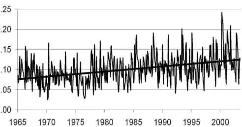
The forested landscape in Sweden also experiences a long-term increase in dis-solved organic matter. This could be exemplified by the trend for absorbance in River 15

Klar älven (Fig. 1), which is a larger river situated near the area studied in this paper. The increase has been +50% over 40 years. The reason for the increase in this par-ticular case is not fully investigated, but in the literature, climate changes (Clair et al., 1994; Freeman et al., 1995; Moore, 1998; Tranvik et al., 2002; Worall et al., 2003; L öfgren et al., 2003) and intensified forestry (Ros én et al., 1996; Lundin, 1999) are 20

suggested as factors behind long-term changes in dissolved organic matter. A third potential factor can be decreased deposition of sulphur (Monteith et al., 2007).

There seems to be a gap between hydrological process-oriented research and the institutions that are dependent on methods and results in their work of solving regional and national environmental problems. The process knowledge is mostly available from 25

studies of soil profiles, hillslopes or smaller catchments, and the need for tools is most obvious at a larger scale. One reason for the dominance of small-scale studies is the large spatial and temporal variability of factors that determine the hydrology and hydrochemistry. E.g. Wolock et al. (1997) showed that stream chemistry variability

(5)

sig-HESSD

Full Screen / Esc

Printer-friendly Version Interactive Discussion nificantly decreased beyond catchment sizes of 3–4 km2. Another reason concerns the

possibilities to measure. Hooper (2001), e.g. concludes that “the instruments measure at a scale of decimetres when we need to understand the landscape at the scale of hectares or square kilometres”. A third reason might be that forest hydrology research has been closely linked to acidification research for several decades, and most of the 5

acidification problems are found at higher altitudes near the headwaters.

There is a need for simpler, less time consuming and less costly methods to predict head water chemistry in the evaluation of the natural state of water quality, in order to make correct decisions for protection and restoration measures (SNV, 2003).

To reduce the gap between small-scale process knowledge and demands for better 10

understanding at larger scales, one can study smaller elements that are aggregated into larger systems (Sivapalan and Kalma, 1995; Bl ¨oschl and Sivapalan, 1995). In doing this up-scaling, it is necessary to integrate new tools and data, such as late de-velopments of GIS and official regional or national databases, into the analysis. For hydrology and hydrochemistry, the process knowledge gained from hillslope studies 15

and small experimental catchments, needs first to be evaluated at the next larger scale, i.e. larger first-order and second-order streams. Bl ¨oschl (1995) suggested that instead of trying to capture everything when upscaling it would be better to identify dominant processes that control hydrological response at different scales, and then develop mod-els to focus on these dominant processes. When going into larger scales, in-stream 20

and hyporheic processes will be more important, and a crucial scale-step is when the streams flow into the first lake, which, depending on size, could have a large impact on hydrology and hydrochemistry.

1.1 Topography

Research results from the latest decades clearly show an influence of topography and 25

wetland on stream water chemistry. The influence of topography is important since it controls the water subsurface contact time (Beven and Kirkby, 1979; Wolock et al.,

(6)

HESSD

Full Screen / Esc

Printer-friendly Version Interactive Discussion 1990; Dillon and Molot, 1997). Since the beginning of 1990’s many methods for

de-riving these attributes from elevation data have been developed for use in hydrological applications. These attributes can be divided in two groups: primary and secondary topographic attributes.

Slope is a primary attribute that measures the rate of change of elevation and the 5

direction of steepest decent, and the means by which gravity induces flow of water. Thus, it is of great significance in hydrology, affecting soil water content, flowpaths and residence times (Nyberg, 1995), and subsequently the chemical composition of surface waters (Beven, 1989; Wolock et al., 1989). Mean slope, based on a DEM with 50 m grid, was a variable that correlated with headwater chemistry in a previous study in the 10

same region as in this paper (Andersson and Nyberg, 2008). Slope can be derived from elevation data by calculations in GIS or other computer softwares.

A secondary attribute, the topographic wetness index ln(a/tan β), where a is the upslope area per unit contour length and tan β is the slope, (Beven and Kirkby, 1979; Quinn et al., 1995), has frequently been used in modelling, and represents the wetness 15

distribution in a catchment. A high value of the index means that the groundwater table is likely to be close to the ground surface. Subsequently, wetlands occur in areas with high values of the topographic wetness index, and it would be possible to predict loca-tions of these by calculating topographic wetness indices over catchments. However, the possibility of doing this successfully depends on the relation between the spatial 20

resolution of the data used in the index calculation and the typical length scales of the topography in the catchment (Rodhe and Seibert, 1999). The scale and terrain rough-ness of the analysed landscape and the resolution of the elevation data sets limits for the quality of the result (Moore et al., 1993; Wolock et al., 1994). Topographic indices can give valuable information about the distribution of soil moisture, location of poten-25

tial saturated zones and source areas for runoff generation. The calculation of wetness indices is, however, sensitive to the used algorithm (G ¨untner et al., 2004). Especially the calculation of the upslope contributing area is crucial for the resulting pattern of saturated areas.

(7)

HESSD

Full Screen / Esc

Printer-friendly Version Interactive Discussion 1.2 Wetlands, vegetation cover and dissolved organic matter

In the Swedish boreal landscape, mire, divided into bogs, fens and mixed mires, is the most common wetland group (L ¨ofroth, 1991). The occurrence of wetlands in bo-real headwater catchments has in several studies shown a significant correlation with stream chemistry. Processes in peat and other frequently saturated organic soils pro-5

duce humic substances that are transported to streams (Clair et al., 1994; Dillon and Molot, 1997; Mulholland and Kuenzler, 1979; Eckhardt et al., 1990; Koprivnjak and Moore, 1992; Hope et al., 1994; Mulholland, 1997). Hemond (1990) suggested that the most important processes take place in the riparian zone and depends on the stream flow generation. He was supported by Bishop et al. (1994) but questioned by K ¨ohler et 10

al. (1999) who concluded that the question of how organic acids enter streams still was open. Andersson and Nyberg (2008) concluded from a study of 68 headwater streams that it did not seem possible to predict humic substances in headwater streams by sim-ply looking at the occurrence and locations of wetlands that are shown on official maps. Many small or hidden wetlands, or “cryptic wetlands” (Creed et al., 2003), with shal-15

low peat cover are not shown on official maps because they are difficult or impossible to locate on aerial photos. Still, they are possible sources of production of dissolved organic matter in headwater catchments.

1.3 Objectives

The main objective of this study was to analyse the relations between topography, 20

wetland and vegetation cover, represented by available official landscape data, and chemistry in boreal headwater streams in western Sweden. The aim was to determine “dominant landscape variables” that control the transport of dissolved organic matter, which is closely associated with natural acidification. However, data on soils (type, texture) and bedrock (type) was not included in the study as spatial datasets, since the 25

available official maps have too low accuracy and spatial resolution. Furthermore, data on vegetation cover generally reflects the distribution of soil types well (Moore et al.,

(8)

HESSD

Full Screen / Esc

Printer-friendly Version Interactive Discussion 1991).

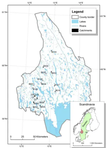
2 Study area

The 18 studied catchments were located within a 120×50 km area in the county of V ¨armland in western Sweden, between latitude 59 and 61 degrees N and longitude 12 and 14 degrees E (Fig. 2).

5

The dominant landform in the area is a hilly relief with some occurrence of faults and bare bedrocks in the south and higher but gentler hills in the north. The igneous bedrock consists mainly of acidic granites and gneisses with some occurrence of out-crops of magmatic hyperite and other rock types (Lundeg ˚ardh, 1995). The dominant soil type is till (>65%), peat (∼20%) and some areas with sand and silt. The area 10

contains lakes and wetlands while only a small part (<10%) is covered by farmland. The average elevation is approx. 200 m a.s.l. and the highest marine shoreline lies be-tween 170 and 210 m a.s.l. within the area (Lundqvist, 1958, 1961). The annual mean temperature is 3–5◦_{C, precipitation 800–900 mm, runoff 400–450 mm and}

evapotran-spiration 400–450 mm. The precipitation normally falls as snow between November 15

and mid March. The peak runoff normally occurs during the snowmelt period (Raab and Vedin, 1995). Coniferous forests (Picea abies and Pinus sylvestris) dominate the area. Within the area, only forestry can be counted as human impact of larger extent. However, the area has suffered from deposition of sulphur and nitrogen (Lundstr ¨om et al., 1998).

20

3 Methods

1:250 000 and 1:100 000 scale official topographic maps from the Swedish Land Survey were used to delimit an area within the western part of the county of V ¨armland. 18 first-order streams were selected within the area for this study. The streams were

(9)

HESSD

Full Screen / Esc

Printer-friendly Version Interactive Discussion part of two previous studies: 14 streams were taken from a study of 76 first-order

streams, described by Andersson and Nyberg (2008). The other four were taken from a hydrological restoration project called “The Laskerud Project”. The streams were first or second order. No arable or urban land was included in the 18 catchments. Forestry occurs in the catchments but was estimated not to be of the magnitude of influence to 5

be considered in this study. 3.1 Spatial datasets

1:50 000 and 1:20 000 scale official topographic maps from the Swedish Land Survey were scanned and used for delineation of the catchments. Streams, wetlands and contour lines were digitized. The contours were used for delineation of catchments. 10

The topographic maps were rather coarse in relation to the size of the catchments in this study. The maps show larger wetlands (>0.5 ha) and the generalization is rather strong. During field surveys some of the contour delineated water divides were found incorrect. Depending on the thickness of the vegetation and the roughness of the terrain the accuracy of the contour lines varied significantly.

15

An official 50 m resolution digital elevation model (DEM) and vegetation data were obtained from the Swedish Land Survey. The DEM has a mean elevation error of 2.5 m. The vegetation data was produced by interpretation of infrared aerial photos and has comparatively high spatial accuracy.

3.2 GIS analysis 20

ArcInfo GIS was used for calculations of area, elevation, slope and Topographic Wet-ness Index (TWI) layers for each catchment. TWI=ln(a/tan β), where a is the upslope area per unit contour length and tan β is the slope gradient. The calculation of the upslope area was based on a deterministic 8 model (O’Callagan and Mark, 1984) for flow over a terrain surface represented by the DEM. The mean value of the slope and 25

(10)

HESSD

Full Screen / Esc

Printer-friendly Version Interactive Discussion The percentage of each vegetation type within the catchments was calculated. The

digitized wetlands from the 1:50 000 scale maps were managed in the same way and compared with the mire types extracted from the vegetation data. The mires were classed into fen, bog and mixed mires.

3.3 Water sampling and chemical analysis 5

Water samples were collected at the outlet of each catchment four times at different flow situations during different seasons: summer low flow, summer medium flow (#1), autumn medium flow (#2) and spring high flow. 14 of the streams were sampled in 1998 and 1999 during four campaigns. The chemistry data from the four streams in the Laskerud Project were selected from a time series from 2003 and 2004. The selection 10

was based on season and specific discharge. The filtered samples were kept dark and cool until the concentration of DOC [mg/l] was determined. The instrument used for measuring the DOC-concentration was a Schimadzu 500 carbon-analyser. Fe, Al and Si were analysed with ICP-OES (Varian).

The runoff was estimated by simple methods (bucket or float) when the samples 15

were taken. The specific runoff was in average 0.8 l/s/km2 at the low flow situation, 13 l/s/km2 at the medium flow #1 situation, 11 l/s/km2at the medium flow #2 situation and 30 l/s/km2 at the high flow situation. During the high flow sampling round, seven streams were not sampled due to snow covered roads that made the sites inaccessible. 3.4 Statistical analysis

20

PCA analysis was initially performed to study the overall relations between topographic, wetland and vegetation variables. Correlation (Pearson) and linear regression analy-ses were then performed in order to investigate the covariation between landscape variables and water chemistry at different flow situations.

(11)

HESSD

Full Screen / Esc

4 Results

4.1 Topographic characteristics

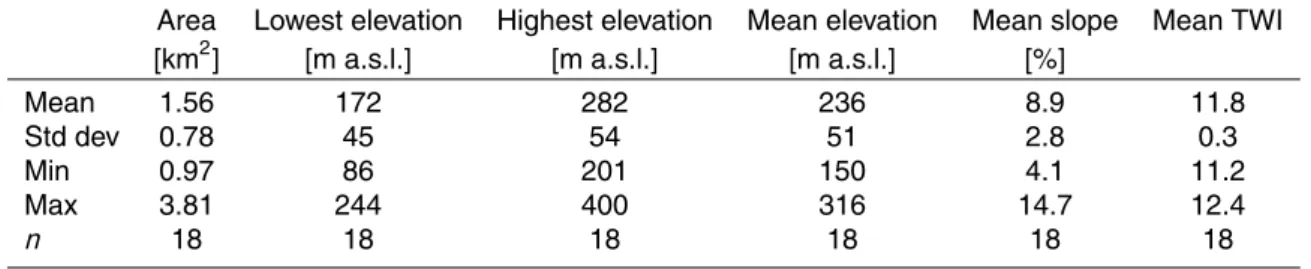
The mean size of the 18 catchments was 1.56 km2(Table 1). Most of the catchments were situated above the highest marine shoreline, which is at about 180–190 m a.s.l. Catchment L5 has been selected to visualize the spatially distributed data used in the 5

analysis (Fig. 3a–c). L5 was the catchment with highest percentage of wetland, 20%. It was also the catchment with lowest mean slope, 4.1%. The topographic wetness index for single 50×50 m cells ranged from 9.6 to 19.1 with a mean of 12.4.

Mean slope and mean topographic wetness index were strongly negatively corre-lated to each other, which was expected since the calculation of TWI includes the slope 10

in the denominator. The correlation coefficient of −0.95 indicated that the slope has a dominant influence in the TWI, compared to the upstream drainage area per contour length a.

4.2 Wetland characteristics

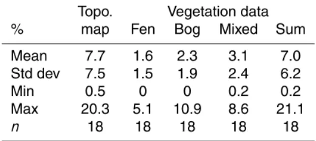
In average 7% of the area of the 18 studied catchments were covered with wetland 15

(Table 2). The wetland percentage on the 1:50 000 scale maps was 0.7% larger than the percentage in the vegetation data. About 40% of the wetland was mixed mire according to the vegetation data.

There were only small differences in the distribution and location of wetlands in the two types of data sources. The errors are mainly caused by misinterpretations between 20

wet coniferous forest and coniferous mire. There is no distinction between mire classes in the topographic map. Figure 4 exemplifies the distribution of fen, bog and mixed mire in Catchment L5. Bogs covered 11%, mixed mires covered 5.1% and fens covered 5.1% of the catchment. Figure 5 shows the same catchments’ mire types represented in the vegetation database.

(12)

HESSD

Full Screen / Esc

Printer-friendly Version Interactive Discussion 4.3 Vegetation characteristics

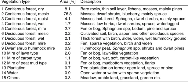
The vegetation database included 22 vegetation types within the catchments, of which the 7 smallest were merged and categorized as “others”. The catchments were domi-nated by mesic coniferous forest (77%). Dry coniferous forest covered 8.1% and moist coniferous forest 4.1%. Of the mire vegetation types the lawn type (2.0%) and carpet 5

type (1.1%) was most common (Table 3). In Table 4 the occurrence of the different vegetation types in each catchment is listed.

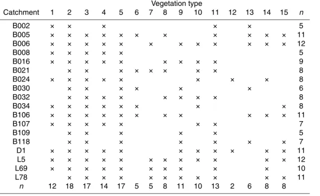
There is a large heterogeneity regarding vegetation types within and between the catchments (Table 4). Catchment B008 and B109 only comprise five vegetation types while catchment B006 and L5 had twelve. The table also shows the frequency of 10

the vegetation types. Mesic coniferous forest was found in every catchment. Moist coniferous forest was found in all but one, while others were less frequent.

4.4 Chemical characteristics

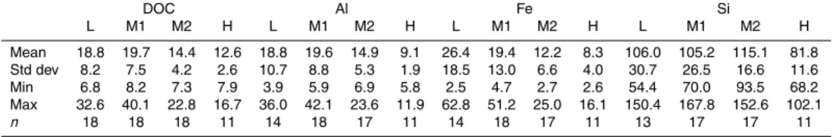
DOC was used as a measure of dissolved organic matter. The DOC levels in the studied catchments were relatively high (Table 5), and the temporal and spatial varia-15

tions were large (Fig. 7). The highest levels were found for the low and medium flow samplings. The low and summer medium flow samplings had lower levels of DOC. Si, which is a measure of silicate weathering, had highest concentrations during the autumn medium flow and lowest during the spring flood.

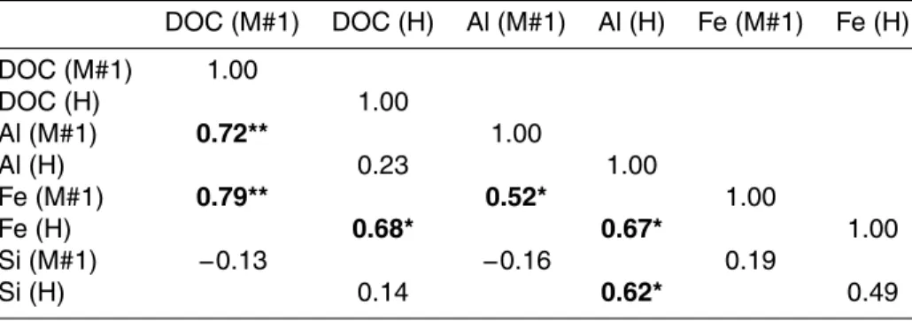
Fe (Fig. 6), Al and Si were correlated to DOC (Table 6), and had similar seasonal 20

patterns as DOC.

The greatest temporal variability was found in catchment B021 where the DOC level ranged from 0.11 at high flow to 0.35 at medium flow 2. In B021 the mean DOC level was 0.19 while it was as low as 0.02 in catchment B002.

(13)

HESSD

Full Screen / Esc

Printer-friendly Version Interactive Discussion 4.5 Relations between topography, wetland and vegetation

A principal component analysis (PCA) including all topographic and vegetation ables was carried out to investigate the relations between those two groups of vari-ables (Fig. 8). The first principal component explained 40% of the total variation, and captured primarily the slope-related variation. The second component explained 22%, 5

and described the variation related to elevation.

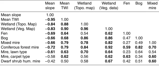
There was a group of variables that contributed most to PC1: mean slope, mean TWI, total wetland and coniferous forest of mire type. These four variables were also strongly correlated to each other. A further analysis of the relation between coniferous mire type and total wetland showed that a rather stable proportion of 40% of the total 10

wetland in each catchment was of coniferous mire type.

In PC2, dry coniferous forest had the strongest (negative) correlation with altitude. This is probably a side-effect of the weak correlation between altitude and latitude. The mean altitude was slightly higher in the northern part of the study area, where the soil cover is somewhat deeper.

15

A correlation analysis for topographic and wetland variables was made (Table 7). The strongest correlation was found between mean topographic wetness index and wetland percentage estimated from the vegetation map (Fig. 9).

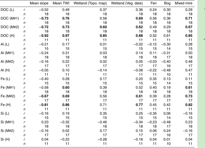
4.6 Relations between topography-wetland-mires classes and water chemistry A correlation analysis including topography, wetland percentages and water chemistry 20

(Table 8) showed moderate and strong pair-wise correlations between topography-wetland, wetland-chemistry and topography-chemistry. The chemistry referred to here is DOC and Fe during medium and high flow. The correlations between topogra-phy/wetland and DOC/Fe were especially high during high flow.

The classification of wetlands into bogs and fens did not give any stronger corre-25

lations in relation to water chemistry (Table 8). The class “Mixed mire” had stronger correlations than “Fen” and “Bog”.

(14)

HESSD

Full Screen / Esc

Printer-friendly Version Interactive Discussion Si was not significantly correlated to topography or wetland.

There was a strong correlation between mean topographic wetness index and DOC (Table 8, Fig. 10). It was strongest at the high flow situation and decreasing with decreasing flow.

5 Discussion

5

The results show several strong correlations between topography, wetlands and DOC. The vegetation data, however, did not bring much to the results, even if there were some significant correlations. The vegetation database was, however, useful for vali-dation of the topographic map data.

The topography and wetland variables were stronger correlated to the water chem-10

istry at medium (summer and autumn) and high flow (spring flood) than at the low flow situation (summer). This indicated that, for this 120×50 km area, the connection be-tween the sources of dissolved organic carbon and the stream was weaker during low flow. One possible reason was the longer retention times for water in the ground and streams which gave more time for biological degradation of organic matter. The low 15

flow situation also occurred during summer when the biological activity was high. A previous study in the same region concluded that the variable “mean slope” was better correlated to DOC than the occurrence of wetlands in headwater catchments (Andersson and Nyberg, 2008). That study also concluded that better quality and higher resolution of spatial data are needed in order to make reliable estimates of 20

influencing factors in head water catchments smaller than 1.5 km2.

It is widely recognized that topographic analyses are sensitive to the resolution of the data source generalized. This affects all topographic attributes, but in varying ways. The resolution-dependence of slope and specific catchment area has been most in-tensively studied because of their regular application in hydrological modelling (e.g. 25

Tarboton, 1997; Moore et al., 1993; Zhang and Montgomery, 1994). In this study a 50 m DEM grid was used for deriving the variables “slope” and “topographic wetness

(15)

HESSD

Full Screen / Esc

Printer-friendly Version Interactive Discussion index”, which were used in statistical analyses of the complex interactions taking place

in small scale heterogeneous boreal catchments.

Beven (1997) criticized modellers deriving topographic indices from DEMs with grid sizes exceeding slope lengths in the landscape. Comparing the topographic wetness index grid with the wetland layer in this study was not a success. This was also tested 5

by Rodhe and Seibert (1999) with varying results. Our study supports their conclusion that the geologic conditions modify the topographic control of the wetness. S ¨orensen and Seibert (2007) concluded that the DEMs with different grid resolution showed con-siderable differences in the TWI pattern. That statement will be a question for further studies in our study area when better elevation data is obtained.

10

The final conclusion is, however, that very strong correlations between DOC and mean topographic wetness index and wetland percentage (especially at high flow sit-uations) indicate that available spatial data (official 1:50 000 scale topographic maps and 50 m DEM grids) could be used for predictions of stream water chemistry (DOC and iron) in headwater catchments in Swedish boreal forests.

15

Acknowledgements. The authors wish to thank Mistra (The Foundation for Strategic

Environ-mental Research) and the multi-disciplinary research group Milj ¨oFoCus at Karlstad University for funding. Maria Malmstr ¨om is gratefully thanked for her work with chemical analyses.

References

Andersson, J. O. and Nyberg, L.: Spatial variation of wetlands and flux of dissolved organic

20

carbon in boreal headwater streams, Hydrol. Processes, 22, 1965–1975, 2008.

Beven, K. J. and Kirkby, M. J.: A physically based, variable contributing area model of basin hydrology, Hydrol. Sci. B., 24, 43–69, 1979.

Beven, K. J.: Hillslope runoff processes and flood frequency characteristics, in: Hillslope Pro-cesses, edited by: Abrahams A. D., 187–202, Allen and Unwin, Boston, 1986.

25

Beven, K. J.: Topmodel: a critique, Hydrol. Processes, 11, 1069–1085, 1997.

Bishop, K. H., Petterson, C., Allard, B., and Lee, Y. H.: Identification of the riparian sources of aquatic dissolved organic carbon, Environ. Int., 20(1), 11–19, 1994.

(16)

HESSD

Full Screen / Esc

Bl ¨oschl, G.: Scaling in hydrology, Hydrol. Processes, 15, 709–711, 2001.

Bl ¨oschl, G. and Sivapalan, M.: Scale issues in hydrological modelling: A review, Hydrol. Pro-cesses, 9(3–4), 251–290, 1995.

Clair, T. A., Pollock, T. L., and Ehrman, J. M.: Exports of carbon and nitrogen from river basins in Canada’s Atlantic provinces, Global Biogeochem. Cycles, 8, 441–450, 1994.

5

Creed, I. F., Sanford, S. E., Beall., F. D., Molot, L. A., and Dillon, P. J.: Cryptic wetlands: integrating hidden wetlands in regression m0odels of the export of dissolved organic carbon from forest landscapes, Hydrol. Processes, 17, 3629–3648, 2003.

Dillon, P. J. and Molot, L. A.: Effect of landscape form on export of dissolved organic carbon, iron, and phosphorus from forested stream catchments, Water Resour. Res., 33, 2591–2600,

10

1997.

Eckhardt, B. W. and Moore, T. R.: Controls on dissolved organic carbon concentrations in streams, southern Quebec, Can. J. Fish. Aquatic Sci., 47, 1537–1544, 1990.

Freeman, C., Gresswell, R., Lock, M. A., Swanson, C., Guasch, H., Sabater, F., Sabater, S., Hudson, J., Hughes, S., and Reynolds, B.: Climate change: Mans indirect impact on wetland

15

microbial activity and the biofilms of a wetland stream, in: Man’s Influence on Freshwater Ecosystems and Water Use, International Association of Hydrological Sciences Publication, 230, 199–206, 1995.

Grayson, R. B. and Bl ¨oschl, G.: Spatial Patterns in Catchment Hydrology: Observations and Modeling, Cambridge University Press, 2000.

20

G ¨untner, A., Seibert, J., and Uhlenbrook S.: Modelling spatial patterns of saturated areas: An evaluation of different terrain indices, Water Resour. Res., 40, W05114, doi:10.1029/2003WR002864, 2004.

Hemond, H. F.: Wetlands as the source of dissolved organic carbon to surface waters, Organic Acids in Aquatic Ecosystems, 301–131, 1990.

25

Hooper, R. P.: Applying the scientific method to small catchment studies: a review of the Panola Mountain experience, Hydrol. Processes, 15, 2039–2050, 2001.

Hope, D., Billett, M. F., and Cresser, M. S.: A review of the export of carbon in river water: fluxes and processes, Environ. Pollut., 84, 301–324, 1994.

K ¨ohler, S., Hruska, J., and Bishop, K.: Influence of organic acid site density in pH modeling of

30

Swedish lakes. Can. J. Fish. Aquatic Sci., 56(8), 1461–1470, 1999.

Koprivnjak, J.-F. and Moore, T. R.: Sources, sinks, and fluxes of dissolved organic carbon in subarctic fen catchments, Arctic and Alpine Res., 24, 204–210, 1992.

(17)

HESSD

Full Screen / Esc

Lundeg ˚ardh, P. H.: Beskrivning till berggrundskartan över V ärmlands l än: östra och meller-sta V ärmlands berggrund: fyndigheter av nyttosten och malm i V ärmlands l än, Serie Ba,

¨

Oversiktskartor med beskrivningar, 45:1/03732657, Sveriges Geologiska Unders ¨okning, Stockholm, Sweden, 1995 (in Swedish).

Lundin, L.: Effects on hydrology and surface water chemistry of regeneration cuttings in

peat-5

land forests, Int. Peat J., 9, 118–126, 1999.

Lundqvist, J.: Studies of the quaternary history and deposits of V ¨armland, Sweden. Swedish Geological Survey, Yearbook 1958, 52(2), Stockholm, Sweden.

Lundqvist, J.: Beskrivning till karta över landisens avsm ältning och h ögsta kustlinjen i Sverige, Sveriges Geologiska Unders ökning, Stockholm, Sweden, ser Ba nr 18, 1961 (in Swedish).

10

Lundstr ¨om, U., Nyberg, L., Danielsson, R., van Hees, P., and Andersson, M.: Forest soil acid-ification: Monitoring on the regional scale exemplified in V ¨armland, Sweden, Ambio, 27(7), 551–556, 1998.

L ¨ofgren, S., Andersen, T., and Forsius, M.: Climate induced water color increase in Nordic lakes and streams due to humus, Nordic Council of Ministry brochure, 2003.

15

L ¨ofroth, M.: V ˚atmarkerna och deras betydelse, Rapport 3824, Naturv ˚ardsverket, Solna, Swe-den, 1991 (in Swedish).

McGuire, K. J., Mc Donnel, J. J., Weiler, M., McGlynn, B. L., Welker, J. M., and Seibert, J.: The role of topography on catchment-scale water residence time, Water Resour. Res., 41, W05002, doi:10.1029/2004WR003657, 2005.

20

Monteith, D. T., Stoddard, J. L., Evans, C. D., de Wit, H. A., Forsius, M., Høgasen, T., Wilander, A., Skjelkvale, B. L., Jeffries, D. S., Vuorenmaa, J., Keller, B., Kopacek, J., and Vesely, J.: Dissolved organic carbon trends resulting from changes in atmospheric deposition chemistry, Nature, 450, 537–540, 2007.

Moore, I. D., Grayson, R. B., and Landson, A. R.: Digital Terrain Modelling: a Review of

Hydro-25

logical, Geomorphological, and Biological Applications, Hydrol. Processes, 5, 3–30, 1991. Moore, I. D., Lewis, A., and Gallant, J. C.: Terrain attributes: Estimation methods and scale

effects, Modelling Change in Environmental Systems, edited by: Jakeman, A. J., Beck, M. B., and McAleer, M., John Wiley and Sons Ltd, chapter 8, 1993.

Moore, I. D., Gallant, J. C., Guerra, L., and Kalma, J. D.: Modelling the spatial variability of

30

hydrological processes using Geographical Information Systems, edited by: Kovar, K. and Nachtnebel, H. P., HydroGIS 93: Application of Geographical Information Systems in Hydrol-ogy and Water Resources, IAHS Pubn., 211, 161–169, 1993.

(18)

HESSD

Full Screen / Esc

Moore, T. R.: Dissolved organic carbon: sources, sinks, and fluxes and role in the soil carbon cycle, in: Soil Processes and the Carbon Cycl., edited by: Lal, R., Kimble, J. M., Follett, R. F., and Stewart, B. A., Adv. Soil Sci., CRC press, Boca Raton, FL., 281–292, 1998.

Mulholland, P. J. and Kuenzler, E. J.: Organic carbon export from upland and forested wetland watersheds, Limnol. Oceanogr., 24, 960–966, 1979.

5

Mulholland, P. J.: Dissolved organic matter concentration and flux in streams, J. North Am. Benthological Soc., 16, 131–141, 1997.

Nyberg, L.: Soil- and groundwater distribution, flowpaths and transit times in a small till catch-ment, PhD Thesis, Uppsala University, 1995.

O’Callaghan, J. F. and Mark, D. M.: The extraction of drainage networks from digital elevation

10

data, Comput. Vis. Graph. Image Process., 28, 323–344, 1984.

Quinn, P. F., Beven, K. J., and Lamb, R.: The ln(a/tan β) index: how to calculate it and how to use it in the TOPMODEL framework, Hydrol. Processes, 9, 161–182, 1995.

Rodhe, A. and Seibert, J.: Wetland occurrence in relation to topography – a test of topographic indices as moisture indicators, Agric. For. Meteorol., 98–99, 325–340, 1999.

15

Raab, B. and Vedin, H.: Klimat, sj ¨oar och vattendrag. Sveriges Nationalatlas, SNA f ¨orlag, Stockholm, Sweden, 1995 (in Swedish).

Ros ´en, K., Aronson, J. A., and Eriksson, H. M.: Effects of clear-cutting on stream water quality in forest catchments in central Sweden, For. Ecol. Manage., 83(3), 237–244, 1996.

SEPA: Natural acidification only, Report 5317, Swedish Environmental Protection Agency,

20

Stockholm, Sweden, 2003 (in Swedish with English summary).

SNV: Milj ökvalitetsnormer f ör fl öden/niv ˚aer i rinnande vatten, Redovisning av ett regeringsup-pdrag, Rapport 5292, Naturv ˚ardsverket, 2003 (in Swedish).

Sivapalan, M. and Kalma, J. D.: Scale problems in hydrology: Contributions of the Robertson workshop, Hydrol. Processes, 9(3–4), 243–250, 1995.

25

S ¨orensen, R. and Seibert, J.: Effects on the calculation of topographical indices: TWI and its components, J. Hydrol., 327, 79–89, 2007.

Tarboton, D. G.: A new method for the determination of flow directions and upslope areas in grid digital elevation models, Water Resour. Res., 33, 309–320, 1997.

Tranvik, L. J., Jansson, M., Evans, C. D., Freeman, C., Monteith, D. T., Reynolds, B., and

30

Fenner, N.: Climate Change: terrestrial export of organic carbon, Nature, 415, 861–862, 2002.

(19)

HESSD

Full Screen / Esc

catchment topography and soil hydraulic characteristics to lake alkalinity in the north eastern United States, Water Resour. Res., 25, 829–837, 1989.

Wolock, D. M., Hornberger, G. M., and Musgrove, T. J.: Topographic effects on flow path and surface water chemistry of the Llyn Brianne catchments in Wales, J. Hydrol., 115, 243–259, 1990.

5

Wolock, D. M. and Price, C. V.: Effects of digital elevation model map scale and data resolution on a topography-based watershed model, Water Resour. Res., 30(11), 3041–3052, 1994. Wolock, D. M., Fan, J., and Lawrence, G. B.: Effects of basin size on low-flow stream chemistry

and subsurface contact time in the Neversink river watershed, New York, Hydrol. Processes, 11, 1273–1286, 1997.

10

Worrall, F., Burt, T., and Adamson, J.: Can climate change explain increases in DOC flux from upland peat catchments?, Sci. Tot. Environ., 326, 95–112, 2003.

Zhang, W. and Montgomery, D. R.: Digital elevation model grid size, landscape representation, and hydrologic simulations, Water Resour. Res., 30(4), 1019–1028, 1994.

(20)

HESSD

Full Screen / Esc

Table 1.Catchment and topographic characteristics.

Area Lowest elevation Highest elevation Mean elevation Mean slope Mean TWI [km2] [m a.s.l.] [m a.s.l.] [m a.s.l.] [%]

Mean 1.56 172 282 236 8.9 11.8 Std dev 0.78 45 54 51 2.8 0.3 Min 0.97 86 201 150 4.1 11.2 Max 3.81 244 400 316 14.7 12.4

(21)

HESSD

Full Screen / Esc

Table 2.Descriptive statistics for wetland coverage estimated from topographic maps and from the vegetation database.

Topo. Vegetation data % map Fen Bog Mixed Sum Mean 7.7 1.6 2.3 3.1 7.0 Std dev 7.5 1.5 1.9 2.4 6.2 Min 0.5 0 0 0.2 0.2 Max 20.3 5.1 10.9 8.6 21.1

(22)

HESSD

Full Screen / Esc

Table 3.Vegetation types, total percentages (for all 18 catchments) and descriptions.

Vegetation type Area [%] Description

1 Coniferous forest, dry 8.1 Bare rocks, thin soil layer, lichens, mosses, mainly pines 2 Coniferous forest, mesic 76.8 Mosses, dwarf shrubs, blueberry, mainly spruce

3 Coniferous forest, moist 4.1 Mosses incl. forest Sphagna, dwarf shrubs, mainly spruce 4 Coniferous forest, wet 1.7 Mosses, low herbs, dwarf shrubs, spruce, waterlogged 5 Coniferous forest, mire 2.7 Fen or bog, Sphagnum spp, Ledum, pine and spruce 6 Deciduous forest, mesic 0.2 Cultivated soil, birch, aspen and other deciduous species 7 Deciduous forest, wet 0.1 Thick forest with birch, alder, viden, wet hummocky ground 8 Deciduous forest, mire 0.2 Fen, sparse vegetation, birch and viden

9 Dwarf shrub hummock mire 0.9 Hummocky peat, Sphagnum spp, shrubs and dwarf pines 10 Mire of lawn type 2.0 Fen or bog, lawn-like vegetation

11 Mire of carpet type 1.1 Fen or bog, wet, soft, carpet-like vegetation 12 Mire of peat mud type 0.1 Fen or bog, mudbottom vegetation, flarks

13 Plantation 0.7 Tree plantation on former open land, spruce or pine 14 Water 0.9 Open water or water with sparse vegetation 15 Others 0.3 Meadow, arable land, grassland, garden etc.

(23)

HESSD

Full Screen / Esc

Table 4.Occurrence of vegetation types in the catchments.

Vegetation type Catchment 1 2 3 4 5 6 7 8 9 10 11 12 13 14 15 n B002 × × × × × 5 B005 × × × × × × × × × × × 11 B006 × × × × × × × × × × × × 12 B008 × × × × × 5 B016 × × × × × × × × × 9 B021 × × × × × × × × 8 B024 × × × × × × × × 8 B030 × × × × × × 6 B032 × × × × × × × × 8 B034 × × × × × × × × 8 B106 × × × × × × × × × × × 11 B107 × × × × × × × 7 B109 × × × × × 5 B118 × × × × × × × 7 D1 × × × × × × × × × × × 11 L5 × × × × × × × × × × × × 12 L69 × × × × × × × × × × 10 L78 × × × × × × × × × × × 11 n 12 18 17 14 17 5 5 8 11 10 13 2 6 8 8

(24)

HESSD

Full Screen / Esc

Table 5.Descriptive statistics for stream chemistry for four flow situations: low flow (L), medium flow (M1 and M2) and high flow (H). The unit for DOC is mg/l and for Al, Fe and Si it is µmol/l.

DOC Al Fe Si L M1 M2 H L M1 M2 H L M1 M2 H L M1 M2 H Mean 18.8 19.7 14.4 12.6 18.8 19.6 14.9 9.1 26.4 19.4 12.2 8.3 106.0 105.2 115.1 81.8 Std dev 8.2 7.5 4.2 2.6 10.7 8.8 5.3 1.9 18.5 13.0 6.6 4.0 30.7 26.5 16.6 11.6 Min 6.8 8.2 7.3 7.9 3.9 5.9 6.9 5.8 2.5 4.7 2.7 2.6 54.4 70.0 93.5 68.2 Max 32.6 40.1 22.8 16.7 36.0 42.1 23.6 11.9 62.8 51.2 25.0 16.1 150.4 167.8 152.6 102.1 n 18 18 18 11 14 18 17 11 14 18 17 11 13 17 17 11

(25)

HESSD

Full Screen / Esc

Table 6. Pearson correlations between the measured chemical constituents at medium flow #1 (M#1) and high flow (H). n=18 for M#1 and n=11 for H. The strongest correlations are highlighted with bold numbers. (* p<0.05, ** p<0.01).

DOC (M#1) DOC (H) Al (M#1) Al (H) Fe (M#1) Fe (H) DOC (M#1) 1.00 DOC (H) 1.00 Al (M#1) 0.72** 1.00 Al (H) 0.23 1.00 Fe (M#1) 0.79** 0.52* 1.00 Fe (H) 0.68* 0.67* 1.00 Si (M#1) −0.13 −0.16 0.19 Si (H) 0.14 0.62* 0.49

(26)

HESSD

Full Screen / Esc

Table 7. _{Correlations between topographic and wetland/mire class variables. n=18. The}

strongest correlations are highlighted with bold numbers (p<0.01).

Mean Mean Wetland Wetland Fen Bog Mixed slope TWI (Topo. map) (Veg. data) mire Mean slope 1.00

Mean TWI −0.95 1.00

Wetland (Topo. Map) −0.84 0.88 1.00

Wetland (Veg. Map) −0.83 0.90 0.96 1.00

Fen −0.69 0.64 0.54 0.62 1.00 Bog −0.66 0.68 0.86 0.86 0.47 1.00

Mixed mire −0.66 0.79 0.78 0.82 0.27 0.49 1.00 Coniferous forest mire −0.72 0.79 0.84 0.92 0.59 0.82 0.70 Mire, lawn type −0.61 0.63 0.70 0.64 0.23 0.64 0.54 Mire, carpet type −0.58 0.62 0.56 0.62 0.63 0.34 0.60 Dwarf shrub hum. mire −0.42 0.50 0.58 0.67 0.42 0.51 0.60

(27)

HESSD

Full Screen / Esc

Table 8.Correlations between topographical/wetland variables and stream chemistry variables (L represents low flow, M#1 and M#2 medium flow and H high flow). The strongest correlations are highlighted with bold numbers (p<0.01).

Mean slope Mean TWI Wetland (Topo. map) Wetland (Veg. data) Fen Bog Mixed mire

DOC (L) r −0.52 0.49 0.37 0.36 0.24 0.30 0.29 n 18 18 18 18 18 18 18 DOC (M#1) r −0.73 0.76 0.58 0.69 0.56 0.36 0.71 n 18 18 18 18 18 18 18 DOC (M#2) r −0.72 0.73 0.60 0.62 0.49 0.29 0.67 n 18 18 18 18 18 18 18 DOC (H) r _−0.92 0.97 0.85 0.88 0.52 0.61 0.85 n 11 11 11 11 11 11 11 Al (L) r −0.21 0.17 0.01 −0.02 −0.12 −0.30 0.28 n 15 15 15 15 15 14 15 Al (M#1) r −0.24 0.31 0.03 0.14 0.11 −0.31 0.50 n 18 18 18 18 18 17 18 Al (M#2) r _−0.16 0.22 0.02 0.05 −0.03 −0.40 0.48 n 17 17 17 17 17 16 17 Al (H) r −0.05 0.10 −0.14 −0.08 −0.22 −0.48 0.47 n 11 11 11 11 11 10 11 Fe (L) r −0.40 0.28 0.17 0.20 0.35 0.13 0.11 n 15 15 15 15 15 14 15 Fe (M#1) r −0.58 0.60 0.39 0.52 0.40 0.19 0.61 n 18 18 18 18 18 18 18 Fe (M#2) r −0.67 0.69 0.56 0.61 0.39 0.28 0.73 n 17 17 17 17 17 17 17 Fe (H) r −0.81 0.86 0.71 0.77 0.45 0.42 0.82 n 11 11 11 11 11 11 11 Si (L) r −0.16 0.19 0.35 0.25 −0.35 0.06 −0.16 n 15 15 15 15 15 14 15 Si (M#1) r 0.23 −0.32 −0.46 −0.34 −0.23 −0.48 0.23 n 18 18 18 18 18 17 18 Si (M#2) r −0.16 0.02 0.17 0.15 0.06 0.24 −0.16 n 17 17 17 17 17 16 17 Si (H) r 0.04 −0.22 −0.28 −0.18 0.04 0.01 0.04 n 11 11 11 11 11 10 11

(28)

HESSD

Full Screen / Esc

Fig. 1.Absorbance measured monthly at Edsforsen in River Klar ¨alven, Sweden, between 1965 and 2003. The catchment area upstream the sampling point is 8570 km2.

(29)

HESSD

Full Screen / Esc

(30)

HESSD

Full Screen / Esc

(a) (b) (c)

Fig. 3.Topographic description of example catchment L5. (a) Elevation [m a.s.l.], (b) Slope [%] and (c) Topographic wetness index.

(31)

HESSD

Full Screen / Esc

(32)

HESSD

Full Screen / Esc

(33)

HESSD

Full Screen / Esc

Fig. 6.Regressions showing the significant relationship between iron and DOC in the medium #1 flow situation. Units for DOC is mg/l and for Fe µmol/l.

(34)

HESSD

Full Screen / Esc

(35)

HESSD

Full Screen / Esc

Fig. 8. PCA analysis of the most significant topographic and vegetation variables. The axes represent loadings for PC1 and PC2. The topographic variables included were mean altitude, mean slope and mean topographic wetness index. The vegetation variables were total wetland and variables no. 1–2, 4–5 and 7–11 in Table 3 (calculated as percentages of each catchment).

(36)

HESSD

Full Screen / Esc

(37)

HESSD

Full Screen / Esc

Fig. 10. Regressions between mean topographic wetness index and DOC in the four flow situations.