Digits and continuants in euclidean algorithms. Ergodic versus tauberian theorems

J

OURNAL DE

T

HÉORIE DES

N

OMBRES DE

B

ORDEAUX

B

RIGITTE

V

ALLÉE

Digits and continuants in euclidean algorithms.

Ergodic versus tauberian theorems

Journal de Théorie des Nombres de Bordeaux, tome

12, n

o

_{2 (2000),}

p. 531-570

<http://www.numdam.org/item?id=JTNB_2000__12_2_531_0>

© Université Bordeaux 1, 2000, tous droits réservés.

L’accès aux archives de la revue « Journal de Théorie des Nombres de Bordeaux » (http://jtnb.cedram.org/) implique l’accord avec les condi-tions générales d’utilisation (http://www.numdam.org/conditions). Toute uti-lisation commerciale ou impression systématique est constitutive d’une infraction pénale. Toute copie ou impression de ce fichier doit conte-nir la présente mention de copyright.

Article numérisé dans le cadre du programme Numérisation de documents anciens mathématiques

Digits

and

continuants in

Euclidean

_algorithms.

Ergodic

versus

Tauberian theorems

par BRIGITTE VALLEE

A Jacques Martinet, meneur d’hommes et de science

RÉSUMÉ. Nous faisons ici

_l’analyse

en _moyenne des

_principales

quantités

qui interviennent dans des

_algorithmes

de _type

Eu-clide _-quotients

_partiels

_(chiffres)

et continuants-. L’étude de ces

_paramètres

est en

_particulier

essentielle

_quand

on s’intéresse à une mesure très

_précise

_(et

très

réaliste)

de la

_complexité

de ces

_algorithmes,

_i.e., la

_complexité

en

_bits,

où l’on _compte toutes

les _opérations sur les bits. Nous

_développons

un cadre

_général

pour une telle

_analyse,

où la

_complexité

_moyenne est reliée au

comportement

analytique

dans le

_{plan complexe}

des

homogra-phies

utilisées _par

_{l’algorithme.}

Nos méthodes sont fondées sur

l’utilisation des

_opérateurs

de

_{transfert, objets}

de base de la théorie des

_{systèmes dynamiques,}

que nous

adaptons

à nos

be-soins. Nous

_opérons

dans un cadre

discret,

où les théorèmes

Taubériens _prennent le relais des théorèmes

_{ergodiques. Ainsi,}

nous obtenons des résultats nouveaux sur la

complexité

_moyenne

-mesurée en bits- de toute une classe

_{d’algorithmes}

de type

Euclide,

et ce, dans un cadre unificateur.

ABSTRACT. We obtain new results

_regarding

the _precise average-case

_analysis

of the main _quantities that intervene in

_algorithms

of

a broad Euclidean _type. We

_develop

a

_general

framework for the

analysis

of such

_algorithms,

where the average-case

complexity

of an

algorithm

is related to the

_analytic

behaviour in the

com-plex plane

of the set of

_elementary

transformations determined

by

the

_algorithms.

The methods

_rely

on _properties of transfer

operators

suitably adapted

from

_dynamical

_systems

_theory

and

provide a

unifying

framework for the

analysis

of the main

pa-rameters

_-digits

and continuants2014 that intervene in an entire

class of

_{gcd-like algorithms.}

We _operate a

general

transfer from the continuous case

(Continued

Fraction

Algorithms)

to the

dis-crete case

(Euclidean

Algorithms),

where

Ergodic

Theorems are

1. Introduction

The metric

_theory

of continued fractions has been established

_by

studies of

_{Gauss, Levy}

_[26],

Khinchin

_[22],

Kuzmin

_[25],

_Wirsing

_[40]

and Babenko

[2].

These authors

_mainly

deal with a

specific

density

transformer that can also be used for

_studying

the main

_parameters

of

_interest,

_namely

the

quotients

and the continuants. The

_quotients

_play

the role of

_digits

_(in

the related numeration

_system)

and the continuants are the denominators

of the rational

_{approximations}

_{provided by}

the truncation of the

contin-ued fraction.

_Properties

of the

_density

transformer entail the

_validity

of

ergodic

methods

_[8],

which are both

simple

and

powerful

while

providing

asymptotic

estimates that hold almost

_everywhere.

Thus,

such results are not suitable for

_providing

any information on the

behaviour of the main

_parameters

that intervene in the continued fraction

expansion

of a rational

number,

since rational

inputs

have zero measure.

On the other

_hand,

this

_particular

case of a rational

_input

is

_{quite important}

in

_computer

science since it is

_closely

related to the _average-case

_analysis

of the Euclidean

_Algorithm.

The discrete

_counterparts

of continued fraction

_algorithms,

_i.e.,

the Eu-clidean

_algorithms,

have been less

_extensively

studied. There are two

ma-jor

classical Euclidean

_Algorithms,

that are called Standard

(S),

and

Cen-tered

_(C).

The

_complexity

of these

_algorithms

is now

well-understood,

but

only

as

regards

of the number of arithmetical

operations

to be

performed:

The standard Euclidean

_Algorithm

was

analysed

first in the worst case in

1733

_by

de

_Lagny,

then in the _average-case around 1969

_{independently}

_by

Heilbronn

_[19]

and Dixon

_(11),

and

_finally

in distribution

_by

_Hensley

_[20]

who

_proved

in 1994 that the Euclidean

_algorithm

has Gaussian behaviour. The centered

_algorithm

was studied

_by

_Rieger

[30].

Brent

[6, 7]

and Vall6e

[36]

have

_analysed

the

_Binary

_algorithm.

The methods used till the

_early

1980’s are

quite varied,

since

they

_range from combinatorial

(de

Lagny,

Heilbronn)

to

_{probabilistic}

_(Dixon).

The more recent works

[20], [35], [37]

rely

for a

_good

deal on the idea of

us-ing

transfer

_operators,

a

far-reaching

generalization

of

_{density transformers,}

originally

introduced

_by

Ruelle

_{[31, 32]}

in connection with the

_thermody-,

namic formalism and

_dynamical

_systems

_theory

_[3].

Then

_Mayer

_{[29, 28]}

has

_applied

such

operators

to the continued fraction transformation.

Fi-nally, Hensley

in his

_study

"in distribution" or Vall6e in her

_analysis

of the

Binary

GCD

_Algorithm

_[36],

propose new methods where

they

use these

tools,

originally well-adapted

to continuous

_models,

in the discrete models of Euclidean

_Algorithms.

_Recently,

these methods are _{proven to} be

_quite

general,

and

_provide

a

unifying

framework for

_analysing

the number of

_steps

However,

until now, many

parameters

of

_interest,

like

_digits

and

continu-ants, that intervene in Euclidean

_Algorithm

have not been studied

_by

these methods. The average values of

digits

or continuants

play a

central role

in the

_precise

_analysis

of Euclidean

_Algorithms.

_First,

the _average

bit-complexity

of Euclidean

_Algorithms

involves

_expressions

where both

_digits

and continuants intervene.

Second,

the continued fraction

_expansion

of a

rational number

_{naturally provides}

an

_encoding

for

_{integer pairs}

that uses

the

_digits

of the continued fraction

_expansion.

In

_computer

_systems

that

directly

deal with continued fraction

_expansions

_{[4], [39],}

it is

_important

to

analyse

the _average

_length

of this continued fraction

_encoding.

In this _paper, we

provide

new

analyses

of the

_precise

expected

values of

the main

_parameters

in the discrete framevvork. We then obtain new

re-sults about the _average

_{bit-complexity}

of classical Euclidean

_algorithms

and propose a

unifying

framework for the

analysis

of the main

_parameters

of

_{gcd-like algorithms.}

Methods. Our

_approach

is a refinement of methods that have been

al-ready

used

_[9,

16,

35, 36, 37,

38]:

it consists in

_viewing

an

_algorithm

of

the

_gcd

_type

as a

dynamical

_system,

where each iterative

_step

is a linear

fractional transformation

_(LFT)

of the form z -

(az

₊

b) / (cz

₊

d) .

A

spe-cific set of transformations is then associated to each

_algorithm.

It

_already

appears from

previous

treatments that the

computational

complexity

of an

algorithm

is in fact dictated

_by

the collective

_dynamics

of its associated set

of transformations. More

_precisely,

two factors intervene: the

characteris-tics of the LFT’s in the

_complex

domain and their contraction

_properties,

notably

near fixed

points.

Technically,

this _paper relies on a

description

of relevant

_parameters

_by

means of

generating functions,

a

_by

now common tool in the _average-case

of

_algorithms

_{[14, 15].}

As is usual in number

_theory

_contexts,

the

generat-ing

functions are Dirichlet series.

They

are first

_proved

to be

_{algebraically}

related to

_specific

_operators

that

_encapsulate

all the

_important

informa-tions relative to the

_"dynamics"

of the

_algorithm.

Their

_analytical

prop-erties

_depend

on

spectral

properties

of the

_operators

[27],

most

_notably

the existence of a

_{"spectral gap"}

that

_separates

the dominant

_eigenvalue

from the remainder of the

_spectrum.

This determines the

_{singularities}

of Dirichlet series of costs. The

_asymptotic

extraction of coefficients is then achieved

_by

means of Tauberian theorems

[10, 34],

a

_primary

tool in

mul-tiplicative

number

_theory.

_Average-case

estimates of the main

_parameters

(digits, continuants)

finally

result. The main thread of the _paper is thus

adequately

summarized

_by

the chain:

Euclidean

_{algorithm --*}

Associated transformations -- Transfer

_operator

~ Dirichlet series of costs ~ Tauberian inversion

Results and

_plan

of the _paper. Sections 2 and 3 are

introductory

sections where we recall

_descriptions

of Euclidean

Algorithms together

with

the

_{general ergodic}

framework that is

_well-adapted

to the case when

inputs

are random real numbers.

Then,

in Section 4

(that

is the central technical

section of the

_paper),

we consider the case where

_inputs

are random rational

numbers.

_There,

we

develop

the line of attack outlined earlier and introduce

successively

Dirichlet

_{generating functions,}

transfer

_operators

of the Ruelle

type,

and the basic elements of Tauberian

_theory

that are

adequate

for our

purposes. The main results of this section are summarized in Theorems 1

and 2: Theorem 1 describes the

_{singularities}

of

_generating

functions relative

to the main

_parameters;

Theorem 2

_implies

a

general

criterion for

classifying

behaviours of mean values relative to

_digits

and continuants

In Section

5,

we return to the solutions of our

specific problems

-the

average

bit-complexity

and the average

code-length-

that fall as natural

consequences of the

present

framework and are summarized in Theorems 3

and 4. These results involve

_entropies

of both

_dynamical

_system,

that are related to the

_analysis

of

_continuants,

_together

to three constants

relative to

_binary

_length

of

_digits,

of Khinchin’s

_type;

the first one

intervenes in the

_analysis

of

_parameters

of Standard

_Algorithm,

while the last two

intervene in the

_analysis

of

_parameters

of Centered

_{Algorithm, together}

with a

supplementary

constant

_(relative

to

_signs)

The _average-case

_{bit-complexity}

of both

_algorithms

when

_applied

to

The average

code-length

of continued fractions when

applied

to random

integers

less than N is of the form

The numerical values for the constants of

_{bit-complexities,}

prove the

efficiency

of Classical Euclidean

Algorithms

when

compared

to

naive

_{multiplication}

of numbers whose average

bit-complexity

is

log2

N

on

_integers

less than N. In the same

_vein,

the numerical values for both

constants of _average

_code-length,

prove the

near-optimality

of the continued-fraction

encodings

when

com-pared

to the minimal

_encoding

of

_{integer pairs}

whose _average

_code-length

is 2

₁₀₉₂

N for

_{integer pairs}

less than N.

Finally,

the _paper

_{provides analyses}

of

_{bit-complexities}

of other Euclidean

Algorithms,

like the

_Binary

_Algorithm

_{(Theorem 7),}

the Subtractive

Algo-rithms

_(Theorem

₅₎

or other

_algorithms

that

_compute

the Jacobi

Symbol

(Theorem

6).

An extended abstract that summarizes some results of this _paper and

fo-cuses on

analyses

of

bit-complexities

appeared

in

Proceedings

of ICALP’00

[1] .

2. Euclidean

_algorithms

We

_present

here the Euclidean

_algorithms

to be

_analysed.

Then we

_explain

the role of the main

_parameters,

_digits,

and

_continuants,

that _appear when

analysing bit-complexity. Finally,

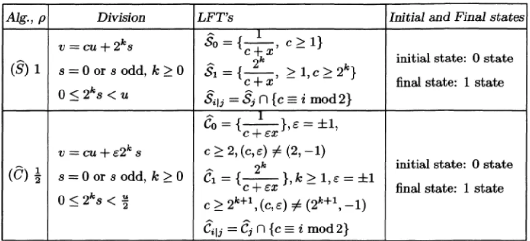
we describe the costs that will be studied.

2.1. Two Euclidean

_Algorithms.

The standard Euclidean division of

v

by

u

(v &#x3E; u),

of the form v = _{au +}

r,

produces

a

_positive

remainder r

such that 0 r ~. The centered division between u and v

(v &#x3E;

u/2),

of

the form v = _{au +}

Er,

produces

a

_positive

remainder r such

that 0 r

_u/2.

A Euclidean

_algorithm

is associated to each

_type

of

division,

and

_they

are

_respectively

called the Standard

Algorithm

(8)

and

the Centered

_Algorithm

_(C).

We denote

_by

_£(z)

the number of bits in the

_binary

_{representation}

of the

positive integer

x, so that

t(x)

= 1.

Then,

the bit-cost of _a

division

_step,

of the form v = _au is taken to be

essentially

£(u)

x

_{£(a) ,}

a

_quantity

that we

_adopt

as our

bit-complexity

measure. 1

It is followed

by exchanges

which involve numbers u and _r, so that the total cost of a

step

is x

f(a) + f(u) + ~(r).

In the case of the centered

division,

there

is

_possibly

an additional subtraction

(in

the case

when c = -1)

in order to

obtain a remainder in the interval

[0, u/2].

When

_given

an

_input

(vi, vo),

both

_{algorithms perform}

a certain number _p

of divisions of the form

and

_decomposes

the rational x =

(vl/vo)

as

(vl/vo)

=

h,

_o

h2

₀

... o

hp (0),

where the

_hi’s

are linear fractional transformations

(LFT)

of the

form hi

=

with =

1 /(a

₊

dx).

The

_pair

_{m :=}

(a, d)

is called the

digit-pair

of the LFT. The

_algorithm

then

_computes

the continued fraction

expansion

of rational x =

(vi/vo),

(CF-expansion

for

short),

In both _cases, the last non-zero

_integer

_vp is the

_gcd

of the

_pair

(vl, vo).

The

precise

form of the

_possible

LFT’s

_depends

on the

specific

algorithm;

there

exists a

special

set .~ of LFT’s in the final

_step.

However,

all the other

_steps

use the same set of LFT’s that is denoted

_by

1í. For the centered

_algorithm

(C),

the rational

_belongs

to Z =

~0, 1/2~;

for the standard

algorithm

(S),

the rational x

belongs

to I =

~0,1~.

Altogether,

the rational

inputs

of each

algorithm belong

to the basic interval I =

[0, p]

with _p = 1 _or

p =

1/2.

2.2.

_{Bit-complexities}

related to Euclidean

_Algorithms.

In both

cases, when

performing

p divisions on the

_input

(vl, vo),

the bit-cost

C(vl, vo)

of the

_algorithm

is a sum of _p

_terms,

the i-th term

represent-ing

the cost of the i-th division and

_being

a

_product

of two

_factors;

the first factor involves the

_binary

_length

_{£(vj )}

of

_{integer vj (with j}

_{possibly equal}

to i or i +

1),

while the second one involves a cost relative to the i-th LFT

to be

_performed,

of the form

_c(hi),

or of the form

c(mi),

where _mi is the

digit-pair

that defines the LFT

_hi.

In the

_sequel

_(see

Remark at the end of Section

_4),

we will see that we can

replace

the

length

e(v)

of

_{integer v by}

its

_logarithm

_log2(v)

in base 2 and

_{systematically}

consider

_log2(vi)

as the

first factor to be studied. In

_contrast,

we have to work with the exact cost

FIGURE 1. The Euclidean

_algorithms.

of the

_algorithm

on the

_input

(vi, vo)

will be of the form

IY1

The array of

_Figure

1 describes the

_precise

forms of the

_divisions,

the

_generic

set x of associated

_LFT’s,

the final set ,~ and the cost of the LFT’s.

It is also

_quite

useful to describe the

_{bit-complexity}

of so-called Extended Euclidean

_Algorithms,

that

_compute

at the same time Bezout coefficients of

pair

(vl,

vo),

i.e., integers

r and s such that rvo+svl =

gcd(vi, vo)

=

vp. The

principle

is

_well-known,

and the

_computation

makes use of two

_auxiliary

sequences ri

and si

that

satisfy

for each index i the relation rjvo + sjvi =

vi,

so that for i =

p, the Bezout relation holds with r := _{rp and} s := _{sp. The} sequences are initialized as ro =

l, so

=

O, r1

=

0, SI

=

1,

then

they

_are

built with the

_help

of _{sequence ai,}

in the same _way as the _sequence vi. The

supplementary

bit-cost due to

the extension of the

_algorithm

is thus a sum _terms, the i-th term

representing

the cost of the two

_{multiplications}

of the i-th

_step

described in

(4),

and

_being

a

product

of two

_factors;

the first factor involves the

_binary

lengths

of

_integers

_{ri, Si} while the second one involves a cost

c(m2)

relative to the i-th

_digit-pair

mi :=

(ai, di).

Finally,

for the same reasons as

_previously

(that

we shall

_explain

at the end of Section

_4),

the studied bit-cost

_{D(vi, vo)}

of both Extended

_algorithms

on the

_input

(vl, vo)

will be of the form

where the cost is defined in

_Figure

1.

We are

finally

interested in

_describing

the

length

of the

_binary

word that

encodes the

_pair

_{(vl, vo).}

There are two _ways for

_coding

this

_pair:

the first

the second one deals with the

binary encoding

B(vl, va)

of the _sequence of

digits

(ml,

m2, ... ,

mp).

It is

important

to compare the average

length

of

these two

_coding

_{words, since,}

in some

applications

that use

CF-expansions

in an extensive way, it may be useful to encode

_efhciently

the _sequence of

CF-digits,

so that this

encoding

can be

directly

used in further

computa-tions. Classical results in Information

_Theory

entail that the mean value

of

_{B(vl, vo)}

is at least

_equal

to the mean value of

A(vi,

vo).

This leads us

to

_study

the

_length

of the

_CF-encoding

of a

_pair

(vl, vo),

related to some

_digit-cost

_c, as well as to

_try

and find

_near-optimal

encod-ings.

2.3. Main

_parameters

for the

_analysis

of Euclidean

_Algorithms.

The costs to be

_studied,

defined in

_{(3), (5), (6),}

involve five main

param-eters : the

_integer

_p, the costs

_c(m)

of

_digit-pairs,

and the

_logarithms

of

integers v2

defined in

_(1),

_together

with the

_logarithms

of

_integers

_[

defined in

_(4).

The first

_parameter

is

_exactly

the

_depth

of the continued fraction

_expansion

of

_vllvo,

or the number of divisions to be

_performed

_by

the

_algorithm

on

input

(vi, vo).

Its _average behaviour is now well-known.

The cost

_c(m)

of the

_digit-pair

m =

(a,

d)

may involve the

digit

a alone or the

digit d alone,

or both. More

generally,

it is

_interesting

to

_study

the random behaviour of other functions of

_digit-pair

m =

(a, d).

Finally,

the

_integers

are related to continuants. When one

_"splits"

the

_CF-expansion

₍₂₎

of

_{vi /vo}

at

_depth

_z,

one obtains two

_{CF-expansions}

/B

defining

a rational number: the left

_part

defines the

_"beginning

rational"

of the form

while the

_right

_part

defines the

_"ending

rational" of the form

The

_beginning

rationals

_pi/qi

are useful for

_{approximating}

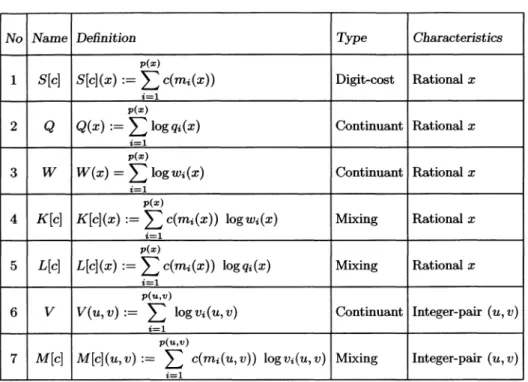
the rational

FIGURE 2. The main costs to be studied.

continuants.

_They

are

_closely

related to _{sequences ri}

_{and si}

that _appear

in the Extended Euclidean

_Algorithms,

via the relations _{pi =}

The

_ending

_{continuants, i.e.,}

the denominators wi of the

ending

rationals are

_closely

related to the

_{integers vi}

that _appear in the execution

₍₁₎

of Euclidean

_algorithm

on

_input

vl /vo,

via the

relation v2

=

w2.

When

_given

a valid

input

(u, v)

relative to some Euclidean

Algorithm,

we

wish to

_study

the behaviour of seven

_quantities,

that

fully

describe the cost

relative to some

_parameter

_during

the execution of a Euclidean

_Algorithm

on

input

(u, v) .

These

quantities

define what we call

_generic

costs and are

listed in

_Figure

2.

The first five

_quantities

_(1-5)

of

_Figure

2 are

_expressed

_only

in terms of

depth,

digits

and continuants. Since the

_depth

_p, the sequence of

digit-pairs

mi -

(ai, di)

and the sequence of continuants qi or _wi

_only

_depend

on rational x :=

(u/v)

and not on the

pair

(u, v)

itself,

these

_quantities

define functions of the rational x =

(u/v) .

The first _one is relative to _some

digit-cost

defined on the _sequence of

digit-pairs

_{ml, m2, ...} that _appear

in the continued fraction

_expansion

of x. The second and the third ones

are relative to

_(beginning

or

ending)

continuants,

and the fourth and fifth

or _q2. All these costs can also be viewed as functions defined on

pairs

on

integers

that we denote in the same _way,

Finally,

the last two

_quantities

_(6-7)

to be studied involve the _sequence of

_{integers vi}

that _{appear in} the execution of Euclidean

_{Algorithm. They}

depend

on the

pair

(u,

v)

itself,

not

_only

on the ratio

(u/v)

but also on the

gcd

r(u, v).

The relation between vi and Wi,

i.e.,

vi(u, v)

=

r(u, v) wj (u, v)

entails that V and

_M[c]

are

respectively

related to W and

_K(c~,

2.4.

_Average

values of costs.

_{Here, I}

denotes the basic interval. We consider the

_following

sets

for the

_possible

_inputs

of a Euclidean

_algorithm.

Remark that set

_QN

can

be viewed as the set of irreducible rationals with denominator less than N.

We denote

_by

_{X (u,}

_v)

one of the

_generic

costs that are defined in

_Figure

2.

We wish to

_study

the mean value of X on

QN

and

ON

that we denote

by

EN[X]

or

EN ~X ) .

More

_precisely,

we aim to evaluate the

asymptotic

behaviour

_(for

N -

_oo)

of the mean values

We will _{prove in} the

_sequel

that it is sufficient to

_study

the first five costs

(1-5)

defined in

_Figure

2 that are relative to rational numbers. The next

section

_analyses

these costs when x is

_real,

and

_gives

some indications on

what can be

expected

in the rational case.

3. Continued Fraction

_{Algorithms. Symbolic Dynamics}

and

Ergodic

Theorems

We now relate Euclidean

_algorithms

with continued fractions

_algorithms

that can be viewed as continuous extensions of them. Continued fractions

algorithms

are

_{important particular}

cases of what is

usually

called

dynamics

concerns itself with the

interplay

between

_properties

of the

trans-formation and discrete

_properties

of

_trajectories

of

_points

under iteration of the transformation.

_There,

_ergodic

theorems are _very useful to

_study

the

main

_parameters

of

_interest,

when x is almost _any real of the interval.

We

_adopt

here an

analytic

point

of

view,

with

hypotheses

_stronger

than

usual,

which entails easier

_proofs

and is

_well-adapted

to continued fraction

systems.

3.1. Piecewise

_analytic

_maps of the interval.

_Here,

we restrict

our-selves to the

_particular

case where the transformation is

_piecewise

_analytic.

Definition 1.

_[Piecewise

_analytic

_maps of the

_interval]

Let I be a real

interval. A

_mapping

U : Z -~ I is

_{piecewise analytic}

if there exists a

(finite

or

_denumerable)

set

_As

whose elements are called

_digits,

and a

_partition

of the interval I in subintervals

_Ij

such that the function x ~ Ux maps

analytically

each

Ij

onto 1.

A

_{piecewise analytic}

_{map thus consists} of

_denumerably

_many branches

in-dexed

_by

some set .M. We let

_M(x)

E M

_represent

the

_{index j}

of the subinterval

_Ij

where x falls. A

_coding

of a real number x is then obtained

by

the _sequence of

_digits

of the successive iterates of _x,

Here powers denote

iteration, U2

= U o

_U,

_etc. The _{sequence of}

_digits

_of

x is then

produced by

the

_following

simple

_algorithm.

Procedure

_Expansion

_(x)

A

_special

role is

_{played by}

the set H of branches of the inverse function

U-1

of U that are also

naturally

numbered

by

the index set we denote

_by

the inverse of the restriction If Xk := and the _sequence

m =

(ml, ... ,

of the first k

_digits

are

_known,

the

_algorithm

can be run

backwards,

and the

_original

xo is recovered

by

The

_semi-group

:=

_{generated by}

H is the set of all finite

com-positions

o ... _o the

length

of the

_{decomposition}

of h is

called the

_depth

of h and denoted

_by

_lhl.

The scheme

₍₁₄₎

_generalizes

the usual

_{binary representation}

of real numbers and it constitutes also a _{very convenient} framework for a discussion of continued fraction

_algorithm.

3.2.

_Ergodicity

and

_Ergodic

Theorem. We recall here some classical

definitions cast in our

particular

framework.

Here,

I denotes a real interval

endowed with its

_Lebesgue

measure dt. We consider here another measure

ti with a continuous

density

_g, so that

d¡,t(t)

=

g(t)dt.

Definitions 2.

_{[U-invariant measure]}

Let U be a measurable

_mapping

U : Z - 1. The measure _ft is said to be U-invariant

_if,

for _any subinterval

one has

~c(U-1,7) _

[Ergodicity]

Let U be a measurable

_mapping

U : Z ~ I

and p

be a

U-invariant measure. The

triple

(I,

U,

is

ergodic if,

for _any subinterval

y C

I such that C

_,7,

one has = 0 _or 1.

[Strongly mixing]

Let U be a measurable

_mapping

U : Z -&#x3E; Z and _ti be a U-invariant measure. The

triple

(I,

U,

tt)

is

strongly

mixing if,

for _any

subinterval

_{:1, JC}

C

_I,

one has rl

Naturally,

the

_mixing

_property

_implies

the

_ergodic

_property.

Ergodic

Theorems relate two different kinds of means relative to a function

f :

the mean value of

f along

an orbit of the form

(x,

Ux,

UZx, ...

Unx, ... )

and the mean value of

_f

relative to measure _1L.

BirkhofF’s

_Ergodic

Theorem. Let

_(I,

_U,

_p)

be

_ergodic.

_Then,

for _any

f

E

£1(I),

one

_has,

for almost all x of

_1,

3.3.

_{Strongly expanding}

_maps of the interval and

_ergodicity.

Clearly,

the stochastic behaviour of a

_numbering

_system

is

_closely

related

to the

_dynamics

of _map U on the interval

Z;

this

_dynamics

is itself

iso-morphic

to the

_dynamics

of the

_semigroup

7~C* that is

_{generated by}

the

set H of inverse branches. We now consider an

_important

class of _maps

U for which this

_dynamics

is well understood: the case of the

_(strongly)

expanding

maps.

Definition 3.

_[Strongly

_expanding

_maps of the

_interval]

Let I be a real

interval,

and let U : Z ~ ~ be a

piecewise

analytic

_mapping

whose set of inverse branches is denoted

_by

~‘~C. The

_mapping

U is

_{strongly expanding}

if there exist an _open disk V whose closure contains the interval I and a real

a 2 such that the

_following

holds:

(a)

every h E 1t has an

analytic

continuation on

_V;

(b) h

maps the closure V of disk V inside

V;

(c)

For

_{any h}

E

_H,

the absolute value

lh’I [

of the derivative has an

analytic

(d)

For

_{any h}

E

_1t,

the _supremum

_J(h)

:= E

VI

satisfies

b(h)

1 and the series

_¿hE1-l

_converges.

Remark 1. The

_{quantity 6}

:=

sup {8(h), h

E

_?-L}

satisfies 6 1 and defines the contraction ratio. The _map U is called

_expanding

since the derivative satisfies

_(1/b)

&#x3E; 1. When there exists some

_integer

k &#x3E; 1 for which

Uk

is

_strongly

_expansive,

then U is called

_eventually

strongly expanding.

The

_triple

_(V,

_a,

₆₎

that intervenes in Definition 3 is

called the

_triple

of U.

Remark 2. The _map U is called

_strongly

_expanding

because of two

as-sumptions :

(i)

the various

_analytic

continuations of h and

_Ih’l

on some disk

V that

_strictly

contains interval

_Z~,

_(ii)

the fact that the real a is

strictly

less 2.

We state now the

important

and classical result that shows that a

_strongly

expanding

map of the interval is

strong

mixing

(and

thus

_ergodic)

with

respect

to its

_(unique)

invariant measure.

Theorem. Let U be an

_{eventually strongly}

_expanding

_map of Z. Then

there is a

unique

U-invariant measure _JL.

Moreover,

the

triple

(I,

U,

~,)

is

strongly

mixing

(thus ergodic)

and the measure _{p is} of form

_{dp =}

0(t)dt

where 0

is

_analytic

on the

neighborhood

V of 1.

The main tool used in the

_proof

is the Perron-Frobenius operator that we now introduce.

3.4. The Perron-Frobenius

_operator

relative to a

_strongly

ex-panding

map. As

previously,

the set 1t denotes the set of inverse branches of U. The Perron-Frobenius

_operator

H relative to

_1t,

_together

with its

component operators

Rh

relative to each inverse branch

_h,

is defined as

follows:

First,

the _operator H is a

_{density transformer, i.e.,}

Second,

the n-th iterate of H describes what

_happens

_during

the n-th iter-ation of

_mapping

U.

_{Multiplicative properties}

of the derivative entail that

the n-th iterate of H involves all the inverse branches of

_{depth n,}

If U is

_{strongly expanding,}

we can _prove the

following.

Denote

by

the set formed with functions

_f

that are

_analytic

on V and continuous on

V.

Endowed with the _sup-norm, this set is a Banach _space and each

com-ponent operator

Rh

is a

_composition

_operator.

This

_type

of

_operators

was

extensively

studied

_{by Shapiro}

_[33]

who proves

that,

under

assumptions

(a), (b), (c),

they

act on are

_compact,

and even nuclear in the sense

of Grothendieck

_{[17, 18].}

Under condition

_(d),

the

operator

H itself acts

on is

_compact

and nuclear.

_Furthermore,

the

_operator

H has

pos-itive

_properties

that entail

_(via

Theorems of Perron-Frobenius

_type

due to

Krasnoselsky

[24])

the existence of dominant

_{spectral objects:}

there exist

a

_unique

dominant

_eigenvalue

A

_strictly

_positive,

a dominant

_{eigenfunction}

denoted

_by

_strictly

_positive

on VnR and a dominant

_projector

E. Under

normalization condition =

1,

these last two

objects

_are

unique

too.

Then, compacity

entails the existence of a

spectral

_gap between the

dom-inant

_eigenvalue

and the remainder of the

_spectrum.

Since H is a

density

transformer,

the dominant

_eigenvalue

satisfies A = 1 and the dominant

pro-jector

satisfies

_E[f]

_{= II f(t)dt.}

Then the dominant

_{eigenvector 0}

is also

an invariant function under H and the _{measure 1L} defined as

dp(t) = (t) dt

is U-invariant.

_Finally,

the

_{decomposition}

where the

_operator

N relative to the remainder of the

_spectrum

_(cf

a

_precise

definition in

_[27])

has a

_spectral

radius

_strictly

less than

_1,

_proves that

with

_{exponential speed,}

_{and 7p}

is also the the limit

_density

on I when _map

when

_applied

_{to g}

_{:= 13 ’ljJ}

and

_f

_:=1~

for some subintervals entail

that measure p defined

by

:=

qp(t)dt

is

_strong

_mixing

(with

exponen-tial

_speed)

and thus

_ergodic.

Remark. We

only

need in the

_previous

_proof

a weak form of condition

(d),

i.e.,

the fact that the series

_¿hE1-l

_converges for a = 2.

However,

the

_strong

form of condition

_(d)

_{(i.e., ~}

₂₎

will be

_{quite important}

for the

_{sequel, particularly}

in Section 4.5.

3.5. Some

_important

_asymptotic

mean values. Since

function 0

is

also the limit

_density

on Z~ when the _map U is iterated _many

_times,

the mean

values relative

_{to p}

can be also considered as

_asymptotic

mean values and

denoted

_by

_{Eco. Here,}

we

_give

some

_{important asymptotic}

mean values

that

_{play a}

central role in the

_{sequel. They}

are relative to

_digits

or to

entropy

of the

_dynamical

_system.

If M denotes the

_numbering

_function,

and c denotes a

cost-digit

function c : .ll~I -~

R+,

then the

asymptotic

mean value of c o M is

The

_entropy

of the

_dynamical

_system

is defined as the

limit,

if it

exists,

of a

_quantity

that involves _{measures ug} of intervals

g(Z), (for g

E

_71*)

Via a classical formula due to

_Rohlin,

the

_entropy

is related to the

asymp-totic mean value of

log

lU’l

[

In the

_sequel,

we describe the numeration

_systems

relative to continued

frac-tions,

the standard continued fraction

_system

and the centered continued fraction. In both _cases, we obtain real extensions of Euclidean

_algorithms

that

_give

rise to

_expanding

_maps where the

_ergodic

framework can be used.

3.6. Standard and centered continued fraction

_expansions.

The

continued fraction

_systems

fit into the

_general

framework of

_piecewise

integer

part

function denoted

_{by x ~}

_{l x J}

and the fractional

_part

function

~ 2013~ := x - It is described

by

the

quadruple

(I,

U,

_m,

H)

We also let

_U(0)

=

0,1/0

= 0. Centered continued fractions _are obtained

when one

_replaces

truncation

_(integer

_part

_function)

_{by rounding}

to the

nearest

_{integer x --&#x3E;}

_~~x~~.

First introduce the notations

so that the

following identity

holds:

Then,

the centered continued fraction

_system

is defined

_by

the

_quadruple

(I,

U,

m,

1(,)

given

by

with,

conventionally,

U(o)

=

0,

m(O)

=

0,

1/0

= 0.

These numeration

_systems

_provide

a _sequence of

digits according

to scheme

(14)

and thus continued fractions

_expansions,

that are

_generally

infinite.

When

_applied

to a rational _x, these

_expansions

are finite and coincide

with continued fraction

_expansions

of Section 2. In this _sense, continued fractions

_systems

can be viewed as extensions of Euclidean

_Algorithms,

and

in both _cases, the rational numbers are

exactly

the real numbers for which

the continued fraction

_expansion

is finite. A number x is rational if and

only

if there exists an element h of the

semi-group

H* for which x =

h(o).

3.’l.

_Applications

of

_Ergodic

Theorem to continued fractions

sys-tems. It is clear that both continued fraction

_systems

are related to

(even-tually)

strongly expanding

maps.

Then,

the

Ergodic

Theorem

applies

to

CF-expansions,

and classical results entail that the invariant measure _{it is}

of the form

_{dp(t) =}

with

The first result was

_{conjectured by}

Gauss,

then _proven

_by

_Levy

[26].

The

second result was established

by Rieger

[30].

The related distribution

We consider now some

_asymptotic

mean values that

_{play a}

central role in

the

_sequel.

The

_following

results are classical and can be found for instance in

_[5].

Digit-costs.

Consider some

_particular

digit-cost

c :

R+

such that

c o M is in If

_c(m)

_equals

for instance the

_binary

_length

of

_digit

_a,

_i.e.,

the number of

_{binary digits}

in the

_binary

_expansion

of

_digit

_c~, one

has,

with

_general

formula

_(20),

In the case of centered continued

fractions,

when

digit-cost

equals

the

sign

e, one obtains

-11 -11 ,

Then

_Ergodic

Theorems _prove

_that,

in both _cases, and for almost all x in

-T,

Entropy.

The variable x -&#x3E; ~

log

z

is

_{quite important}

_too, since the

asymp-totic mean value

_Eco

[I

_log

xl]

is

_closely

related to the

_entropy

_h(H)

of the

dy-namical

_system,

via Rohlin’s formula

₍₂₁₎

and the fact that

_IU’(x)1

₌

_1/x2,

so that

_explicit

values of

_entropy

are obtained in both _cases,

Continuants. This mean value intervenes also when

_studying

the _average

behaviour of the

parameter

log qn (x)

relative to

_(beginning)

continuant

qn (x)

that is well-defined for a

general

real number too. A real number

x whose continued fraction

_begins

with h =

hl

o

_h2

o ... o

hn

satisfies

x =

h(y)

=

hl

_o

h2

_{o ... o} with some y _E

I;

We relate x _to the

rational xo :=

h(O)

=

hl

o

_h2

0 ... o and the transforms

o

_h2

0 ... o to the transforms

_uj(xo)

=

The classical relation between numerator

_{pj (x)}

and denominator

_i.e.,

= _proves that

Since U is

_expanding

with contraction-ratio

_6,

one obtains an

_approximate

expression

of

_logqn(x)

that involves transforms

_logU2(x)

instead of

trans-forms

_log

_Ui(xo):

Since one has

there exists some constant K for

_which,

for any x, and any

integer

n,

Now,

the

_Ergodic

Theorem

₍₁₅₎

_applies

to the function

_log

_implying,

via

₍₂₅₎

and

_(26),

that

Relations between

_entropy

and mean

_{binary length}

of

_digits.

The

asymptotic

mean value relative to the

_binary

_length

and the

quan-tity

h(-H)/(2

log

2)

are

_related,

since the second one is the

_integral

of

11092 tl

[

with

_respect

to

_ergodic

measure, while the first one is the

integral

of the

function that

_equals

_llog2aJ

+ 1 on the interval We then obtain

the relation

3.8. Heuristic transfer from continuous model to discrete one.

With _respect to

_{asymptotic properties}

of continued

_fractions,

rational

num-bers are _very

_particular

since their continued fraction

_expansion

is finite.

However,

let us

_imagine

that continued fractions of rational numbers and

continued fractions of real numbers behave in the same _way and let us

suppose that the

Ergodic

Theorem may be

applied

to rational numbers

behaviours for our

_parameters

of interest relative to rational numbers and defined in

_Figure

2

However,

it is

_{highly probable}

that this result may be true

_only

_{in average}

on the set

_QN

defined in

₍₁₂₎

when N tends to oo. On the other

hand,

the

_depth

_p(x)

of a rational x of denominator N

equals

the rank n for

which

_equals

N. If rational numbers of

_large

denominator behave like

_generic

real

_numbers,

it is thus

_plausible,

from

_(27),

that

(2/h)

log

N for

_large

N. This is a well-known result for which we shall

give

an alternative

proof

in the

sequel.

Finally,

the

following

estimates are

plausible:

and will be proven in the

sequel.

4.

_Generating

_functions,

_dynamical

_operators

and Tauberian Theorems

Here,

we describe

_general

tools for

_analysing

the main costs of interest rel-ative to

_algorithms

of the Euclidean

_type.

We first introduce the Dirichlet

generating

functions relative to

_costs,

so that the _average cost involves par-tial sums of coefficients of these Dirichlet series. Tauberian Theorems are a classical tool that transfers the

analytical

behaviour of a Dirichlet series near its

singularities

into an

_asymptotic

form for its coefficients.

Then,

when

_viewing

the

_algorithm

as a

dynamical

_system,

we relate

generating

functions of costs to the Ruelle

_operator

associated to the

_algorithm,

so

that we can

_easily

describe the

_{singularities}

of

_generating

functions.

Fi-nally,

we _prove the estimates of the mean values that have been

previously

proposed

for the main

_parameters

of

_algorithms.

4.1.

_Generating

functions. We recall that we consider the

following

sets

as

possible

inputs

of a Euclidean

_algorithm.

Our _{purpose is} to estimate

and

QN-

More

_precisely,

we aim to determine

_{asymptotically}

_(as

N -

_oo)

these mean

values,

denoted

by

EN []

or

EN (X ~ ,

that

satisfy

The

_following

Dirichlet

_generating

functions of

_costs,

are of the form

where

_{an, an}

are the number of

pairs

(u, v)

of Q or Q with fixed v =

n, and xn,

xn

are the cumulative values of X on

_pairs

(u, v)

of Q or Q with fixed

v =

n, so that the _average costs in

₍₂₉₎

to be studied

are

_exactly

the

_quotient

of

_partial

sums of the coefficients of the Dirichlet

series defined in

_(30).

First,

remark that there is an _easy relation between

Gx

and

GX

when cost

X satisfies

_{X (u, v)}

=

X (au,

av)

for

any

integer

a &#x3E; 1. Then

where

_((s)

is the Riemann Zeta-function

This is the case when X = 1 _or when X is _one of the first five costs of

interest defined in

_Figure

2. For the last two costs defined in

_Figure

2 that involve

_integers

_vi, relations

₍₁₀₎

entail that

4.2. Tauberian Theorems. In the remainder of the paper, we aim to

apply

the

_following

Tauberian Theorem to the Dirichlet series

_{F, G x}

defined

in

₍₃₀₎

in order to estimate their coefficients.

Tauberian Theorem.

_[Delange]

Let

_F(s)

be a Dirichlet series with non

negative

coefficients such that

_F(s)

_converges for

_R(s)

&#x3E; (1 &#x3E; 0. Assume that

(i)

F(s)

is

_analytic

on

_R(s)

=

Q, s ~

_a, and

F(s)

=

A(s) (s -

~)-7-1

₊

C(s),

where

A,

C

are

analytic

_{at a,} with

A(Q) ~

0.

Then,

as N --&#x3E; _oo,

We first examine the case of functions

F(s),

F(s)

that are

_closely

linked to

the Riemann series

_~(s)

via the

_equalities

Then,

classical

_properties

_{of (}

function entail that the Tauberian Theorem

applies

to

_F(s)

and

_F(s),

with Q = 2

and

= 0. More

precisely,

at s =

2,

one has:

(s - 2)F(s) -

(6p)/7r~.

When X is one of the three costs defined in

_Figure

2 relative to continuants

Q, V,

W,

it

_applies

to with Q = 2

and I

=

3,

_so that the _mean value

EN [X]

will be of order

_log2

N. When X involves a

_digit-cost

_c, we will

exhibit some sufficient conditions on cost c under which the Tauberian

Theorem

_applies.

In this _case, the values Q

_{and -y strongly depend}

on

properties

of the

_digit-cost

c. In the case when c

equals

the

binary

digit-length

l,

the mean value

]

will be of order

_logN,

while the

mean-value will be of order

_log2

N. We can deal with varied

_costs;

for

_instance,

if

_c(m)

=

m log 2 m,

then

EN[S[c]]

is of order

log4

N,

and if

c(m)

=

T723~2~

then

EN[S[c]]

is of order

v’N.

It is not a

_priori

clear how to

_{directly apply}

Tauberian Theorems to

_{Gx (s).}

In the

_following,

we obtain alternative

expressions

for from

which the location and the nature of their

_{singularities}

will become

appar-ent. Our

_analysis

involves suitable Ruelle

_operators

that can be viewed as

extensions of

_density

transformers of Section 3.4 when one introduces some

complex

parameter s that

_plays

the same role as

_temperature

in statistical

mechanic.

4.3.

_Algebraic

_properties

of Ruelle

_operators.

The Ruelle

_operators

that we use now can be viewed as extensions of the Perron-Frobenius

The Ruelle

_operator

_Rs,h

relative to a LFT h

depends

on some

_complex

parameter s

and is defined as

where

_D[h]

denotes the denominator of the linear fractional transformation

(LFT)

h,

defined for

_{h(x) =}

_{(ax + b) / (cx + d)}

with a,

b,

c, d

coprime integers

by

D~h](x) :

:= =

Then,

for a LFT h of

determinant

_1,

the

_operator

_Rs,h

is an extension of the

_operator

Rh

defined

in

_(16),

via the

_equality

_R2,h

=

Rh.

Once a cost function c relative to the LFT h has been

_fixed,

one can define

another Ruelle

_operator

relative to

_h,

Now, given

an

_algorithm

and a set 1t of LFT’s used in one

_step

of the

algorithm,

the Ruelle

_operators

relative to 7~C are defined

by

As

_previously,

if the set ?nC is formed of LFT’s with determinant

_1,

the

operator

Hs

is an extension of the

_operator

H defined in

(16),

via the

equality

H2

= H.

In all _cases, the

_{multiplicative}

_property

of denominator

_{D, i.e.,}

D (h) (g (x) ) D ~g~ (x)

is translated into a

_{multiplicative}

_property

on Ruelle

operators:

Given two

_{LFT’S, h}

and g, the Ruelle

operator

associated

to the

_{LFT h o g}

is

_exactly

the

_operator

o

_Rs,h.

More

_generally,

when

given

two sets of

_LFT’s,

,C and JC and their Ruelle

_operators

_{Ks, Ls,}

the

set is formed of

_{all h o g}

with h E L

and g

E

_JC,

and the Ruelle

operator

relative to the set is

_exactly

the

_operator

_{Ks oLs .}

In

_particular,

the Ruelle

_operator

relative to the

_semi-group

?-~* := is

exactly

(I -

Hs)-1.

It is the

_{quasi-inverse}

of the Ruelle

_operator

_H,

associated to the set ~-L.

4.4. Ruelle

_operators

and Dirichlet

_generating

functions. We show

now how the Ruelle

_operators

associated to the

_algorithms

intervene in the evaluation of the

_generating

functions of costs

_{Gx (s),}

GX (s).

We recall that it is sufhcient to

_study

_GX

for one of the first five costs of

_Figure

2.

We consider here a Euclidean

Algorithm

and its set of LFT’s H

_together

with its final set J’ defined in

_Fig.l.

The Ruelle

_operators

_Hs,

_FS,

relative to ?~ or 7 and defined in

(33,

34,

35)

will

play a

central role in the

An execution of the

_algorithm

on the

_input

(vi, vp)

of S2

_performing

_p

_steps

of the form

decomposes

the rational as

(vi /vo)

=

hi

o

h2

0 ... o

_{hp (0),}

where the

h2’s

are elements of 1t

(for

i _{p -}

1)

or elements of ,~’

(for Z

=

p) .

The choice of an

index i,1 i

_p,

splits

the LFT h =

hl

_o

h2

₀

... o

hp

into

three different

_parts:

the

_beginning

_part

_{bi (h)}

:=

hl

o

_h2

0 ... o

_hi-1,

the

ending

part

ei (h)

:= o 0 ... o

hk,

and

finally

the i-th

_component

hi.

From

₍₈₎

and

₍₉₎

the

_following

_equalities

hold:

The derivative functional A

_plays

an

_important

role too. For some

op-erator

_Ls

that

_depends

on

_parameter

_s, the

_operator

AL,

is defined

_by

AL,

When

_applied

to defined in

_(33),

this functional A

is well-suited to the

_problem

since it

_produces

at the numerator the

loga-rithm

_logD[h].

When

_applied

to or to it

_produces

at the

numerator, via

_(36),

the

_beginning

or the

ending

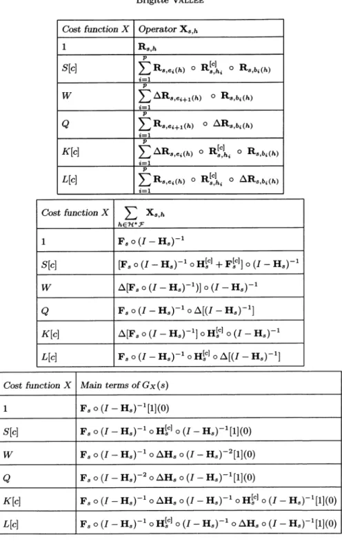
continuants.

We now introduce our main

_operators,

that are all built

_according

to the

same

principles:

each of them is

precisely

related to one of the

_generic

costs

X defined in

_{Figure 2,}

and the

_generic

_operator,

relative to

_generic

cost

_X,

is denoted

_by

_{Xs,h .}

If h is a LFT of

depth

_p, it is

expressed

as a sum of

p terms each of which may involve , Z ( ) and s,h2

however,

the

_precise

form of

_depends

on cost X .

_Figure

3

_(top)

describes the

operators

relative to the studied costs.

We claim

_that,

when

_applied

to function

_f

= 1 and

point x

=

0,

each

operator

Xs,h

generates

the cost

_vo)

of the

_algorithm

on

_input

(vi, vo)

of Q

Now,

when

_(vi,

_vo)

is a

general

element of

S2,

the LFT h defined

by

(2)

is a

general

element of set

_?~*,~,

so that we obtain alternative

_expressions

of our main Dirichlet series

_{F, G x}

defined in

₍₃₀₎

When index i varies in

_[l..p],

_beginning

_part

_bi(h)

is a

general

element of

H*, ending

part

ei (h)

is a

_general

element

of1t* F,

while the i-th

_component