On the application and interpretation of Keeling plots in paleo climate research ? deciphering ?<sup>13</sup>C of atmospheric CO<sub>2</sub> measured in ice cores

(1)

HAL Id: hal-00297805

https://hal.archives-ouvertes.fr/hal-00297805

Submitted on 14 Jun 2006

HAL is a multi-disciplinary open access

archive for the deposit and dissemination of sci-entific research documents, whether they are pub-lished or not. The documents may come from teaching and research institutions in France or abroad, or from public or private research centers.

L’archive ouverte pluridisciplinaire HAL, est destinée au dépôt et à la diffusion de documents scientifiques de niveau recherche, publiés ou non, émanant des établissements d’enseignement et de recherche français ou étrangers, des laboratoires publics ou privés.

On the application and interpretation of Keeling plots in

paleo climate research ? deciphering ?13C of atmospheric

CO2 measured in ice cores

P. Köhler, J. Schmitt, H. Fischer

To cite this version:

P. Köhler, J. Schmitt, H. Fischer. On the application and interpretation of Keeling plots in pa-leo climate research ? deciphering ?13C of atmospheric CO2 measured in ice cores. Biogeosciences Discussions, European Geosciences Union, 2006, 3 (3), pp.513-573. �hal-00297805�

(2)

BGD

3, 513–573, 2006 Deciphering δ13C of atmospheric CO₂ measured in ice cores P. K ¨ohler et al. Title Page Abstract Introduction Conclusions References Tables Figures J I J I Back Close

Full Screen / Esc

Printer-friendly Version Interactive Discussion

Biogeosciences Discuss., 3, 513–573, 2006 www.biogeosciences-discuss.net/3/513/2006/ © Author(s) 2006. This work is licensed under a Creative Commons License.

Biogeosciences Discussions

Biogeosciences Discussions is the access reviewed discussion forum of Biogeosciences

On the application and interpretation of

Keeling plots in paleo climate research –

deciphering δ

13

C of atmospheric CO

₂

measured in ice cores

P. K ¨ohler, J. Schmitt, and H. Fischer

Alfred Wegener Institute for Polar and Marine Research, P.O. Box 12 01 61, 27515 Bremerhaven, Germany

Received: 21 February 2006 – Accepted: 9 March 2006 – Published: 14 June 2006 Correspondence to: P. K ¨ohler (pkoehler@awi-bremerhaven.de)

(3)

BGD

Full Screen / Esc

Abstract

The Keeling plot analysis is an interpretation method widely used in terrestrial carbon cycle research to quantify exchange processes of carbon between terrestrial reservoirs and the atmosphere. Here, we analyse measured data sets and artificial time series of the partial pressure of atmospheric carbon dioxide (pCO₂) and of δ13C of CO₂over

5

industrial and glacial/interglacial time scales and investigate to what extent the Keeling plot methodology can be applied to longer time scales. The artificial time series are simulation results of the global carbon cycle box model BICYCLE. Our analysis shows that features seen in pCO₂ and δ13C during the industrial period can be interpreted with respect to the Keeling plot. However, only a maximum of approximately half of the

10

signal can be explained by this method. The signals recorded in ice cores caused by abrupt terrestrial carbon uptake or release loose information due to air mixing in the firn before bubble enclosure and limited sampling frequency. For less abrupt changes as occurring during glacial cycles carbon uptake by the ocean cannot longer be neglected. We introduce an equation for the calculation of the effective isotopic signature of

long-15

term changes in the carbon cycle, in which the ocean is introduced as third reservoir. This is a paleo extention of the two reservoir mass balance equations of the Keeling plot approach. Steady state analyses of changes in the terrestrial and marine biosphere lead to similar effective isotopic signatures (−8.6‰) of the carbon fluxes perturbing the atmosphere. These signatures are more positive than the δ13C signals of the sources,

20

e.g. the terrestrial carbon pools themselves (∼ −25‰). In all other cases the effective isotopic signatures are larger (−8.2‰ to −0.7‰), and very often indistinguishable in the light of the uncertainties. Therefore, a back calculation from well distinct fluctuations in pCO₂ and δ13C to identify their origin using the Keeling plot approach seems not possible.

25

(4)

BGD

Full Screen / Esc

1 Introduction

In carbon cycle research information on the origin of fluxes between different reser-voirs as contained in the ratio of the stable carbon isotopes13C/12C has become more and more important in the past decades. These isotopic signatures store information about exchange processes because differences in physical properties of atoms and

5

molecules containing different isotopes of an element lead to isotopic fractionation. Prominent examples in our context of global carbon cycle research are gas exchange between surface ocean and atmosphere or photosynthetic production in both the ma-rine and the terrestrial biosphere. Here, the end member of a carbon flux associated with a given process is in general depleted in the heavier isotope. This is expressed

10

with the fractionation factor ε of the process, which depends on various environmen-tal parameters such as temperature or the biological species (see Zeebe and Wolf-Gladrow (2001) for more basic information on carbon isotopes in seawater).

The isotopic composition of a reservoir is usually expressed in per mil (‰) in the so-called “δ-notation” as the relative deviation from the isotope ratio of a defined standard

15 (VPDP in the case of δ13C): δ13C_sample=    [13C] [12_{C] sample} [13_C] [12_{C] standard} − 1   × 10 3_. ₍₁₎

The fractionation factor ε (in ‰) between carbon in sample A and in sample B (e.g. be-fore and after some fractionation step) is related to the δ values by

ε_(A−B)= δ A

− δB

1+ δB_/103. (2)

20

During photosynthesis the carbon taken up by marine primary producers is typically depleted by −16 to −20‰. On land, the type of metabolism determines the fractionation factor during terrestrial photosynthesis. C₃plants inhibit a higher discrimination against

(5)

BGD

Full Screen / Esc

the heavy isotope (ε=−15 to −23‰) than plants with C₄metabolism (ε=−2 to −8‰) (Mook,1986).

One prominent interpretation technique of carbon exchange between the atmo-sphere and other reservoirs, e.g used in carbon flux studies in terrestrial ecosystems, is plotting the δ13C signature of CO₂ as a function of the inverse of the atmospheric

5

carbon dioxide mixing ratio (δ13C=f (1/CO₂)). In doing so, the intercept of a linear regression with the y-axis can under certain conditions be understood as the isotopic signature of the flux, which alters the content of carbon in the atmospheric reservoir. This approach is called “Keeling plot” after the very first usage by Charles D. Keeling about 50 years ago (Keeling,1958,1961). The application and interpretation of

Keel-10

ing plots is widely used in terrestrial carbon research and based on some fundamental assumptions (see review ofPataki et al.,2003).

Keeling plots have also been used in paleo climate research in the past years (e.g. Smith et al.,1999;Fischer et al.,2003), but it seems that the limitations of this approach have not been adequately taken into account to allow for a meaningful interpretation.

15

The aim of this paper therefore is to emphasise what can be learnt from Keeling plots, if applied on slow, but global processes acting on glacial/interglacial time scales, and to discuss their limitations. We emphasise what kind of information can be gained from deciphering the δ13C signal measured in ice cores. For this purpose we extent the Keeling plot approach to a three reservoir system and analyse data sets and artificial

20

time series produced by a global carbon cycle box model, from which we know which processes are operating.

2 The Keeling plot

The principle of the Keeling plot approach is based on the exchange process of carbon between two reservoirs and the conservation of mass. Let C_newbe the mass of carbon

25

(6)

BGD

Full Screen / Esc

after the addition of carbon with mass C_addto an undisturbed reservoir with mass C_old.

C_new= C_old+ C_add (3)

With δ13C_xbeing the carbon isotope signature of the C component x the conservation of mass thus gives us:

C_new· δ13_C

new= Cold· δ13Cold+ Cadd· δ13Cadd (4)

5

In combining Eqs. (3) and (4) we obtain a relationship between δ13C_newand C_new:

δ13C_new= C_old· (δ13_C old− δ13Cadd) · 1 C_new+ δ 13_C add (5)

Thus, the y-intercept y₀ of the linear regression function of Eq. (5), which describes

δ13C_newas a function of the inverse of the carbon content (1/C_new), gives us the isotopic ratio δ13C_add of the carbon added to the reservoir.

10

There are two basic assumptions underlying the Keeling plot method: (1) The system consists of two reservoirs only. (2) The isotopic ratio of the added reservoir does not change during the time of observation. Both assumptions are only rarely fulfilled. Fur-thermore, there are arguments about which linear regression model should be used if one assumes measurement errors in both variables (for details seePataki et al.,2003).

15

The methodological aspects concerning the choice of a regression model are not the subject of our investigations here.

The Keeling plot approach was used in the past to interprete various different sub-systems of the global carbon cycle. Keeling (1958, 1961) first used it to identify the contribution of terrestrial plants to the background isotopic ratio of CO₂in a rural area

20

near the Pacific coast of North America. Later, the component of the terrestrial bio-sphere in the seasonal cycle of CO₂over Switzerland (Friedli et al.,1986;Sturm et al., 2005) and Eurasia (Levin et al.,2002) was investigated with the Keeling plot. The ap-proach was widely used in terrestrial ecosystem research to identify respiration fluxes (e.g.Flanagan and Ehleringer,1998;Yakir and Sternberg,2000;Bowling et al.,2001;

25

(7)

BGD

Full Screen / Esc

Pataki et al.,2003;Hemming et al.,2005). It was used in paleo climate research within the last years to disentangle the processes explaining the subtle changes in CO₂ dur-ing the relatively stable LGM and the Holocene as well as the approximately 80 ppmv increase from the Last Glacial Maximum (LGM) to the Early Holocene (Smith et al., 1999;Fischer et al.,2003;Eyer,2004).

5

3 Global CO₂and δ13C times series of different temporal resolution

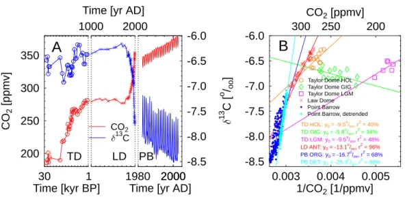
It has been shown (Fischer et al.,2003), that the seasonal amplitude of CO₂and δ13C during the last decades, the anthropogenic rise in CO₂ and the corresponding de-crease in its δ13C signal since 1750 AD, and the glacial/interglacial variation in these two records exhibit significant different behaviour if analysed with the Keeling plot

ap-10

proach. Data sets showing these dynamics on the three different temporal scales are compiled in Fig.1. The seasonal signal is measured from 1982 to 2002 AD at Point Barrow, Alaska (Keeling and Whorf,2005;Keeling et al.,2005). For the anthropogenic variation during the last millennium we use the data measured in air enclosures in the Law Dome ice core (Francey et al.,1999;Trudinger et al.,1999). Glacial/interglacial

15

variations (1−30 kyr BP) were detected in the Taylor Dome ice core (Smith et al.,1999). For the interpretation of the seasonal signal measured at Point Barrow both data sets (CO₂, δ13C) need to be detrended to separate the two simultaneous occurring effects of the anthropogenic CO₂rise and the seasonality from each other. Annual variations are then analysed as perturbations from the mean values during the first year of the

20

measurements. The component C_add in Eqs. (3)–(5) reflects the exchange of carbon of an external reservoir (winter time carbon release from the terrestrial biosphere in the seasonal signal of Point Barrow and anthropogenic emissions in the case of Law Dome) with the atmospheric reservoir. The Point Barrow and Law Dome data can be approximated consistently with the typical Keeling plot linear regression function

25

(r2=96% in both). The y-axis intercept y₀declines from the seasonal effects (−25‰) to the anthropogenic impact (−13‰) with the mixed signal of the untreated data at Point

(8)

BGD

Full Screen / Esc

Barrow in-between (−17‰) (Fig.1b). This decline is explained by a larger oceanic car-bon uptake and a smaller airborne fraction of any atmospheric disturbance in CO₂ in longer time scales (Fischer et al.,2003).

These two examples based on accurate data sets are already beyond Keelings orig-inal idea as they are no longer based on a two reservoir system and highlight the

5

limitations of this approach. While the y-intercept of the detrended data at Point Bar-row match the expectations well, the intercept found in the anthropogenic rise in Law Dome does not record the δ13C signal of the carbon released by anthropogenic activity (with δ13C of about −25 to −30‰) to the atmosphere anymore. The seasonal ampli-tude at Point Barrow can be explained with the seasonality of the terrestrial biosphere.

10

Vegetation grows mainly in the northern hemisphere, and thus CO₂minima occur dur-ing maximum photosynthetic carbon uptake by plants durdur-ing northern summer. The seasonal fluctuation in CO₂ should therefore bear a δ13C signal of the order of −25‰ which would account for fractionation during terrestrial photosynthesis (Scholze et al., 2003). This δ13C signal of the seasonal cycle is seen in the detrended Point Barrow

15

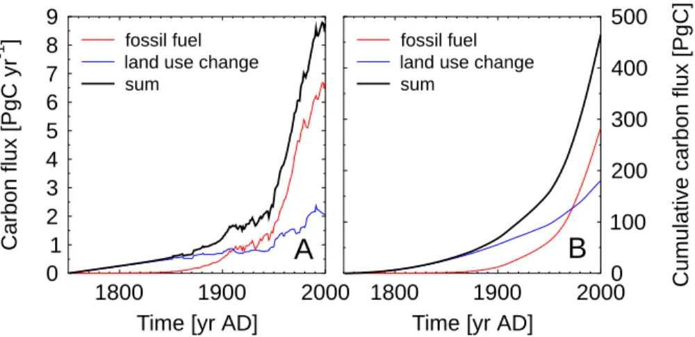
data and corresponds well with other studies (e.g. Levin et al., 2002). The anthro-pogenic rise seen in the Law Dome data set is the residual of the combination of fossil fuel emissions (Marland et al.,2005), land use changes (Houghton,2003), terrestrial carbon sinks due to CO₂ fertilisation (Plattner et al.,2002), all from which the ocean carbon uptake during that time has to be subtracted. Until about 1910 AD the fossil

20

fuel emissions were smaller than the carbon release caused by land use change (both around 0.8 PgC yr−1). The relation changed thereafter and in the year 2000 AD fossil fuel emissions were already more than three times larger than carbon fluxes based on land use change (6.7 versus 2.1 PgC yr−1; Fig. 2a). The cumulative release of fossil fuel carbon out-competed that from land use change only in year 1973 AD.

Al-25

together about 465 Pg of carbon were released by anthropogenic activities during this 250 year period to the atmosphere (Fig.2b). Without carbon uptake by the ocean and the terrestrial reservoirs this would have led to a rise in atmospheric CO₂by more than 200 ppmv. The δ13C signal of recent fossil fuel emissions in the USA is around −29 to

(9)

BGD

Full Screen / Esc

−30‰ (Blasing et al.,2004), while carbon fluxes from land use changes bear the typ-ical δ13C signal of the terrestrial biosphere (−25‰). These anthropogenic processes can by no means be deconvoluted by the Keeling plot analysis. The reason for this is that due to the gas exchange between ocean and atmosphere the basic assumption of a two reservoir system is intrinsically violated. This questions the applicability of

5

the Keeling plot approach to carbon change studies on long time scales, where this ocean/atmosphere gas exchange becomes even more significant.

Going further back in time, the glacial/interglacial rise in CO₂ and its accompanied

δ13C variations as measured in the Taylor Dome ice core led to a sub-grouping of the

δ13C–1/CO₂ data pairs (Smith et al., 1999) with different linear regression functions

10

for the Last Glacial Maximum (LGM), the glacial-interglacial transition (GIG), and the Holocene (HOL) (Fig.1b). With on average one data point every thousand years the data set is sparse. However, the y-intercepts during LGM and Holocene are similar (−9.5‰) and significantly different from that during the transition (−5.8‰). Thus, it was hypothesised that underlying processes for variations in CO₂during the relatively stable

15

climates of the LGM and the Holocene might have been the same and might have been mainly based on processes concerning the terrestrial biosphere (Smith et al.,1999; Fischer et al.,2003).

4 Extending the Keeling plot approach to a three reservoir system

A first estimate for the effective carbon isotopic signature in the atmosphere due to an

20

injection of terrestrial carbon into the ocean/atmosphere system can be derived when extending the two reservoirs to a three reservoir system. Here we assume that ocean circulation remained the same and that an equilibrium between ocean and atmosphere is achieved.

We have to extend the carbon and isotopic balance according to

25

A+ O = A₀+ O₀+ B (6)

(10)

BGD

Full Screen / Esc

and

AδA+ OδO= A₀δ₀A+ O₀δ₀O+ BδB. (7)

where A₀=600 PgC and O₀=38 000 PgC are the reservoir sizes of the atmosphere and ocean, respectively, before an injection of terrestrial carbon of the size B. A and O are the sizes of the atmospheric and oceanic reservoirs after the injection. The δ₀’s

5

represent the carbon isotopic signatures of the reservoirs before the injection with

δ₀A=−6.5‰ and δ₀O=+1.5‰ and the δ’s after the injection. The isotopic signature

of the terrestrial biosphere δB=−25‰ is assumed to be constant. Note, that during the gas exchange and the dissociation of carbonic acid in the seawater fractionation occurs (according to Eq.2) ε_AO≈δ₀A−δ₀O≈δA−δO≈−8‰, which is assumed to remain

10

constant in time.

For the oceanic uptake of carbon we have to take the buffering effect of the carbonate system in seawater into account (Zeebe and Wolf-Gladrow,2001). The ratio between the change in CO₂concentration and the change in dissolved inorganic carbon (DIC) is described by the Revelle or buffer factor β, which is temperature, alkalinity and DIC

15 dependent: β := d [CO2]/[CO2] d DIC/DIC ! . (8)

Any additional carbon injected into the ocean/atmosphere system will be distributed in the two reservoirs according to the ratio of the sizes before the injection, i.e.

A− A₀

O− O₀ = β

A₀

O₀. (9)

20

Using the carbon balance in Eq. (6) we can calculate the size of the ocean and atmo-sphere reservoir after the injection

O= βA0+ O0+ B

βA₀/O₀+ 1 . (10)

(11)

BGD

Full Screen / Esc

The Revelle factor β in recent surface waters varies between 8 and 16 (Sabine et al., 2004). For the preindustrial setting β in the surface ocean boxes of our box model BICYCLE is on average 11.5, with 9 in equatorial waters and around 12 in the high latitudes. Note that the average Revelle factor of the surface ocean falls to 10 for the climatic conditions of the LGM.

5

The effective carbon signature of the isotopic change in the atmosphere δ∆Acan be estimated according to δ∆A= Aδ A_{− A} 0δ A 0 A− A₀ . (11)

Using the carbon isotopic balance in Eq. (7) and replacing δO=δA−ε_AO we obtain

δ∆A= A0+O0+B−O A0+O0+B (A0δ A 0 + O0δ O 0 + Bδ B_{+ ε} AOO) − A0δ A 0 O₀+ B − O . (12) 10

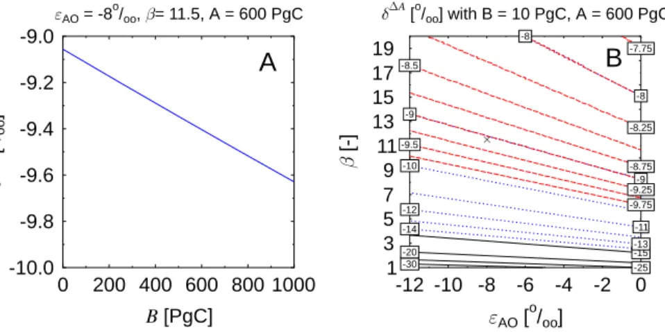
When we insert the values for isotopic signatures and reservoir sizes given above and vary the amount of terrestrial carbon added, the isotopic fractionation during gas ex-change ε_AO or the Revelle factor β we obtain varying effective isotopic signatures δ∆A of the change in the atmospheric carbon reservoir as shown in Fig.3. In a setting for the preindustrial climate conditions, δ∆Avaries nearly linear with B between −9‰ and

15

−10‰ (Fig.3a), reflecting the progressive lightening of the overall ocean/atmosphere system the more isotopically depleted terrestrial carbon is added. Note, that these val-ues are similar to the ones derived bySmith et al.(1999) andFischer et al.(2003) both for the Holocene and the LGM from Taylor Dome ice core data and which have been interpreted as indicative of terrestrial carbon reservoir changes during these periods.

20

However, from the interpretation of other processes changing the global carbon cycle following in Sect. 5.3 it will become apparent that not only terrestrial carbon release can produce this kind of signal.

In the special case with a Revelle factor β=1 (no carbonate buffering), and ε_AO=0‰, (no isotopic fractionation during air/sea transfer), δ∆A records correctly the isotopic

25

(12)

BGD

Full Screen / Esc

signature δB=−25‰ of the terrestrial carbon release (Fig.3b). In all other cases, both the buffering of the ocean and the isotopic fractionation during gas exchange have a significant influence on the calculated δ∆Awith the change in the Revelle factor having the strongest effect for typical ocean surface conditions.

This reveals three major findings:

5

1. The isotopic signature δ∆Ais dependent on the amount of carbon injected and the setting of the system described by the three reservoirs, their isotopic signatures, the fractionation factors, and the Revelle factor.

2. For realistic settings δ∆Astays between of −8.5 and −10‰. The signal which can be detected is therefore much more enriched in13C than the carbon released from

10

the terrestrial biosphere with δB=−25‰, which was the origin of the perturbation. 3. There exists a boundary δ_δC→0∆A in the effective signature of the isotopic change in atmospheric δ13C which is reached if the amount of carbon released to the at-mosphere converges to zero. Note, that δ∆Ais not defined for B=0 PgC, because the denominator in Eq. (12) becomes zero. Perturbations in the system will only

15

lead to variations in δ∆Afrom this boundary.

Only for processes which are faster than the equilibration time of the deep ocean with the atmosphere, substantial amounts of isotopic depleted carbon stay in the atmo-sphere allowing for more negative effective δ∆Avalues in the Keeling plot. The latter is seen e.g. for the seasonal variation in CO₂ due to the waxing and waning of the

bio-20

sphere and to a smaller extent also for the input of isotopically depleted anthropogenic carbon into the atmosphere which has a typical time scale of decades to centuries.

The two reservoir system is a special case of these calculation for a three reser-voir system when β=1 and ε_AO=0‰, i.e. when the atmosphere and the ocean can be treated as one homogeneous reservoir. The effective carbon isotopic signature δ∆A

25

based on our theoretical consideration as calculated in this section is comparable with the y₀of a linear regression in a Keeling plot performed on measured or simulated data

(13)

BGD

Full Screen / Esc

sets. However, details in the marine carbon cycle, such as spatial variations in the Rev-elle factor, ocean circulation schemes and the ocean carbon pumps which introduce vertical gradients in DIC and13C in the ocean prevent us from a direct comparison of the obtained values. Nevertheless, the theoretical exercise above gives us valuable insights for the interpretation of the artificial data sets, which will be discussed in the

5

following.

5 Artificial pCO₂and δ13C times series

Recently, a time-dependent modelling approach gave a quantitative interpretation of the dynamics of the atmospheric carbon records over Termination I by forcing the global ocean/atmosphere/biosphere carbon cycle box model BICYCLEforward in time (K ¨ohler

10

et al.,2005a). They identified the impacts of different processes acting on the carbon cycle on glacial/interglacial time scales and proposed a scenario, which provides an explanation the evolution of pCO₂, δ13C, and∆14C over time. The results are in line with various other paleo climatic observations.

In the following we will reanalyse the results ofK ¨ohler et al.(2005a) by applying the

15

Keeling plot analysis to study whether this kind of analysis applied on paleo climatic changes in atmospheric CO₂ and δ13C can lead to meaningful results. Additionally, further simulations with the BICYCLEmodel will be performed. The advantage of using model-generated artificial time series is, that we know which processes are operating and which process-dependent isotopic fractionations influence the δ13C signals of the

20

results. We highlight how the Keeling plot approach can gain new insights from these data sets and where its limitations in paleo climatic research seem to be.

Since BICYCLE does not resolve seasonal phenomena we are unable to interprete or reconstruct the dynamics of the Point Barrow data set of the last decades. However, we are able to implement the anthropogenic impacts of the last 250 years as seen in

25

the Law Dome ice core. After a short model description and an interpretation of this data set as a sort of ground truthing for our analysis, we dig into the glacial/interglacial

(14)

BGD

Full Screen / Esc

mystery of the carbon cycle and re-evaluate the Taylor Dome ice core data set.

Please note, that atmospheric scientists typically measure carbon dioxide as volume mixing ratio in parts per million and volume (ppmv) in dry air. Marine chemists and the artificial records produced by our model give carbon dioxide as partial pressure (pCO₂) given in units of µatm. Only in dry air and at standard pressure, they are numerically

5

equal (Zeebe and Wolf-Gladrow,2001).

5.1 The global carbon cycle box model BICYCLE

The box model of the global carbon cycle BICYCLE consists of an ocean module with ten homogeneous boxes in three basins (Atlantic, Southern Ocean, Indo-Pacific) and three different vertical layers (surface, intermediate, deep), a globally averaged

atmo-10

spheric box and a terrestrial module with seven globally averaged compartments repre-senting ground and tree vegetation and soil carbon with different turnover times (Fig.4). Prognostic variables in the model are DIC, alkalinity, oxygen, phosphate and the carbon isotopes13C and 14C in the ocean boxes, and carbon and its carbon isotopes in the atmosphere and terrestrial reservoirs. The net difference between sedimentation and

15

dissolution of CaCO₃is calculated from variations of the lysocline and imposes fluxes of DIC and alkalinity between deep ocean and sediment. The model is completely described inK ¨ohler and Fischer (2004) and K ¨ohler et al. (2005a). BICYCLE is based in its architecture on earlier box models used during the past two decades (Emanuel et al.,1984;Munhoven,1997). It was adapted to be able to answer questions of paleo

20

climate research with its whole parameterisation being updated.

We apply disturbances of the climate system through the use of forcing functions and paleo climate records (e.g. changes in temperature, sea level, aeolian dust input in the Southern Ocean) and prescribe changes in ocean circulation over time based on other data- and model-based studies. BICYCLE is then able to reconstruct the evolution of

25

atmospheric pCO₂, δ13C, and∆14C during the last glacial/interglacial transition (K ¨ohler et al.,2005a). It was further used to simulate variations of atmospheric CO₂during the last eight glacial cycles (Wolff et al.,2005;K ¨ohler and Fischer,2006), and to analyse

(15)

BGD

Full Screen / Esc

the implication of changes in the carbon cycle on atmospheric ∆14C (K ¨ohler et al., 20061).

5.2 Anthropogenic emissions – ground truth of the paleo Keeling plot approach We implement a data-based estimate of the anthropogenic emission since 1750 AD in our model as seen in Fig.2. BICYCLEcalculates pCO₂depending on the dynamics of

5

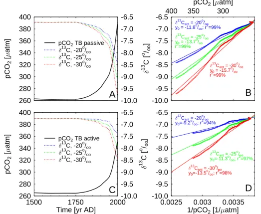
the terrestrial biosphere. In the more realistic case of an active terrestrial biosphere, implying an enhanced photosynthesis and thus carbon uptake through CO₂ fertilisa-tion, pCO₂ at year 2000 is calculated to 351 µatm (Fig.5c). A scenario with passive terrestrial biosphere, meaning a constant carbon storage over time, leads to 388 µatm in the same year (Fig.5a). The annual mean in year 2000 in the atmospheric CO₂data

10

at Point Barrow is 371 ppmv, which is approximately half way between the results of the two different simulation scenarios. The scenario with passive terrestrial biosphere is easier to interprete, since we only have to consider the anthropogenic carbon flux to the atmosphere and the effect of the oceanic sink. Both scenarios will be analysed in the following.

15

The precise value of the δ13C signature of anthropogenic carbon release is still un-certain, e.g. land use change has a δ13C of −25‰ (Scholze et al.,2003), while δ13C of fossil fuel emissions is around −30‰ (Blasing et al.,2004). We therefore varied the isotopic signature of the anthropogenic carbon fluxes between −20‰ and −30‰ to evaluate the importance of this signature for the simulation results. The simulated

20

atmospheric δ13C in year 2000 AD was −8.4, −9.1, −9.7‰ and −7.4, −7.9, −8.4‰ in the scenario with passive and active terrestrial biosphere and for different δ13C sig-natures (−20‰, −25‰, −30‰), respectively (Figs.5a, c), reflecting a larger terrestrial

1

K ¨ohler, P., Muscheler, R., and Fischer, H.: A model-based interpretation of low fre-quency changes in the carbon cycle during the last 120 kyr and its implications for the

reconstruction of atmospheric ∆14C, Geochemistry, Geophysics, Geosystems, in review,

doi:10.1029/2005GC001228, 2006.

(16)

BGD

Full Screen / Esc

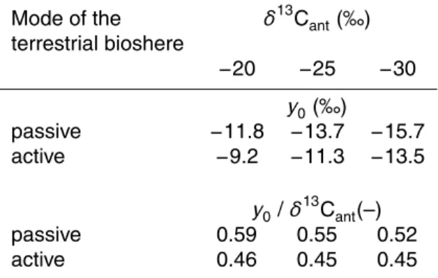
fixation of anthropogenic carbon in the active scenario. The annual average δ13C measured at different globally distributed stations varied between −8.0‰ and −8.2‰ (Keeling et al.,2005).

The regression functions of the Keeling approach are still a good approximation of the artificial data sets (r2≥94%, Figs. 5b, d). However, the y-axis intercept varies

de-5

pending on the assumed δ13C signal of the anthropogenic carbon flux and the mode of the terrestrial biosphere (active/passive) between −9.2‰ and −15.7‰, while the Law Dome data show −13.1‰ (Table 1). Note, that these numbers are significantly higher than the isotopic signature of the anthropogenic carbon added to the system. Due to the non-negligible effect of a third reservoir, the ocean, the Keeling y-axis

inter-10

cept deviates from the expected flux signature derived in Sect.4. Normalised to the

δ13C signal of the anthropogenic flux the y-axis intercept amounts to 52−59% (passive terrestrial biosphere) and 45−46% (active terrestrial biosphere) of the isotopic signal of the anthropogenic flux (Table 1). The difference to an ideal Keeling plot, in which the whole signal would be explained by the y-axis intercept has to be explained purely

15

by oceanic uptake in the case of a passive terrestrial biosphere, and by a mixture of terrestrial and oceanic uptake in simulations with active terrestrial biosphere.

Natural changes in atmospheric CO₂ over the past 650 000 years as recorded in Antarctic ice core records (Petit et al., 1999; Siegenthaler et al., 2005) were always slower and smaller in amplitude than the anthropogenic impact of the last 250 years.

20

Therefore it is conservative to assume that the oceanic uptake of a terrestrial distur-bance in the past will always be greater than during the anthropogenic period. The potential of the Keeling plot approach to paleo climate research therefore seems to have an upper limit. No more than about 50% of the isotopic signature of a carbon source to the atmosphere can be explained with it. In fact, due to the longer time

25

scales on which most processes act during glacial cycles it can be expected that much less than this upper limit can be explained by the Keeling plot approach. For steady state situations (the atmosphere and the ocean are in equilibrium) the perturbation of the carbon cycle through terrestrial carbon release with a signature of −25‰ leads to

(17)

BGD

Full Screen / Esc

a δ_δC→0∆A of about −9‰, as shown in Sect.4. Thus, for this situations only a fraction of 9/25=0.36 is explainable with the Keeling plot approach.

5.3 Glacial/interglacial times

Besides this upper limit of a signal interpretation due to oceanic carbon uptake in long time series two other factors make a comparison of artificial time series with long ice

5

core data sets difficult: First, the air which is enclosed in bubbles in the ice can circulate through the firn down to the depth where bubble close off occurs (∼70−100 m) before it is entrapped in the ice. The bubble close off is a slow process with individual bubbles closing at different times and depth. Accordingly the air enclosed in bubbles and in an ice sample is subject to a wide age distribution acting as an efficient low-pass filter

10

on the atmospheric record. Therefore, all information from the gaseous components of the ice cores is averaged over a time interval of the age of the firn/ice transition zone. This time interval is depending on temperature and accumulation rates, but can roughly be estimated by the ratio of the depth of the firn/ice transition zone divided by the accumulation rate (Schwander and Stauffer,1984). Thus, the time integral in the

15

gas is small (<20 years) at Law Dome (Etheridge et al.,1996), varies at Taylor Dome between 150 years in the Holocene and 300 years in the LGM (Steig et al.,1998a,b), and at EPICA Dome C, at which the most recent CO₂and δ13C measurements were performed (Monnin et al.,2001;Eyer,2004;Eyer et al.,2004;Siegenthaler et al.,2005), between 300 and 600 years (Schwander et al., 2001). Second, the CO₂ and δ13C

20

records retrieved from ice cores are never continuous records, but consist of single measurements with large, but un-regular data gaps in between. In the Taylor Dome ice core these gaps are on average approximately 1000 years wide. It will be therefore of interest to investigate if the temporal resolution in the data set will be sufficient enough to resolve information potentially retrievable through the Keeling approach.

25

Anthropogenic activities add carbon via land use change and fossil fuel emis-sions to the atmosphere, and are only subsequently absorbed by the ocean. The

(18)

BGD

Full Screen / Esc

causes for natural changes in atmospheric CO₂ and thus the carbon cycle during glacial/interglacial times were to a large extent located in the ocean. Thus, the causes and effects respectively their timing are in principle different. For the natural glacial/interglacial variations the carbon content of the atmosphere is determined by the surface ocean, the atmosphere is also called “slave to the ocean”, while for the

5

anthropogenic impact the opposite is the case: The carbon of the surface ocean is modified by the injection of the anthropogenic rise in atmospheric CO₂.

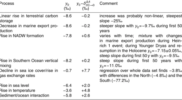
This situation has also consequences for the investigation of different processes causing natural changes in the carbon cycle. We concentrate in the following on the in-dividual impacts of six important processes. We first investigate the maximum impacts

10

possible from changes in these processes and then analyse variations of realistic am-plitude. These processes are changes in terrestrial carbon storage, export production of the marine biota, ocean circulation, gas exchange rates and their variation through variable sea ice cover, and physical effects of variable sea level and ocean temperature. Please note, that in these factorial scenarios all processes can be treated un-coupled

15

in our box model, e.g. changes in the circulation scheme will not lead to temperature variations, which might be the case in general circulation models. A summary of this single process analysis is compiled in Table3. We end with a combined scenario pro-posed byK ¨ohler et al. (2005a) which is able the reconstruct the atmospheric carbon records between 20 and 10 kyr BP. Note, that from these different scenarios only the

20

first one (changes in terrestrial carbon storage) strictly resembles the initial idea of a Keeling plot (addition/subtraction of carbon from the atmosphere).

5.3.1 Terrestrial biosphere

There are two opposing changes in terrestrial carbon storage to be investigated: carbon uptake or carbon release. Both might happen very fast in the course of abrupt

25

climate anomalies, such as so-called Dansgaard/Oeschger events (Dansgaard et al., 1982;Johnsen et al.,1992), during which Greenland temperatures rose and dropped by more than 15 K in a few decades during the last glacial cycle (Lang et al.,1999;

(19)

BGD

Full Screen / Esc

Landais et al.,2004). Terrestrial carbon storage anomalies during these events were estimated with a dynamic global vegetation model to be of the order of 50−100 PgC (K ¨ohler et al.,2005b). The time scales of these anomalies are of the order of centuries to millenia. We first analyse a scenario in which 10 PgC are released or taken up by the terrestrial pools within one year. This short time frame of one year was chosen

5

to have experiments, in which the whole carbon flux is first altering the atmospheric reservoir, before oceanic uptake or release responds after year one. The amplitude of the perturbations is optimised to 10 PgC to guarantee still negligible numerical un-certainties (<0.01‰) in the calculation of the δ13C fluxes. We follow with experiments of linear carbon release and three scenarios of carbon uptake during Termination I to

10

investigate the importance of the time scale for the Keeling plot interpretation.

Fast terrestrial carbon release

This would be the scenario closest to the original Keeling plot analysis in

terres-15

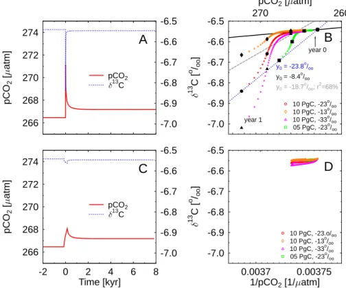
trial ecosystem research. There is a source (terrestrial biosphere) which emits CO₂ directly to the atmosphere. In this experiment, the 10 PgC release first increases

pCO₂ by more than 4 µatm immediately after the release, and equilibrates to less than 1 µatm higher than initially (Fig. 6a). The δ13C signal shows a drop by more than 0.3‰ in year one, and a steady state which is nearly similar to the initial situation

20

(Fig.6a). Near steady state (±0.1%) in both pCO₂ and δ13C was reached 376 years after the carbon release.

There are several possibilities to draw a regression function through the Keeling plot (Fig.6b):

1. A line connecting only the data prior to the start of the carbon release experiment

25

(year 0) and one year later after 10 PgC are released but before any carbon is taken up by the ocean representing the maximum possible slope. Thus, pCO₂ and δ13C after the release can also be calculated following the mass balance equations of a two reservoir system (Eqs.3and4).

(20)

BGD

Full Screen / Esc

2. A straight line through two points characterising the states prior to the carbon release and after re-equilibration. This would contain the minimum information retrievable in case of low sampling frequency and would be the analog to the theoretical considerations for a three reservoir system.

3. A regression function through the subset of points covering the equilibration

pro-5

cess, in which the main dynamics of the carbon release are represented. We here choose all points after the release (year 1) until both pCO₂and δ13C were within ±0.1% of their final steady state values.

It is also of interest if and how the amplitude of the carbon release and its isotopic sig-nature influence the Keeling approach. We therefore performed additional simulations

10

(Figs. 6b, d) with smaller amplitude (5 PgC) and different δ13C signature (−13.5‰, −23.4‰, −33.4‰). These signatures are the result of the variation of the assumed global terrestrial fractionation factor ε_TB=−17‰ by ±10‰.

If such an event of terrestrial carbon release is to be detected in ice cores, we have to manipulate our artificial data set to account for both the temporal integral during gas

15

enclosures and the limited sampling frequency. We assumed an average mixing time (running average of 300 years), and a regular sampling frequency of 100 years, typical for Antarctic ice core studies.

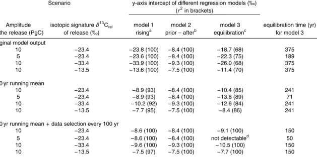
A summary of calculated y-axis intercepts is found in Table2. In the original model output, the regression model 1 (analysis of the carbon flux in the year of the release)

20

can explain the δ13C signature of terrestrial release very well, independent of ampli-tude or the δ13C signature itself. The slight overestimation of the regression model of up to 0.5‰ might be due to numerical limitations. Differences in the y-axis intercept be-tween scenarios with varying amplitude and δ13C signature of the released carbon are still large in regression model 3 (y₀from −18.7‰ to −26.0‰), but a simple functional

25

relationship between y-axis intercept y₀and the δ13C_relsignature of the flux is missing. In model 2 the different δ13C signatures of the carbon release flux are still distinguish-able by small differences in the y-axis intercept (y₀=−7.5‰, −8.4‰, −9.3‰). These

(21)

BGD

Full Screen / Esc

Printer-friendly Version Interactive Discussion y₀’s gained from model 2 are similar to the boundary δ_δC→0∆A introduced in Sect. 4,

which is an embedded feature of the system configuration. Interestingly, the y₀values derived from the BICYCLE simulations are about 1‰ isotopically heavier than in our equilibrium model in Sect.4. The reason for this is the establishing of vertical gradients in DIC and δ13C in the ocean due to the ocean carbon pumps (Volk and Hoffert,1985)

5

leading to an enrichment of δ13C in the surface water by about 1‰.

If we take the signal broadening through temporal mixing in the firn into account (Fig.6bottom), the perturbations in pCO₂ and δ13C are largely reduced to 34% and 7% of their original amplitudes, respectively, and the duration of the atmospheric pCO₂ rise of one year in the original data is now spread over the time length of the smoothing

10

filter (300 yr). Even for conditions similar to those found at Law Dome where the air is mixed only over a time interval of 20 years, the amplitudes in pCO₂ and δ13C are reduced to 70% and 47% of their original values, respectively. Y-axis intercepts for the 300 years smoothing filter are reduced significantly for regression models 1 (30% to 57% of y₀in original data) and 3 (48% to 74% of y₀in original data).

15

A further increase of uncertainty arises if we reduce the sampling interval. The effect of a 100 year sampling frequency reduces y-axis intercepts calculated with regres-sion model 1 and 3 further (Table2). However, the uncertainty introduced by reduced sampling frequency is much smaller than the one based on firn air mixing. Results obtained with regression model 2 (boundary δ_δC→0∆A ) were not affected by any of the

20

two post simulation procedures.

From these fast carbon release experiments, several conclusions can be drawn: 1. The results of regression model 1 are in line with the mass balance equations of

the two reservoir Keeling approach.

2. In all multi-annual experiments the oceanic uptake of carbon will play an important

25

role.

3. Fast terrestrial carbon release events are in their full extent not recordable in the ice core records due to the time integral introduced by the firn enclosure process.

(22)

BGD

Full Screen / Esc

Printer-friendly Version Interactive Discussion Slow terrestrial carbon exchange

To understand glacial/interglacial dynamics one has to investigate larger varia-tions in terrestrial carbon storage of several hundreds of PgC, which occurred over longer time intervals. We have therefore performed additional experiments, one in

5

which 500 PgC is released by the terrestrial pools, but now with a constant release rate over a period of 6000 years. In a second set of experiments we mimic in a simplistic way the carbon uptake of approximately 400 PgC over 6000 yr which might have occurred during the last glacial/interglacial transition between 18 and 12 kyr BP as assumed in three different scenarios (TB0, TB1, TB2) in K ¨ohler et al. (2005a).

10

These scenarios differ in functional dependencies of the terrestrial carbon storage on CO₂fertilisation and climate change (TB0: linear rise in terrestrial carbon; TB1: mainly CO₂ dependent; TB2: mainly climate dependent; Fig.7).

In both linear experiments (carbon release and TB0) the atmospheric δ13C record shows a relaxation behaviour in the first several hundred years after the beginning

15

and after the end of the carbon release with a gradual change in between (Fig. 8). Atmospheric pCO₂ is changing rather constantly over time, also with small nonlinear responses in the first few hundred years at the beginning and at the end of the exper-iment. These discontinuities are caused by the time-delayed oceanic carbon uptake. For example, after the end of the experiment (t=6 kyr, Fig. 8a) large parts of the

re-20

leased carbon are taken up by the ocean in the following centuries, similar as in the fast carbon release experiment shown in Fig.6. In the more complex scenarios TB1 and TB2 the changes in pCO₂ and δ13C are largest in the climate dominated sce-narios TB2 with changing rates of up to 30 µatm in pCO₂ and 0.3‰ in δ13C in 1000 years. In the Keeling plots the relaxation behaviour at the beginning and the end of

25

the linear experiments leads to offsets from the well defined linear relationship. A re-gression over the whole time period leads to a y₀=−8.6‰, only 0.2‰ smaller than the

δ_δC→0∆A boundary for this system. The scatter of the data points is larger in TB1 and TB2 than in the linear experiments, but the regression model through the data is still

(23)

BGD

Full Screen / Esc

very good (r2≥94%) leading to y0=−9.1‰ and −9.0‰, respectively. The slope of the regression is steeper here, because the fractionation factor of the terrestrial biosphere

ε_TB is changing over time. The fraction of terrestrial carbon produced by C₄ photosyn-thesis is decreasing from ∼30% during the LGM to ∼20% during preindustrial times in the scenarios TB1 and TB2 (K ¨ohler and Fischer,2004). This leads to a terrestrial

5

fractionation which is more than 1‰ more negative in the preindustrial times than in the LGM.

The range of the δ13C values concluded from our simulation results for a slow ter-restrial carbon release agrees well with the ones proposed by our theoretical three reservoir approach in Sect. 4 and is very different from the original δ13C of the

car-10

bon source. It is especially remarkable that the differences of the y₀’s from δ_δC→0∆A are very small. Furthermore, these slow carbon exchange processes are so slow that the air enclosure procedure with the assumed smoothing filter of 300 years would only marginally alter the records and would not change the y₀values. Similarly the restricted sampling frequency is of no importance here. These two processes will therefore not

15

be analysed any further in the following, because it is reasonable to assume that their impact on the observed processes can be neglected.

5.3.2 Marine biosphere

While the marine biosphere is in principle a reservoir separate from DIC in the ocean and the atmospheric carbon, it is not independent because the marine export

produc-20

tion establishes vertical gradients in DIC and δ13C between the surface and the deep ocean. Accordingly, the following discussion of changes caused by the marine bio-sphere and other factors represents already a misuse of the Keeling plot approach. Nevertheless it is instructive to study whether the end member analysis can lead to meaningful results and is able to distinguish between different processes.

25

For the marine biota we again first want to explore the range of possible results be-fore we analyse one scenario which seems to be realistic for the last glacial/interglacial

(24)

BGD

Full Screen / Esc

transition. We therefore concentrate first on a switch from an abiotic ocean without any marine biological productivity and no export production to a biotic ocean in year 0 and vice versa. After these biotic/abiotic experiments, the possible effect of an extended glacial marine productivity due to the iron fertilisation in the Southern Ocean is ex-plored. In the biotic ocean a flux of 10 PgC yr−1of organic carbon is exported at 100 m

5

water depth to the deeper ocean. This organic export production is coupled via the rain ratio to an export of 1 PgC yr−1of inorganic CaCO₃.

The abiotic/biotic switch leads to a decrease in atmospheric pCO₂of about 220 µatm and a rise in atmospheric δ13C of 1.0‰ (Fig.9a) and the opposite signals in the bi-otic/abiotic experiment (not shown). The iron fertilisation experiment decreases glacial

10

pCO₂ by 20 µatm, in parallel with a 0.15‰ rise in δ13C (Fig.10a). Here, both atmo-spheric records are relaxing to their preindustrial values after the onset of iron limitation around 18 kyr BP. The Keeling plot analysis leads to y-axis intercepts of −8.0 to −10.2‰ for the three different regression models in the abiotic/biotic experiment (Fig.9b). Com-paring only the prior/after model for all three experiments (abiotic/biotic, biotic/abiotic,

15

iron fertilisation) (Figs.9b, 10b) gives nearly identical results (y₀=−8.7±0.1‰). If the time window of analysis is reduced to the first 50 years after the beginning of the re-duction in export prore-duction in the iron fertilisation experiment a steeper slope in the Keeling plot leads to y₀of −9.7‰ (Fig.10b).

The marine export production combines two of the three ocean carbon pumps: the

20

organic or soft-tissue pump and the carbonate pump (Volk and Hoffert, 1985). The third one, the solubility pump, operates by the increased solubility of CO₂ in down-welling cold water. They all introduce vertical gradients in DIC in the water column, the biological pumps additionally build up a gradient in δ13C. DIC is reduced in the surface layers through marine production of both organic material (soft-tissues) and

25

CaCO₃ and increased in the abyss through carbon released during remineralisation and dissolution. During photosynthesis δ13C is depleted by about −20‰, thus leaving carbon enriched in13C at the surface, while the exported organic matter is depleted. The isotopic fractionation during the production of hard shells slightly enriches13C in

(25)

BGD

Full Screen / Esc

the carbonate (ε ∈[0‰,3‰]). The vertical gradient in δ13C leads to a difference of about 1.0‰ between surface (1.5‰) and abyss (0.5‰) in the biotic ocean, while the

δ13C signal in the abiotic ocean does not change with depth and is around 0.55‰. If we now switch on the marine production in a formerly abiotic ocean we merely introduce these gradients to the system. Surface δ13C is rising by 1.0‰ and so is the

atmo-5

spheric δ13C. The signal seen in the atmospheric record is therefore a mixture of the fractionation during gas exchange and an increased carbon flux from the atmosphere to the ocean. In BICYCLE the flux of CO₂ from the surface ocean to the atmosphere has a fractionation factor of ε_O2A≈−10.4‰ and ε_A2O≈−2.4‰ in the opposite direction leading to a net fractionation effect of −8.0‰ (but both depend also on temperature,

10

and ε_O2A additionally on DIC, HCO−₃, and CO2−₃ ). Similar as in the previous case of a terrestrial carbon release the system contains a boundary in the effective isotopic signature. Each perturbation of the system leads to a derivation from this boundary. The effects of changes in the marine carbon fluxes on atmospheric pCO₂ and δ13C are not necessary the same as for the terrestrial case. Therefore, the boundary is not

15

identical with δ_δC→0∆A , but seems to be very close. From variations of the global export production one can estimate this marine boundary to be around −8.5‰. In year 1, for example, one can understand the signal (y₀=−10.2‰) in the following way: In areas in which marine export production is reducing surface DIC the gross carbon flux from the ocean to the atmosphere is largely reduced. In the most extreme case we would

20

only find a gross carbon flux from the atmosphere to the ocean with the corresponding fractionation factor ε_A2O=−2.4‰. This would be the isotopic signature of the process in action and added to the marine boundary it would lead at maximum to a y₀of −10.9‰. The calculated y₀is smaller because there is still a small but not negligible gross flux of CO₂from the ocean to the atmosphere. The signal during the first 50 years of the iron

25

fertilisation experiment (y₀=−9.7‰) can be interpreted similarly. During the latter part of the abiotic/biotic switch experiment and over the equilibration period y₀ is ∼−8.0‰ and thus more positive than the marine boundary. This might be caused by the in-creased δ13C of the DIC in the surface waters. After 100 years, pCO₂ has already

(26)

BGD

Full Screen / Esc

dropped to 346 µatm, thus nearly 2/3 of the oceanic uptake of carbon happens in this first century. Therefore the carbon fluxes from the atmosphere to the ocean and vice versa are nearly similar thereafter. That means that now the isotopic enriched DIC of the surface waters can enter the atmosphere and is then enriching δ13C and y₀.

If compared with the terrestrial experiments the results from regression model 3

5

(prior/after analysis) have y₀’s which are only 0.2 to 0.4‰ more negative than δ_δC→0∆A . This is very similar to the experiments with slow carbon exchange between the terres-trial biosphere and the atmosphere.

5.3.3 Ocean circulation

PreviouslyK ¨ohler et al. (2005a) assumed a rise in the strength of the North Atlantic

10

Deep Water (NADW) formation from 10 Sv (106m3s−1) during the Last Glacial Max-imum (LGM) to intermediate levels of 13 Sv in the Bølling/Allerød warm interval and 16 Sv at the beginning of the Holocene. This rise was punctuated by sharp drops in the NADW formation strength and the subsequent ocean circulation fluxes to 0 Sv and 11 Sv during the Heinrich 1 event and the Younger Dryas, respectively. Repeating this

15

temporal sequence of events over a period of approximately 6000 years leads to drops in pCO₂by 10 µatm during times of reduced ocean circulation accompanied by rises in δ13C of about 0.05‰. Initial and final values differ by about 15 µatm and −0.05‰ (Fig.11a).

The prior/after analysis in the Keeling plot leads to a y-axis intercept of −7.8‰,

how-20

ever, the pattern is highly time-dependent and allows a breakdown of the time series into the individual events, which show distinctively different behaviour. These events are marked in Figs.11a, b (1: decrease in NADW formation during Heinrich 1 event; 2: increase in NADW formation during Bølling/Allerød warm interval; 3: decrease in NADW formation during Younger Dryas; 4: increase in NADW formation towards

inter-25

glacial levels). The regression analysis over the whole of these four periods, which last between 1200 and 2000 years each, finds y-axis intercepts between −5.3 and −7.2‰.

(27)

BGD

Full Screen / Esc

If shorter time windows after the beginning of these changes in ocean circulation are analysed, much steeper regression functions can be found. For example, the regres-sions through 50 year time windows at the beginning of interval 2 and 4, which show the steepest slopes in the Keeling plot, lead to y-axis intercepts of −39.1 and −9.5‰, respectively (Fig.11b).

5

The complete shut-down of the NADW formation during Heinrich 1 event alters also the nutrient availability for the marine biota. The export of organic matter depends on the availability of macro-nutrients in the surface waters and is prescribed to an upper limit of 10 PgC yr−1. In the time interval between 16.5 and 15 kyr BP marine export falls from 10 PgC yr−1 to 8.9−9.3 PgC yr−1. Less export production increases atmospheric

10

pCO₂and decreases atmospheric δ13C. This implies that the peaks in the atmospheric carbon records were both dampened during interval 1. Accordingly, the y₀derived from the Keeling plot during this time interval is a mixture of ocean circulation and marine biota.

A second ocean circulation process which changed according toK ¨ohler et al.(2005a)

15

over the time of the last transition was the Southern Ocean vertical mixing rate (Figs.11c, d). It rose from 9 Sv (glacial) to 29 Sv (preindustrial) and led to a rise in

pCO₂ by about 30 µatm and a drop in δ13C by more than 0.2‰. Here, the Keeling plot interpretation gives us a y-axis intercept of −8.2‰ for the prior/after analysis. The steepest slope during the first 50 years after the start of the change would yield to a

20

y-axis intercept of −11.0‰ (Fig.11d).

The overturning circulation distributes carbon in the ocean. Its effect on the at-mospheric carbon reservoirs, however, is opposite to that of the three ocean carbon pumps. While the pumps introduce vertical gradients in DIC and δ13C as described in the subsection about the marine biota, the overturning circulation is reducing these

25

vertical gradients again through the ventilation of the deep ocean which brings water rich in DIC and depleted in13C back to the surface. A weakening of the ventilation reduces these upwelling processes and leads to lower pCO₂and higher δ13C values as seen in the experiments.

(28)

BGD

Full Screen / Esc

The y₀-values derived from the four intervals for changing NADW formation differ. Between interval 3 and 4 in which opposing changes in ocean circulation occur, the differences in the y₀-values are small. These different circulation patterns can be seen in the Keeling plot in the dynamics of the first years of the intervals: In intervals 1 and 3, in which the strength of the NADW formation is reduced, the analysis of a time window

5

at the beginning of the interval leads to less negative y₀ than over the whole period, while the opposite is the case in the intervals 2 and 4 with a resumption of the NADW formation. These temporal changes over the course of each interval are caused by the equilibration of the model to a new steady state. In interval 1, the shutdown of the NADW and the subsequent fluxes lead first to an enrichment of DIC and of13C in

10

the North Atlantic surface waters and thus to higher atmospheric δ13C. Later-on, this is over-compensated by decreasing DIC and δ13C in the equatorial surface of the Atlantic Ocean. However, the dynamics during a complete shutdown of the NADW formation might be unrealistic because in the current model configuration the tropical Atlantic surface and intermediate ocean boxes would exchange water with each other but not

15

with any other water masses (Fig.4). This artefact is also responsible for the dynamics during the first years of interval 2, but is not affecting the latter intervals.

Compared to the terrestrial carbon release we can say that a change in ocean cir-culation is assigned to a y₀slightly more positive than the terrestrial boundary δ_δC→0∆A (+0.2 to +1.2‰). The dynamics during the first years of a abrupt rise/decrease in the

20

strength of the overturning circulation lead to larger offsets (fall/rise) from the terrestrial boundary.

5.3.4 Gas exchange/sea ice

A change in sea ice cover leads to changes in the gas exchange rates with opposing effects for the northern and the southern high latitudes. As the preindustrial North

25

Atlantic Ocean is a sink for CO₂ a reduced gas-exchange due to higher sea ice cover leads to rising atmospheric pCO₂, while the same happening in the Southern Ocean being a source for CO₂leads to a drop in pCO₂. Again, we first explore the maximum