HAL Id: hal-03022874
https://hal.archives-ouvertes.fr/hal-03022874
Submitted on 25 Nov 2020
HAL is a multi-disciplinary open access
archive for the deposit and dissemination of
sci-entific research documents, whether they are
pub-lished or not. The documents may come from
teaching and research institutions in France or
abroad, or from public or private research centers.
L’archive ouverte pluridisciplinaire HAL, est
destinée au dépôt et à la diffusion de documents
scientifiques de niveau recherche, publiés ou non,
émanant des établissements d’enseignement et de
recherche français ou étrangers, des laboratoires
publics ou privés.
Kalkayotl: A cluster distance inference code
J. Olivares, L. M. Sarro, H. Bouy, N. Miret-Roig, L. Casamiquela, P. A. B.
Galli, A. Berihuete, Y. Tarricq
To cite this version:
J. Olivares, L. M. Sarro, H. Bouy, N. Miret-Roig, L. Casamiquela, et al.. Kalkayotl: A cluster distance
inference code. Astronomy and Astrophysics - A&A, EDP Sciences, 2020, 644, pp.A7.
�10.1051/0004-6361/202037846�. �hal-03022874�
https://doi.org/10.1051/0004-6361/202037846 c J. Olivares et al. 2020
Astronomy
&
Astrophysics
Kalkayotl: A cluster distance inference code
J. Olivares
1, L. M. Sarro
2, H. Bouy
1, N. Miret-Roig
1, L. Casamiquela
1, P. A. B. Galli
1, A. Berihuete
3, and Y. Tarricq
11 Laboratoire d’astrophysique de Bordeaux, Univ. Bordeaux, CNRS, B18N, allée Geoffroy Saint-Hilaire, 33615 Pessac, France e-mail: javier.olivares-romero@u-bordeaux.fr
2 Depto. de Inteligencia Artificial, UNED, Juan del Rosal, 16, 28040 Madrid, Spain
3 Depto. de Estadística e Investigación Operativa , Universidad de Cádiz, Campus Universitario Río San Pedro s/n, 11510 Puerto Real, Cádiz, Spain
Received 28 February 2020/ Accepted 26 September 2020
ABSTRACT
Context.The high-precision parallax data of the Gaia mission allows for significant improvements in the distance determination to stellar clusters and their stars. In order to obtain accurate and precise distance determinations, systematics such as parallax spatial correlations need to be accounted for, especially with regard to stars in small sky regions.
Aims.Our aim is to provide the astrophysical community with a free and open code designed to simultaneously infer cluster param-eters (i.e., distance and size) and distances to the cluster stars using Gaia parallax measurements. The code includes cluster-oriented prior families and it is specifically designed to deal with the Gaia parallax spatial correlations.
Methods.A Bayesian hierarchical model is created to allow for the inference of both the cluster parameters and distances to its stars.
Results.Using synthetic data that mimics Gaia parallax uncertainties and spatial correlations, we observe that our cluster-oriented prior families result in distance estimates with smaller errors than those obtained with an exponentially decreasing space density prior. In addition, the treatment of the parallax spatial correlations minimizes errors in the estimated cluster size and stellar distances, and avoids the underestimation of uncertainties. Although neglecting the parallax spatial correlations has no impact on the accuracy of cluster distance determinations, it underestimates the uncertainties and may result in measurements that are incompatible with the true value (i.e., falling beyond the 2σ uncertainties).
Conclusions.The combination of prior knowledge with the treatment of Gaia parallax spatial correlations produces accurate (error <10%) and trustworthy estimates (i.e., true values contained within the 2σ uncertainties) of cluster distances for clusters up to ∼5 kpc, along with cluster sizes for clusters up to ∼1 kpc.
Key words. methods: statistical – parallaxes – open clusters and associations: general – stars: distances – virtual observatory tools
1. Introduction
Stellar clusters offer a unique opportunity to test models of the formation and evolution of stars and stellar systems. Their distance is useful for the comparison of model predictions to observations when the observational uncertainties are taken into account. Traditionally, these comparisons use the cluster dis-tance, which is typically more precise than the distances of indi-vidual stars. However, high-precision astrometric surveys, such
as H
ipparcos
(ESA 1997;Perryman et al. 1997) and Gaia (GaiaCollaboration 2016, 2018), have pushed these comparisons at the level of individual stars, at least for the most precise mea-surements of the nearest systems. Therefore, while determin-ing cluster distances remains a fundamental problem, retrievdetermin-ing the distances to the cluster stars allows astronomers to perform detailed tests of current theories of star formation and evolution; see, for example, the analyses of internal dynamics and 3D struc-tures done byWright & Mamajek(2018),Galli et al.(2019), and
Armstrong et al.(2020).
Since the cluster distance is an important parameter, diverse methodologies have been developed to estimate it either from photometry, astrometry, or combinations of both (e.g., Palmer et al. 2014;Perren et al. 2015;Gaia Collaboration 2017;Galli et al. 2017;Yen et al. 2018). In the context of distance determi-nation based on parallax measurements, the traditional approach consists of averaging the parallaxes of the cluster stars and
then inverting the resulting (more precise) parallax mean. More sophisticated approaches have also been devised. For example,
Palmer et al.(2014) developed a maximum-likelihood approach for open cluster distance determination. In their study, the authors assumed that the spatial distribution of stars in open clus-ters follows a spherical Gaussian distribution and they inferred the cluster distance together with its dispersion and other kine-matic parameters by marginalizing the positions of individual stars. They validated their methodology on synthetic clusters with properties similar to those expected for the Gaia data. Then,Gaia Collaboration(2017) determined astrometric param-eters of open clusters by modeling their intrinsic kinematics and projecting them in the observational space.Cantat-Gaudin et al.(2018) obtained open-cluster distances using a maximum-likelihood method. Nonetheless, they neglect the cluster intrinsic depth, which results in underestimated distance uncertainties.
Although they were devised outside the context of open clus-ters, the following Bayesian frameworks are worthy of mention due to their use of Gaia parallax measurements and specific prior information. Bailer-Jones et al.(2018) inferred posterior distance distributions to 1.3 billion stars in the Gaia data using a Galactic weak distance prior specifically designed for the entire Galaxy.Anders et al.(2019) obtained distances to stars brighter than G= 18 mag using a Galactic multi-component prior (with halo, bulge, and thin and thick disks), and a combination of Gaia measurements (including parallax) and photometry from several
Open Access article,published by EDP Sciences, under the terms of the Creative Commons Attribution License (https://creativecommons.org/licenses/by/4.0),
surveys.Wright & Mamajek(2018) developed a forward-model for the inference of parameters of OB associations. Their model uses a 3DElson et al.(1987) profile that includes the distance to the association as a free parameter. However, they inferred the individual stellar distances using the Galactic distance prior proposed by Bailer-Jones et al.(2018). In addition, the online resources1recommended byLuri et al.(2018) provide detailed steps for the inference of cluster distance and size. Recently,
Perren et al.(2020) used the insight provided by these online resources to infer cluster distances based on a Gaussian prior. These authors marginalize the individual distances as well as the cluster intrinsic dispersion.
The previous studies can be classified into those that infer population parameters of either clusters and associations by mar-ginalizing individual stellar distances (e.g.,Wright & Mamajek 2018; Perren et al. 2020, and the online resources mentioned above) and those that infer individual stellar distances but do not infer the population parameters (e.g.,Bailer-Jones et al. 2018;
Anders et al. 2019). To the best of our knowledge, the simultane-ous inference of population parameters and individual distances has not been addressed in the literature. Furthermore, none of the aforementioned methodologies is able to deal with the systemat-ics introduced by the parallax spatial correlations present in the Gaiadata (see Sect. 5.4 ofLindegren et al. 2018).
Following the guidelines provided byLuri et al. (2018), in this work, we attempt to solve the aforementioned issues in the specific context of stellar clusters by providing the astrophysi-cal community with the free open code Kalkayotl2. It samples the joint posterior distribution of the cluster parameters and stel-lar distances, based on their Gaia astrometric data and a set of cluster-oriented prior families.
Our approach is different from that adopted in the afore-mentioned works. While Bailer-Jones et al. (2018),Wright & Mamajek(2018), andAnders et al.(2019) analytically or numer-ically find statistics of the stars posterior distance distributions using a unique Galactic prior, Kalkayotl obtains samples of the posterior distribution of the star and cluster parameters for a set of cluster oriented prior families by means of Hamiltonian Monte Carlo (Duane et al. 1987), which is a type of Markov chain Monte Carlo (MCMC) technique. This approach offers the user the advantage of taking an active criticism over the prior (i.e., choose its family, infer its parameters, and compare with results from other prior families), together with an easier prop-agation of uncertainty into subsequent analyses. On the other hand, the MCMC approach has the constraint of being compu-tationally expensive. In a machine with four CPUs at 2.7 GHz, Kalkayotltakes typically five minutes to run the inference model of a cluster with one thousand stars, although the running time can increase depending on the prior complexity and quality of the data set.
The rest of this work is organized as follows. In Sect.2, we introduce the methodology of Kalkayotl. In Sect.3, we construct synthetic clusters that mimic the Gaia data and in Sect.4, we use these clusters to validate the methodology. Finally, in Sect. 5, we discuss the advantages and caveats of our methodological approach and present our conclusions.
1
https://github.com/agabrown/astrometry-inference-tutorials, and
https://github.com/ehalley/parallax-tutorial-2018
2 Kalkayotl means distance in the mesoamerican Nahuatl language.
2. Methodology
Kalkayotl is a free python code3 designed to simultaneously sample the joint posterior distribution of cluster parameters and stellar distances. In addition, the user can decide to only sam-ple the stellar distances by fixing the cluster parameters and to perform the sampling on the parallax space (i.e., sampling the clusters’ and sources’ true parallaxes). The latter can be useful when the subsequent analyses need to be done on the parallax space. Although the methodology can be applied to any parallax measurement, Kalkayotl is specifically designed to work with Gaiaastrometric data. Users will also be able to run the code through the Spanish Virtual Observatory, however, with certain limitations.
2.1. Assumptions
Prior to a presentation of the details of the methodology, we state the assumptions we made at the start.
Assumption 1. The Gaia astrometric measurements are nor-mally distributed around the true values. As explained in Sect. 5.2 ofLindegren et al.(2018), the standardized astrometric measurements are almost4 normal. The Gaia catalog provides all necessary information (i.e., mean, standard deviations, and correlations) to reconstruct these distributions.
Assumption 2. The Gaia parallax measurements are shifted from their true values and this shift can be different for differ-ent sky positions, colors, and magnitudes (Gaia Collaboration 2018). Extensive studies have been carried out to determine this parallax zero point and its correlations with other observables and stellar types (see Fig. 14 ofChan & Bovy 2020, and refer-ences therein). The user can set the parallax zero point value5 and, if desired, use different values for different sources.
Assumption 3. The Gaia astrometric measurements of dif-ferent sources are spatially correlated among them. We use the covariance functions proposed byVasiliev(2019), which provide a better description to the observed correlations at small angular separations than those ofLindegren et al.(2018); compare Fig. 2 of the former author to Fig. 15 of the latter authors. The parallax covariance function ofVasiliev(2019) is given by:
V(θ)= 0.0003 · exp(−θ/20◦) + 0.002 · sinc(0.25◦+ θ/0.5◦
) mas2, (1)
where θ is the angular separation between two sources.
Assumption 4. The cluster size is much smaller than its dis-tance. If the cluster size is comparable to its distance, then using only the line of sight distances results in biased estimates of the cluster distance due to projection effects.
Assumption 5. The input list of cluster members is neither contaminated nor biased (i.e., we assume a perfect selection function).
As in any Bayesian methodology, we then proceed to specify the likelihood, prior, and the procedure for obtaining the poste-rior distribution.
3 The code and documentation is available at: https://github.
com/olivares-j/Kalkayotl
4 The standard deviations of the standardized parallax, and proper motions in RA and Dec, are 1.081, 1.093 and 1.115, respectively. Thus the errors are 8–12% larger than the formal uncertainties.
5 The parallax zero point uncertainty can be included by adding it to the parallax uncertainty of the sources.
2.2. Likelihood
The likelihood of the N observed sources with data D = {$i, σ$,i}iN=1(where $iand σ$,iare the mean and standard
devi-ation that define the parallax measurement of source i), given the Θ parameters can be represented as
L(D|Θ) ≡ L({$i}Ni=1|T (Θ), {σ$,i} N
i=1)= N(X − Xzp|T (Θ), Σ), (2)
where N(·|·) represents the multivariate normal distribution (see Assumption1), X the N-dimensional vector of the observed par-allax, Σ the N × N covariance matrix, Xzp the N vector of zero
points, and T the transformation from the parameter space to the space of observed-quantities.
In the set of parametersΘ = {θi}iN=1, the parameter θiof the
ith source represents its true distance. Therefore, T is equal to 1000/θ, with θ in pc and the result in mas. If the user decides to do so, the sampling can be done in the parallax space, in which case θicorresponds to the source true parallax, and T is the
iden-tity relation. Nonetheless, hereafter, we set our work in the dis-tance space.
The vectors X and Xzp are constructed from the
concatena-tion of the N vectors of observaconcatena-tions {$i}Ni=1 and zero-points
$zp respectively (see Assumption2). The covariance matrix Σ
contains the N-dimensional vector of variances, {σ2
$,i}Ni=1, in its
diagonal, whereas the off-diagonal terms are the covariances between the parallax measurements of different sources (see Assumption3).
2.3. Prior families
The prior distribution is supposed to encode the previous knowl-edge of the investigator about the plausibility of the parame-ter values in a model. In the case of stellar clusparame-ters, we know that their stars share common distributions of their astrophysi-cal properties, like their distance to the observer, age, metallic-ity, etc.. This a priori information is what we use to construct an informed prior. Nonetheless, given the variety of cluster mor-phologies, we believe that there is no universal prior for clusters. In Kalkayotl, we propose two types of distance-prior families, one based on classical statistical probability density distributions and another based on purely astrophysical consid-erations. The purely statistical ones are common distributions used in the literature, while the astrophysical ones are inspired by previous works devoted to the analysis of the luminosity (or number) surface density profiles of galactic and globular clusters. The purely statistical prior families are parametrized only by their location, loc, and scale, scl, which are defined as follows. The location, loc, is the expected value of the cluster distance, while the scale, scl, is the typical scale length of the cluster along the line of sight. Our statistical prior families are the following. The uniform prior family is the simplest one, as it assigns the same probability density to all values in the inter-val [loc − scl, loc+ scl]. The Gaussian prior family assumes that the distance is normally distributed with mean, loc, and stan-dard deviation, scl. The Gaussian mixture model’s prior family (GMM) assumes that the distance distribution is described by a linear combination of k Gaussian distributions, with k an integer greater than zero. In the following, we use k = 2. We also ana-lyzed other types of distributions (such as Cauchy, half-Cauchy, and half-Gaussian) but they returned poorer results when com-pared to the previously mentioned prior families and, thus, we do not include them in our analysis.
The astrophysical prior families are parametrized as well by the location loc and scale scl parameters, but they contain even
more information, as we describe below. The loc parameter still describes the most typical cluster distance, while the scl one now corresponds to what is commonly referred to as the core radius (i.e., the typical size of the cluster inner region). It is important to notice that although the astrophysical distance prior families have similar functional forms to the luminosity (or number) sur-face density profiles which they were were inspired by, there is no correspondence between them; while the latter are defined as surface densities, the former are defined as distance densities.
The Elson, Fall, and Freeman prior family (EFF) distributes the distances in a similar way asElson et al.(1987) distributed the surface luminosity density of clusters from the Large Mag-ellanic Cloud. In addition to the location and scale parameters, it utilizes the γ parameter which describes the slope of the dis-tribution at large radii. In the standardized form (loc = 0 and scl= 1), the EFF is defined as:
EFF(r|γ)= √ Γ(γ) π · Γ(γ − 1
2)
·h1+ r2i−γ, (3) withΓ the gamma function, and r the standardized distance. In our parametrization, γ = γ0/2, with γ0 the original parameter proposed by Elson et al. (1987). We notice that by fixing the γ parameter to 1 or 5/2 the EFF prior family is reduced to the Cauchy and Plummer distributions, respectively.
The King prior family distributes the distances in a similar way asKing (1962) distributed the surface number density of globular clusters. In addition to the location and scale parame-ters, it includes the maximal extension of the cluster through the tidal radius parameter, rt; the probability distribution is thus
nor-malized within this distance. In its standardized form (loc= 0, core radius= scl = 1), the King prior is defined as
King(r|rt)= " 1 √ 1+r2− 1 √ 1+r2 t #2 2 " rt 1+r2 t −2arcsinh(r√ t) 1+r2 t + arctan(rt) # , (4)
with r as the standardized distance.
For completeness, Kalkayotl also includes the Galactic expo-nentially decreasing space density (EDSD) prior6introduced by
Bailer-Jones (2015). We refer to the aforementioned work for an explicit definition of this prior. It suffices to say that its only parameter, scl, is the typical length of exponential decay. In this work, our objective is to estimate distances to stars in clusters, and not in the field population, thus we include it only for com-parison purposes. We are perfectly aware that this constitutes an unfair comparison but we want to emphasize the problems associated with adopting a Galactic prior for the inference of distances in a cluster scenario.
2.4. Hyper-priors
If the user decides to infer the cluster parameters, φ= {loc, scl}, together with the source parametersΘ, then a hierarchical model is created with the cluster parameters at the top of the hierarchy. In this case, a prior must be set for each parameter of the chosen cluster prior family. In the Bayesian jargon, this kind of prior is called hyper-prior, and its parameters are hyper-parameters.
As hyper-prior for the location, loc, and scale, scl, we use the Normal(loc|α) and Gamma(scl|2,2/β) densities respectively, 6 We do not refer to it as a prior family since its only parameter, the scale length, will be kept fixed throughout this analysis.
where α and β are their hyper-parameters. The Gamma distri-bution and its hyper-parameters are specified following the rec-ommendations ofChung et al.(2013). The specific choice of the rate parameter as 2/β in the Gamma distribution results in the mean of the latter at β.
The weights, {wi}ki=1in the GMM prior family are Dirichlet
({wi}ki=1|δ) distributed, with δ the k-th vector of hyper-parameters.
The γ parameter in the EFF prior family is distributed as γ ∼ 1 + Gamma(2, 2/γhyp) with γhypprovided by the user; this
parametrization avoids γ < 1, which will produce extreme cluster tails. For the tidal radius in the King prior family, we use a sim-ilar weakly informative prior: rt ∼ 1+ Gamma(2, 2/γhyp) with
γhypan hyper-parameter provided by the user. We notice that the
tidal radius is in units of the core radius (i.e., scale parameter) and, thus, it is restricted to be larger than one.
2.5. Posterior distribution
Bayes’ theorem states that the posterior distribution equals the prior times the likelihood normalized by the evidence Z. If the user of Kalkayotl decides to infer only the distances to the indi-vidual sources, this is only theΘ parameters, then the posterior distribution is given by
P(Θ | D) = L(D |Θ) · π(Θ | φ)
Z , (5)
where the likelihood L is given by Eq. (2). The prior π is one of the prior families described in Sect.2.3for which its parameters, φ have been fixed to a user decided value. Finally, the evidence Z is simply the normalization factor.
On the other hand, if the user decides to infer both the source distances,Θ, and the cluster parameters, φ, then the posterior is given by
P(Θ, φ | D) = L(D |Θ) · π(Θ | φ) · ψ(φ)
Z , (6)
where now ψ is the hyper-prior of the cluster parameters φ. We notice that this latter case should not be used in combination with the EDSD prior because it will be meaningless to infer the scale length of a Galactic prior based on data from the population of a single Galactic cluster.
In Kalkayotl, the posterior distribution is sampled using the Hamiltonian Monte Carlo method implemented in PyMC3 (Salvatier et al. 2016), which is a Python probabilistic program-ming framework. For details of the capabilities and caveats of Hamiltonian Monte Carlo samplers on hierarchical models we refer the reader to the work of Betancourt & Girolami(2013). In particular, our model faces the typical problems of sampling efficiency associated with hierarchical models. Thus, following the recommendations of the aforementioned authors, Kalkayotl allows the user to choose between the central and non-central parametrizations (except for the GMM prior family, which con-tains more than one scale parameter). While the non-central parametrization enables more efficient sampling in the presence of data sets with limited information (i.e., few members and large uncertainties), the central one works better for more constraining ones (i.e., nearby and well-populated clusters).
The PyMC3 framework provides different initialization schemes for the MCMC chains, and a set of tools to automati-cally diagnose convergence after sampling. Here, we choose the advi+adapt_diag initialization scheme7, because it proved to 7 The interested reader can find more details about initialization schemes and convergence diagnostics at the PyMC3 documentation:
https://docs.pymc.io/
be the most efficient one for reducing both the number of tun-ing steps (thus the total computtun-ing time) and initialization errors (like those of “bad initial energy” or “zero derivative” for a cer-tain parameter). This method starts the chain at the test value (which depends on the prior but is usually its mean or mode) and runs the automatic differentiation variational inference algo-rithm, which delivers an approximation to the target posterior distribution.
Once the initialization is complete, the code performs the inference in two stages. First, the sampler is tuned, and then the posterior samples are computed. The number of tuning and sampling steps are chosen by the user. While sampling steps are established based on the desired parameters precision8, the number of tuning steps depends on the complexity of the poste-rior. Typical values of the tuning steps are 1000 and 10000 for the simple (i.e., uniform and Gaussian) and complex (i.e., EFF, King, and GMM) prior families, respectively.
Once the inference is done, the convergence of the chains is assessed based on the Gelman-Rubin statistic, effective sam-ple size, and the number of divergences (see Note7). Kalkay-otlthen discards the tuning samples (to avoid biased estimates) and reports cluster and source summary statistics (the desired percentiles and the mode, median, or mean). In addition, it also makes trace plots of the cluster and source parameters. Although the automatic analysis made by PyMC3 usually suffices to ensure convergence, we strongly recommend users to visually inspect the chains to ensure that no anomalies are present.
As in most Bayesian inference problems, the investigator must face the decision of choosing the most suitable prior. The rule of thumb is that there is no universal prior, and the most suitable prior depends on the specific problem at hand. Thus, to help users decide which prior family might be the most suitable for their data sets, Kalkayotl offers a module to make compar-ison of models by means of Bayes factors, which are the ratio of the Bayesian evidence (Z in Eqs. (5) and (6)) of each pair of models. Estimating the Bayesian evidence is a hard and compu-tationally expensive problem, thus, in order to reduce the com-putation time, additional assumptions are needed. The reader can find these additional assumptions together with details of the evi-dence computation in AppendixA. Once the Bayesian evidence of each model is computed, the decision can be taken based on
Jeffreys(1961) scale9.
In summary, Kalkayotl returns samples of the joint poste-rior distribution of the cluster parameter and stellar distances, together with summary statistics thereof. In addition, the user can do model selection based on the Bayes factors. However, we notice that the evidence computation is expensive, taking at least three and ten times more time than the posterior sampling of the purely statistical and astrophysical prior families, respectively.
3. Synthetic clusters
Our aim in this section is to create synthetic clusters with parallax uncertainties and spatial correlations similar to those 8 The parameter precision is given by the standard error of the mean: σ/√n, where σ is the posterior standard deviation, and n its effective sample size (i.e. number of independent samples from the posterior distribution). This last value is reported by the sam-pler and is proportional to the input value of sampling steps given by the user and the sampler efficiency. For details of its computa-tion seehttps://mc-stan.org/docs/2_18/reference-manual/ effective-sample-size-section.html
9 In this scale, the evidence is: inconclusive if the Bayes Factor is <3:1, weak if it is ∼3:1, moderate if it is ∼12:1, and strong if it is >15:1.
present in the Gaia data. These synthetic clusters will then be used to validate our methodology, in particular, its accuracy and precision as a function of cluster distance and the number of sources.
The Gaia parallax uncertainty depends on the source mag-nitude, colour and number of transits (see Gaia Collaboration 2018;Lindegren et al. 2018). Thus, to generate realistic parallax uncertainties we simulate the photometry of our sources with the isochrones python package (Morton 2015). The mass of each source was randomly drawn from a Chabrier mass distribution (Chabrier et al. 2005) and its photometry computed by means of the MIST models (Dotter 2016;Choi et al. 2016). For the latter, we use solar metallicity, zero extinction, and the typical open-cluster age of 158 Myr, which corresponds to the mean age of the 269 open clusters analyzed byBossini et al.(2019). We explore a grid of distances from 100 pc to 1 kpc at steps of 100 pc, and from 1 kpc to 5 kpc at steps of 1 kpc. We use 100, 500, and 1000 sources, these cover the typical numbers of clusters members.
The radial distance of each source to the cluster center was drawn from each of our distance prior families and its 3D Carte-sian coordinates were then computed. We notice that these result in spherically symmetric distributions, which suffices for the purposes of the present analysis.
To account for random fluctuations, we repeat ten times each simulation of our grid (main distance, number of sources, and distance distribution). We use ten parsecs as the typical cluster scale, and for the EFF and King prior we set their γ and stan-dardized tidal radius parameters to 3 and 5, respectively. In the GMM synthetic clusters, we use for the second component a dis-tance 10% larger than the main disdis-tance, and a scale of 20 pc. The fraction of sources in each component was set to 0.5.
Then, we use PyGaia10to obtain parallax uncertainties (from the G, and V-I photometry together with nominal GDR2 time baseline) and to transform the true source coordinates into true sky positions and parallaxes.
Afterwards, we use sky positions, parallax uncertainties, and
Vasiliev (2019) parallax spatial correlation function to com-pute the covariance matrix Σ, which is constructed by adding the covariance matrix of the parallax uncertainties (i.e., a diagonal matrix with parallax variances in the diagonal) plus the covariance matrix of the parallax spatial correlations (see Assumption3). Then, the observed parallaxes were drawn from a multivariate normal distribution centered on the true parallaxes and withΣ as the covariance matrix. We did not include any par-allax zero-point shift in our synthetic data sets. We end up with a total of 2100 synthetic clusters containing 1.12 million sources.
4. Validation
In this section, we measure the accuracy, precision, and credi-bility of our methodology at estimating the true values of both the population and source parameters (further details and addi-tional figures can be found in AppendixB). We measure accu-racy and precision as the fractional error (i.e. the posterior mean minus the true value divided by the true value) and the fractional uncertainty (i.e., the 95% posterior credible interval divided by the true value), respectively. We define credibility as the per-centage of synthetic clusters realizations in which the inferred 95% posterior credible interval contains the true value (i.e., the true value is covered by the 2σ uncertainties). This defini-tion of credibility measures the trustworthiness of the inferred value and its reported uncertainty. In this section, we also
com-10 https://github.com/agabrown/PyGaia
pare the distance estimates delivered by different prior fami-lies when applied to the same synthetic cluster. Furthermore, we analyze the sensitivity of our methodology to the choice of hyper-parameter values, the detail of this analysis can be found in AppendixC. In brief, we find that the results of our methodology are insensitive to changes of up to 10% and 50% in the hyper-parameters of the location and scale parameters, respectively.
Additionally, we use our set of synthetic clusters to explore the accuracy, precision, and credibility of the commonly used approach of inverting the mean parallax of the cluster stars. The results of this analysis are shown in Appendix D. In brief, we observe that this approach returns cluster distance estimates with low fractional errors (<5%) when the cluster is located closer than 1 kpc. However, beyond that limit, the approach is suscepti-ble to large random errors (>10%), as already reported byPalmer et al.(2014). Moreover, the low uncertainties obtained by invert-ing the mean parallax, result in smaller credibilities than those obtained by our methodology over the same data sets (compare Fig.D.1with the left column of Fig.B.2). The only exception being the closest clusters, at 100 pc, where the validity of our Assumption4is the weakest.
4.1. Accuracy and precision
Concerning the population parameters, we find that the clus-ter distance is accurately declus-termined by all our prior families, with a fractional error smaller than 10%. The cluster scale accu-racy depends on the chosen prior family, the number of cluster sources, and the cluster distance. This parameter is accurately determined, with a fractional error smaller than 10%, by the uni-form, Gaussian, and King prior families in clusters located up to 0.7–1 kpc. However, the EFF and GMM prior families show fractional errors that are systematically larger than 20%. Further-more, the GMM prior family showed convergence problems in cluster beyond 1 kpc.
The performance of the prior family at recovering the true parameter values is directly related to its complexity (the number of parameters is a good proxy for it). The uniform and Gaussian prior families produce the lowest fractional errors, the smallest uncertainties, and the largest credibility. The King family also attains large credibility in its parameters despite its low iden-tifiability11. The latter is caused by the tidal radius, in which different and large values of it produce similar distance distri-butions in the central region particularly. The EFF prior fam-ily has a degeneracy between its scale and γ parameters result-ing in low credibility and large fractional errors. Finally, the GMM produces the lowest credibility among all prior families and the largest fractional errors in the location parameter. For all these reasons, we encourage users of Kalkayotl to perform infer-ences in order of prior complexity: starting with the uniform and Gaussian families and then moving to the King, EFF, and GMM ones only if needed.
Our results show that neglecting the parallax spatial corre-lations has negative consequences. Although neglecting these correlations has no major impact on the accuracy of the loca-tion parameter (at least for clusters located closer than 4 kpc), it results in underestimated uncertainties – an effect already reported by Vasiliev(2019). As a consequence, out of the ten realizations of each synthetic cluster, neglecting the parallax 11 A model is said to be identifiable when different parameter val-ues generate different observed distributions (i.e the model is non-degenerate).
spatial correlations reduces the parameter credibility from more than 80% to less than 60% on average. Furthermore, neglect-ing these correlations results in systematically large fractional errors in the scale parameter of cluster located beyond 300 pc. In summary, neglecting the parallax spatial correlations lowers the credibility of both location and scale parameters.
The results about the accuracy, precision, and credibility of our methodology at recovering the individual source distances are summarized as follows. The accuracy is better than 3% for all cluster distances and number of sources. The precision is bet-ter than 5% in clusbet-ters closer than 1 kpc, and rises up to 15% for the farthest ones, up to 5 kpc. The high precision and low uncertainty result in the high credibility, >90%, of our distance estimates. Neglecting the parallax spatial correlations increases the fractional errors and, thus, diminishes the credibility of the estimates.
4.2. Prior comparison
We finish our analysis by comparing the results obtained with different prior families on the same synthetic cluster. For sim-plicity, we show only the results of the synthetic cluster con-taining 500 stars, generated using the Gaussian distribution, and located at 500 pc. In addition, and for the sake of complete-ness, we also obtain distances with the EDSD prior. For the latter we use: (i) a scale parameter of 1.35 kpc (Astraatmadja & Bailer-Jones 2016), and (ii) followingLuri et al.(2018) recom-mendations, we summarize the distance estimates of this prior using the mode of the posterior distribution. We run our method-ology both including and neglecting the parallax spatial corre-lations. In both cases, the parallax zero point was set to 0 mas since our generated synthetic clusters do not include this offset.
We find that all our cluster-oriented prior families return trustworthy (i.e., true value contained within the 2σ uncertain-ties) measurements of the cluster distance with fractional errors smaller than 1%. The only exception is the GMM prior family, in which the fractional error of the cluster distance is 4%. The main difference in the performance of the cluster prior families is at the source distance level, which is discussed below.
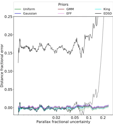
Figure 1 shows the rolling mean (with a window of 20 sources) of the fractional error in the inferred source distances as a function of their parallax fractional uncertainty. Distances were obtained using all our prior families plus the EDSD one, in each case the parallax spatial correlations were included and neglected (shown in the figure as solid and dashed lines, respec-tively). It is clear from this figure that neglecting the paral-lax spatial correlations when using the EDSD prior results in smaller fractional errors than those obtained when the parallax spatial correlations are taken into account, even for high-quality sources. The smaller fractional error results from neglecting the parallax spatial correlations, which is equivalent to assume that the data set is more informative than it is. In general, the more informative the data set is, the less influence the prior has on the posterior. Thus, when parallax spatial correlations are taken into account the mode of the posterior is attracted to the mode of the prior, which is located at 2.7 kpc (corresponding to 2L, with L its length-scale,Bailer-Jones et al. 2018), hence the larger frac-tional error. Since the mode of the cluster oriented prior families is inferred from the data, it results in smaller fractional errors.
Table 1 shows the rms fractional error of the inferred distances for three different ranges of parallax fractional uncer-tainties. In the most precise parallax bin, that of f$ < 0.05,
the Gaussian prior returns the smallest fractional error, followed closely by the King, GMM, EFF, and uniform prior families. This
0.02
0.05
0.1
0.2
Parallax fractional uncertainty
0.00
0.05
0.10
0.15
0.20
0.25
Distance fractional error
Priors
Uniform
Gaussian GMMEFF KingEDSD
Fig. 1.Distance fractional error as a function of parallax fractional
uncertainty. The inference was done using all our prior families (color coded) on a synthetic cluster with 500 stars located at 500 pc. The lines show the rolling mean (computed with a window of 20 sources) of results obtained including (solid line) and neglecting (dashed lines) the parallax spatial correlations.
Table 1. Fractional errors in the source distances.
Prior f$< 0.05 0.05 < f$< 0.1 f$> 0.1 log Z Uniform 6.98(12.36) 8.58(10.67) 10.82(11.16) 103.15 ± 0.16 Gaussian 6.88(11.29) 8.49(8.76) 10.87(10.88) 103.57 ± 0.17 GMM 6.90(11.29) 8.53(8.66) 10.89(10.90) 103.07 ± 0.18 EFF 6.98(11.26) 8.46(8.87) 10.77(10.81) 103.92 ± 0.17 King 6.89(11.28) 8.47(8.72) 10.85(10.90) 104.52 ± 0.15 EDSD 90.29(14.08) 94.73(34.40) 425.59(384.89)
Notes. The columns show the prior family and the rms of the fractional error for three bins of the parallax fractional uncertainty. The number in parenthesis correspond to values obtained when the parallax spatial correlations are neglected. The last column shows the logarithm of the Bayesian evidence computed for each model.
result was expected since the true underlying distribution was Gaussian. In the less precise parallax bins ( f$> 0.05), the
low-est fractional errors are those obtained with the EFF and King prior families. This interesting result shows that our astrophysical prior families produce excellent estimates of the source distances even when they do not match the true underlying distribution. In Table1, the numbers in parentheses correspond to the rms of the fractional errors obtained when the parallax spatial correla-tions are neglected. These values are consistently larger than those obtained when the parallax spatial correlations are included. The only exception being the EDSD prior, for which the decrease in information produces a shift in its mode, as explained above. The lower fractional errors obtained by the cluster oriented prior fam-ilies when the parallax spatial correlations are taken into account
20 0 20 Error [pc] Uniform =-0.72 EFF =-0.75 20 0 20 Error [pc] Gaussian =-0.75 King =-0.75 20 0 20
Offset from centre [pc] 20 0 20 Error [pc] GMM =-0.74 20 0 20
Offset from centre [pc] EDSD
=0.02
0.02 0.04 0.06 0.08 0.10
Parallax fractional uncertainty
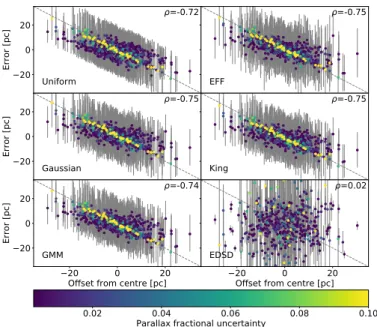
Fig. 2.Error of the estimated source distances as a function of the o
ff-set from the cluster center (i.e., true distance minus cluster location). The panels show the results of different prior families. The color scale indicates the parallax fractional uncertainty and the gray dashed lines show the perfect anti-correlation. The Pearson correlation coefficient is shown on the top-right corner of each panel.
are the result of the proper modeling of the data characteristics. Finally, the last column of Table 1shows the logarithm of the Bayesian evidence computed for each of our cluster oriented prior families (the Bayesian evidence of the EDSD prior cannot be computed since its only parameter remains fixed). These values of the Bayesian evidence are all very similar, and according to the Jeffreys’ scale (see Note9), their resulting Bayes factors pro-vide inconclusive epro-vidence to select one model over the others. Given the previous results, we can safely say that all our cluster-oriented prior families perform well to a similar extent with regard to recovering the source distances.
Despite the good performance of the cluster-oriented prior families, they produce random errors in the source distance esti-mates that are inherent to the quality of the data. In Fig.2, we show for each prior family, the resulting distance error of indi-vidual sources as a function of its true position within the cluster. The distances obtained with all the cluster oriented prior fami-lies include the parallax spatial correlations, however, to make a fair comparison in the case of the EDSD prior they do not take these correlations into account. As can be observed, the distances obtained with the cluster oriented prior families show a clear anti-correlation between their error and the source o ff-set to the cluster center (the Pearson correlation coefficients is shown in the top-right corner of each panel of the figure). In the EDSD prior the correlation is negligible. The anti-correlation in the cluster prior families is proportional to the source fractional uncertainty; sources with large fractional uncertainty tend to fall over the dashed line of slope −1.
The anti-correlation of this error has its origin in the same effect that produces the shift in the posterior distances obtained with the EDSD prior (see Fig.1). In other words, when the par-allax uncertainty is small, the information on the source location is more constraining and the prior plays a minor role. On the other hand, when the parallax uncertainty increases, its infor-mation reduces and the prior becomes more important. In this latter case, the posterior is attracted towards the mode of the
prior, which results in the anti-correlation. From the compari-son of the different prior families we conclude that: (i) the clus-ter oriented prior families show an error that is proportional to the source fractional uncertainty, (ii) the value of this error is smaller than that obtained with the EDSD prior (see Table1). Thus we conclude that the cluster oriented prior families outper-form the EDSD prior when inferring distances to stellar clusters. This comes as a no surprise since the EDSD prior was designed for the entire Galaxy and not for individual clusters. As explicitly mentioned byBailer-Jones (2015), “the exponentially decreas-ing volume density prior may be suitable when lookdecreas-ing well out of the disk, where for a sufficiently deep survey the decrease in stellar density is caused mostly by the Galaxy itself rather than the survey”.
5. Conclusions and future perspectives.
We have made the free and open code Kalkayotl public. It is a statistical tool for the simultaneous inference of star cluster parameters and individual distances of its stars. This tool utilizes distance prior families specifically designed for stellar clusters and takes into account the parallax spatial correlations present in the Gaia data. Upon convergence, Kalkayotl delivers high cred-ibility (>90%) estimates of distances to stellar clusters located closer than ∼5 kpc, and cluster sizes up to ∼1 kpc, with these values depending on the number of cluster stars. The samples from the posterior distributions of both cluster parameters and source distances can be used to propagate their uncertainties into subsequent analyses.
Although the general formalism of our methodology can be applied to parallax measurements of diverse origins, our method-ology is tuned to deal with the parallax spatial correlations of the Gaiadata. It is flexible enough to accommodate different values of parallax zero point and spatial correlation functions.
We validate this tool on realistic synthetic data sets and obtain the following conclusions:
– Distance estimates to sources with large fractional uncertain-ties (>0.05) can have large (>20%) systematic errors under incorrect assumptions. Provided that our assumptions are valid, these low-information sources can still be useful to constrain the cluster population parameters.
– Compared to the inverse mean parallax approach, which results in cluster distance estimates that have low credibil-ity (<80%) but small fractional errors (<5%) for clusters up to ∼1 kpc, and high credibility (>80%) but large fractional errors (>10%) beyond this limit, our methodology returns distance estimates with small fractional errors (<10%) and high credibility (>90%) for clusters up to ∼5 kpc. The excep-tions are the nearest clusters (≤100 pc) and the GMM prior family.
– The stellar distance estimates provided by Kalkayotl show errors that are anti-correlated with the true position of the source relative to the cluster center. The anti-correlation is proportional to the source fractional uncertainty and reaches its maximum (−1) at distances larger than 1 kpc. Nonethe-less, this error is still smaller than that incurred by the EDSD prior.
– The spatial correlations in the parallax measurements are a non-trivial characteristic of Gaia data. Neglecting them has negative consequences at both source and population level, among which, increased fractional errors, underesti-mated uncertainties, and low credibility are to be expected. Our results show that there is no objective reason in terms of accuracy, precision, or computing time to neglect the
parallax spatial correlations when inferring the distances to clusters and its stars.
– The amount of information provided by the data set is not always enough to constraint complex models. Thus we strongly suggest that the users of Kalkayotl start with the simplest prior families (i.e., uniform and Gaussian), ver-ify their convergence, and later on, if needed, move to the more complex ones. If the latter are needed, their perfor-mance or convergence can be improved by reparametrizing: fixing some of the parameters or increasing the informa-tion content of the hyper-parameters. In this sense, users are encouraged to encode, by means of prior families and their hyper-parameters, the information they possess on the spe-cific cluster that they analyze.
Although our methodology represents what we consider is an important improvement in the estimation of distances to stellar clusters from parallax data, it still has several caveats. Among those that we have detected and plan to address in the near future, we cite the following.
– It is assumed that the list of cluster candidate members is not contaminated either biased (Assumption5). However, in practice, this rarely happens. Cluster membership method-ologies have certain true positive and contamination rates (see, e.g.,Olivares et al. 2019). A further improvement of our methodology will be to simultaneously infer the cluster parameters and the degree of contamination while incorpo-rating the selection function.
– The posterior distribution of the cluster distance may be fur-ther constrained by the inclusion of additional observations (e.g., photometry, proper motions, radial velocities, and sky positions). In the future, we plan to include the rest of the Gaiaastrometric observables to further constrain the param-eters of stellar clusters.
Acknowledgements. We thank the anonymous referee for the comments that helped to improve the quality of this manuscript. This research has received fund-ing from the European Research Council (ERC) under the European Union’s Horizon 2020 research and innovation program (Grant agreement No 682903, P. I. H. Bouy), and from the French State in the framework of the “Investments for the future” Program, IdEx Bordeaux, reference ANR-10-IDEX-03-02. L. C. and Y. T. acknowledge support from “programme national de physique stellaire” (PNPS) and from the “programme national cosmologie et galaxies” (PNCG) of CNRS/INSU. The figures presented here were created using Matplotlib (Hunter 2007). Computer time for this study was provided by the computing facilities MCIA (Mésocentre de Calcul Intensif Aquitain) of the Université de Bordeaux
and of the Université de Pau et des Pays de l’Adour. J.O expresses his sincere gratitude to all personnel of the DPAC for providing the exquisite quality of the Gaiadata.
References
Anders, F., Khalatyan, A., Chiappini, C., et al. 2019,A&A, 628, A94
Armstrong, J. J., Wright, N. J., Jeffries, R. D., & Jackson, R. J. 2020,MNRAS, 494, 4794
Astraatmadja, T. L., & Bailer-Jones, C. A. L. 2016,ApJ, 832, 137
Bailer-Jones, C. A. L. 2015,PASP, 127, 994
Bailer-Jones, C. A. L., Rybizki, J., Fouesneau, M., Mantelet, G., & Andrae, R. 2018,AJ, 156, 58
Betancourt, M. J., & Girolami, M. 2013, ArXiv e-prints [arXiv:1312.0906] Bossini, D., Vallenari, A., Bragaglia, A., et al. 2019,A&A, 623, A108
Cantat-Gaudin, T., Vallenari, A., Sordo, R., et al. 2018,A&A, 615, A49
Chabrier, G. 2005, in The Initial Mass Function: From Salpeter 1955 to 2005, eds. E. Corbelli, F. Palla, & H. Zinnecker,Astrophys. Space Sci. Lib., 327, 41
Chan, V. C., & Bovy, J. 2020,MNRAS, 493, 4367
Choi, J., Dotter, A., Conroy, C., et al. 2016,ApJ, 823, 102
Chung, Y., Rabe-Hesketh, S., Dorie, V., Gelman, A., & Liu, J. 2013,
Psychometrika, 78, 685
Dotter, A. 2016,ApJS, 222, 8
Duane, S., Kennedy, A. D., Pendleton, B. J., & Roweth, D. 1987,Phys. Lett. B, 195, 216
Elson, R. A. W., Fall, S. M., & Freeman, K. C. 1987,ApJ, 323, 54
ESA1997,The HIPPARCOS and TYCHO catalogues. Astrometric and photo-metric star catalogues derived from the ESA HIPPARCOS Space Astrometry Mission, ESA Spec. Publ., 1200
Gaia Collaboration (Prusti, T., et al.) 2016,A&A, 595, A1
Gaia Collaboration (van Leeuwen, F., et al.) 2017,A&A, 601, A19
Gaia Collaboration (Brown, A. G. A., et al.) 2018,A&A, 616, A1
Galli, P. A. B., Moraux, E., Bouy, H., et al. 2017,A&A, 598, A48
Galli, P. A. B., Loinard, L., Bouy, H., et al. 2019,A&A, 630, A137
Hunter, J. D. 2007,Comput. Sci. Eng., 9, 90
Jeffreys, H. 1961,Theory of Probability, 3rd edn. (Oxford, England: Oxford) King, I. 1962,AJ, 67, 471
Lindegren, L., Hernández, J., Bombrun, A., et al. 2018,A&A, 616, A2
Luri, X., Brown, A. G. A., Sarro, L. M., et al. 2018,A&A, 616, A9
Morton, T. D. 2015, isochrones: Stellar model grid package (Astrophysics Source Code Library)
Olivares, J., Moraux, E., Sarro, L. M., et al. 2018,A&A, 612, A70
Olivares, J., Bouy, H., Sarro, L. M., et al. 2019,A&A, 625, A115
Palmer, M., Arenou, F., Luri, X., & Masana, E. 2014,A&A, 564, A49
Perren, G. I., Vázquez, R. A., & Piatti, A. E. 2015,A&A, 576, A6
Perren, G. I., Giorgi, E. E., Moitinho, A., et al. 2020,A&A, 637, A95
Perryman, M. A. C., Lindegren, L., Kovalevsky, J., et al. 1997,A&A, 500, 501
Salvatier, J., Wieckiâ, T. V., & Fonnesbeck, C. 2016, PyMC3: Python Probabilistic Programming Framework(Astrophysics Source Code Library) Speagle, J. S. 2020,MNRAS, 493, 3132
Vasiliev, E. 2019,MNRAS, 2030,
Wright, N. J., & Mamajek, E. E. 2018,MNRAS, 476, 381
Appendix A: Bayesian evidence
Here, we provide details of the Kalkayotl subroutine that com-putes the Bayesian evidence of the different prior families. Since PyMC3 does not provide evidence computation we use the python package dynesty (Speagle 2020).
The only purpose of this additional tool is to help the users of Kalkayotl to decide which prior family is the most suitable to describe their data. Since here we are not interested in the dis-tances to the stars, we marginalize them. The following provides the steps and assumptions undertaken in the marginalization of parametersΘ from the posterior distribution (see Eq. (6)). Thus, the marginalization implies that
P(φ | D) ≡ Z P(Θ, φ | D)dΘ (A.1) ∝ Z L(D |Θ) · π(Θ | φ) · ψ(φ)dΘ,
where the proportionality constant Z is the evidence that will be computed. To numerically compute the marginalization integral we made the following assumptions12.
Assumption: the distancesΘ = {θi}Ni=1are independent and
identically distributed with a probability π(θ | φ).
Assumption: the observed parallaxes D = {$i, σ$,i}Ni=1 are
independent (i.e., here, we assume no spatial correlations) and normally distributed N(· | ·).
Under the previous assumptions, we have
P(φ | D)= ψ(φ)· N Y i=1 Z N ($i| T (θi), σ$,i) · π(θi|φ)·dθi. (A.2)
Finally, we approximate each of the N integrals by summing over a M-element {θj}Mj=1of samples from the prior π(φ). Thus,
we have P(φ | D) ≈ ψ(φ) · N Y i=1 1 M M X j=1 N ($i| T (θj), σ$,i). (A.3)
We run dynesty with the following configuration. We use the static Nested sampler with a single bound and a stopping cri-terion of ∆ log Z < 1.0 (seeSpeagle 2020, for more details). To reduce the computing time we take a random sample of only N= 100 cluster stars, always ensuring that this sample remains the same when computing evidence of different models. The M value was set heuristically to 1000 prior samples.
Appendix B: Details of the accuracy and precision
In this section, we present the results obtained after running our methodology using the same prior family that was used to con-struct the synthetic data set. In our analysis, we use the following configuration. We simultaneously infer the cluster parameters and the source distances using the following hyper-parameters (see Sect.2.4): α= [µ, 0.1µ] pc, with µ the distance obtained by inverting the cluster mean parallax, β= 100 pc, γhyp;EFF= [3, 1],
γhyp;King = 10, and δ = [5, 5]. These hyper-parameters produce
weakly informative priors (i.e., the information they provide is smaller than that available) that we expect to cover the diverse cluster information scenarios in which Kalkayotl can be used, 12 We notice that these assumptions are only made for the sole purpose of evidence computation and they do not apply for the rest of Kalkayotl methodology. 0.10 0.05 0.00 0.05 0.10 Fractional error Location Spatial correlations off on 0.0 0.2 0.4 0.6 Scale 0.00 0.05 0.10 0.15 Fractional uncertainty 0.05 0.10 0.15 0.20 0.25 102 103 Distance [pc] 0 20 40 60 80 100 Credibility [%] 102 103 Distance [pc] 0 20 40 60 80 100 Number of sources 100 500 1000
Fig. B.1.Fractional error, fractional uncertainty, and credibility of the
population parameters as a function of distance. The parameters were inferred on the uniform synthetic data sets using its corresponding prior family (i.e., uniform), the colors indicate the number of sources, and the line styles show the cases in which the spatial correlations were included (solid) or were neglected (dashed). The lines show the mean of the ten simulations and the shaded areas its standard deviation.
especially those with weak prior information. In specific cases where more information is available, and thus a more informa-tive prior can be constructed, the performance of our methodol-ogy is expected to improve.
We apply the Kalkayotl methodology to our synthetic data sets using the minimum number of tuning iterations that ensured convergence. It ranged from 1000 for the uniform and Gaussian prior, to 10 000 for the King prior on the farthest clusters. We use 2000 sampling steps and two parallel chains, which amounted to 4000 samples of the posterior distribution. For our purposes, these are enough samples to compute precise estimates (<2%) of the posterior statistics. Central and non-central parametriza-tions were used for the nearby (<500 pc) and far away clusters, respectively. The parallax zero point was set to 0 mas because, as mentioned in Sect. 3, we did not include systematic paral-lax shifts in the generation of synthetic data. For each synthetic cluster, the inference model was run two times, one includes the parallax spatial correlations and the other neglects them. B.1. Population parameters
We now discuss the results obtained at the population level. For each parameter of our cluster prior families, Figs.B.1–B.3
show, as a function of cluster distance, the following indicators: (i) accuracy in the form of fractional error, which is defined as the posterior mean minus the true value divided by the true value, (ii) precision in the form of fractional uncertainty, which is defined as the 95% credible interval divided by the true value, and (iii) credibility, defined as the percentage of synthetic realizations in which the 95% credible interval includes the true value.
0.10 0.05 0.00 0.05 0.10 Fractional error Location Spatial correlations off on 0.0 0.2 0.4 0.6 Scale 0.00 0.05 0.10 0.15 Fractional uncertainty 0.05 0.10 0.15 0.20 0.25 102 103 Distance [pc] 0 20 40 60 80 100 Credibility [%] 102 103 Distance [pc] 0 20 40 60 80 100 Number of sources 100 500 1000
Fig. B.2.Same as Fig.B.1for the Gaussian prior.
The uniform prior family recovers the location parameter with excellent accuracy, the fractional error is smaller than 3%, and its standard deviation <6%. The precision is good with a fractional uncertainty smaller than 15%. The credibility is also good, with more than 80% of the realizations correctly recov-ering the true value. Clusters located at less than 300 pc show an increase in the fractional error of the location parameter with respect to those located at 400–500 pc. This decrease in accuracy results from minor violations to our Assumption 4. Concerning the scale parameter, it is accurately recovered, with fractional errors smaller than 10–20%, only in clusters located closer than 1 kpc, or closer if it has less than 500 sources. The scale precision decreases with distance and improves with the number of sources, as expected. It has large credibility, in the range of 80–90%, only for clusters located closer than 1 kpc. Beyond this limit, the credibility diminishes as a consequence of the large fractional errors. When the parallax spatial correla-tions are neglected, we observe the following aspects. First, the accuracy of both parameters decreases. Nonetheless, the accu-racy in the cluster distances determination is less affected than that of the scale parameter. Second, the precision of both param-eters is underestimated. Third, the credibility of both parame-ters is severely lowered as a consequence of the larger fractional errors and the underestimated uncertainties.
The Gaussian prior family produces similar results to those of the uniform one, with the following differences, however. First, the precision of the scale parameter remains stable for clus-ters up to 400 pc, and its absolute value improves with respect to that obtained with the uniform prior family. Second, when the parallax spatial correlations are neglected the precision of the scale parameter shows better results than in the case of the uni-form prior family. In addition, the credibility of both parameters also increases, in particular for the scale parameter of clusters located closer than 400 pc.
The location and scale parameters of the King prior fam-ily behave in a similar way as those of the Gaussian one. Nonetheless, the scale parameter is determined with lower
pre-0.10 0.05 0.00 0.05 0.10 Fractional error Location Spatial correlations off on 0.0 0.5 1.0 1.5 Scale 0.5 0.0 0.5 1.0 Tidal radius 0.00 0.05 0.10 0.15 Fractional uncertainty 0.2 0.4 0.6 0.8 1.0 0.5 1.0 1.5 102 103 Distance [pc] 0 20 40 60 80 100 Credibility [%] 102 103 Distance [pc] 0 20 40 60 80 100 102 103 Distance [pc] 0 20 40 60 80 100 Number of sources 100 500 1000
Fig. B.3.Same as Fig.B.1but for the King prior family.
cision. Regarding the tidal radius, it is determined with frac-tional errors smaller than 10% only in clusters closer than 500 pc, and with more than 500 sources. Beyond the 500 pc, the results are still credible but noisy, with the errors compensated by the large uncertainties. When the parallax spatial correlations are neglected the results of the location and scale parameters are similar to those of the Gaussian prior family. The tidal radius is underestimated in the region of 300 pc to 2 kpc, and over-estimated beyond 2 kpc. The large fractional error and small uncertainty diminish the parameter’s credibility down to 20% at 1 kpc. The increased credibility at 3–4 kpc results from the large uncertainties.
In the EFF prior family, the location parameter is deter-mined with larger noise and uncertainty, with respect to those of the previous prior families. However, it has credibility larger than 80% for clusters beyond 200 pc. On the contrary, the scale parameter fractional errors are systematically larger, 40% on average. This large and systematic fractional error reduces the scale credibility even in clusters with 500 and 1000 sources. The Gamma parameter also shows systematic fractional errors but towards smaller values, thus resulting in credibilities smaller than 80%. Based on these results we conclude that inferring both the scale and gamma parameters simultaneously produces and non-identifiable model. This can be solved by fixing the gamma parameter to obtain a Cauchy or Plummer distributions, in which the accuracy and precision of their parameters improve to values similar to those of the uniform prior.
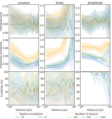
In our analysis of the GMM prior family, we use two com-ponents, which already make it the most complex of our prior families; with three times more parameters than the uniform and Gaussian prior families. Due to this complexity, we faced difficulties in ensuring the convergence of the MCMC algo-rithm in clusters located beyond 1 kpc. Thus, Fig. B.5 shows only those cases in which convergence was warranted. In addi-tion, the figure only shows the results of the closest of the two Gaussian components. As can be observed from this figure, both the location and scale parameters are overestimated by 5–10%
0.10 0.05 0.00 0.05 0.10 Fractional error Location Spatial correlations off on 0.0 0.5 1.0 1.5 Scale 0.4 0.2 0.0 0.2 0.4 Gamma 0.00 0.05 0.10 0.15 Fractional uncertainty 0.2 0.4 0.6 0.8 1.0 0.1 0.2 0.3 0.4 102 103 Distance [pc] 0 20 40 60 80 100 Credibility [%] 102 103 Distance [pc] 0 20 40 60 80 100 102 103 Distance [pc] 0 20 40 60 80 100 Number of sources 100 500 1000
Fig. B.4.Same as Fig.B.1for the EFF prior.
0.00 0.05 0.10 0.15 Fractional error Location Spatial correlations off on 0.0 0.5 1.0 1.5 Scale 0.2 0.1 0.0 0.1 0.2 Amplitude 0.02 0.04 0.06 0.08 Fractional uncertainty 0.2 0.4 0.6 0.8 1.0 0.2 0.4 0.6 102 103 Distance [pc] 0 20 40 60 80 100 Credibility [%] 102 103 Distance [pc] 0 20 40 60 80 100 102 103 Distance [pc] 0 20 40 60 80 100 Number of sources 100 500 1000
Fig. B.5.Same as Fig.B.1for the GMM prior. For the sake of clarity,
only the parameters of the first component in the mixture are shown. Due to convergence issues, the results of clusters beyond 1 kpc are not shown.
and 40–80%, respectively. This overestimation results from the confusion between the components. Due to the symmetry of this model, its components can be interchanged resulting in loca-tions that are overestimated for the closest component and under-estimated for the farthest one. In addition, the scale of both components is overestimated. Despite the issues related to the model symmetry and its lack of identifiability the amplitudes
20
40
60
80
100
Credibility [%]
Spatial correlations
off
on
0.025
0.050
0.075
0.100
0.125
0.150
Fractional RMS
0.05
0.10
0.15
Fractional uncertainty
10
210
3Distance [pc]
1.0
0.8
0.6
0.4
0.2
0.0
Correlation
Number of sources
100
500
1000
Fig. B.6.Results of the uniform prior family. Panels show the
credi-bility, fractional error, fractional uncertainty, and correlation coefficient of source distances as functions of the cluster distance. Captions as in Fig.B.1.
of both components are recovered with low fractional errors and high credibility. The identifiability problem can be partially solved if there is prior information that can be used to break the symmetry13.
B.2. Source distances
We now discuss the performance of our methodology at recov-ering the individual source distances (i.e., those to the cluster stars). FigureB.6 shows, at each cluster distance, the mean of the following indicators: (i) credibility (as defined above), (ii) 13 Further details can be found in https://mc-stan.org/users/
documentation/case-studies/identifying_mixture_models. html
fractional root mean square (rms) error, (iii) fractional uncer-tainty, and (iv) correlation coefficient between the distance error and the offset of the source to the cluster center (more details below). For simplicity, we only show the results obtained with the uniform prior family. The rest of the prior families produce similar results, except for the GMM one, in which the credibility diminishes to 60% for sources in clusters located beyond 700 pc. The credibility of our source distance estimates is higher than 90%, a value that contrasts with that obtained when the parallax spatial correlations are neglected. In this latter case, the credi-bility increases constantly from 30% for the closest clusters to a maximum of 80% for the 3–4 kpc clusters; beyond this lat-ter value, it sinks again. The low credibility obtained when the parallax spatial correlations are neglected is a consequence of the underestimated uncertainties, of both the cluster parameters (see the previous section) and source distances, and the compar-atively large fractional errors.
The fractional rms error remains below the 5% in most of our prior families and almost all cluster distances. The only exceptions are the clusters at 4–5 kpc measured with the EFF and GMM prior families, nonetheless, these have mean frac-tional rms values lower than 8%. This indicator also shows the lowest performance when the parallax spatial correlations are neglected. The difference between the fractional rms error obtained with and without the parallax spatial correlations is negligible for the closest clusters (<500 pc) but grows with dis-tance until it reaches 15% at 5 kpc.
The mean fractional uncertainty shows two distinct regimes. First, for the clusters closer than 1 kpc it remains low at values <3%. Then, it increases with distance and reaches 15% at 5 kpc. The uncertainties of the individual distances are influenced by the cluster size, in the sense that well defined and compact clus-ters produce low uncertainties in the stellar distances. Thus, the two observed regimes in the fractional uncertainty are explained as follows. When the cluster scale is accurately estimated, the uncertainties of the individual distances are driven mainly by the parallax uncertainty, which is the case for clusters up to 1 kpc. However, as soon as the scale parameter is overestimated, which occurs beyond 1 kpc, the uncertainties of the individual distances are driven by both the parallax uncertainty and the cluster scale. Since the latter grows with increasing cluster distance, then the uncertainties of the source distances grow as well. Finally, we observe than neglecting the parallax spatial correlations results in uncertainties that are underestimated with respect to the true model for clusters closer than 700 pc, and then overestimated for the rest of the distances. This behavior of the fractional uncer-tainty results also from the combined influence of the parallax uncertainty itself and the fractional error of the cluster scale. In this case, the fractional error of the latter starts to increase at smaller distances than that observed when the parallax spatial correlations are not neglected (see Fig.B.1).
As discussed in Sect.4.2, the inferred distances to individ-ual sources within a cluster show an error that is anti-correlated with the source position with respect to the cluster center. The value of the anti-correlation coefficient depends on both the par-allax uncertainty and the cluster size. Sources with a parpar-allax uncertainty that produces a posterior distance distribution that is narrower than the cluster size have negligible anti-correlation value. Thus, if the precision in the source distance is smaller than the cluster size, then the source position can be accurately determined within the cluster. On the other hand, sources with increasing parallax uncertainties result in posterior distances that are increasingly dominated by the cluster prior, and by the scale parameter in particular. Thus, the mode of the
poste-rior distribution of these sources is attracted to the mode of the prior. Finally, the distances of sources in the near (far) end of the cluster are over(under)-estimated producing thus the anti-correlated error. In all our prior families, we observe that the anti-correlation coefficient attains its maximum at 1 kpc, and then it either remains constant for the populous clusters or dimin-ishes for the poorest ones. As described in the previous section, 1 kpc is the limit at which we can accurately estimate the cluster sizes. Therefore, the increase in the anti-correlation coefficient is explained by the continuous increase in the parallax uncer-tainty at the constant and accurately determined cluster size. Beyond 1 kpc, the cluster size is overestimated and the anti-correlation stops growing. Neglecting the parallax spatial cor-relations results in a lower anti-correlation coefficient. Although it may seem a desirable effect, it is simply explained by an over-estimated cluster size, which for the purposes of this work, is an undesirable effect.
Our main conclusion from this analysis is that, although source distances obtained when the parallax spatial correlations are taken into account have an anti-correlated error, the value of this error is smaller than that of the distances estimated without the parallax spatial correlations.
Appendix C: Sensitivity to the hyper-parameter values
The inference of model parameters is more influenced by the prior, and therefore sensitive to its hyper-parameter values, under poorly constraining data sets. Thus, we reassess the accuracy, precision, and credibility of both the location and scale param-eters on the less informative of our data sets: those of clus-ters with 100 sources and located at the farthest distances: 1– 5 kpc. In addition, since the scale parameter is only accurately determined at distances closer than 1 kpc, we analyze its sensi-tivity to the hyper-parameter values in clusters at distances of 500–900 pc. For simplicity, we only present the sensitivity anal-ysis performed for the Gaussian prior family.
In Appendices B.1 and B.2 we use α = [µ, 0.1µ], with µ the distance obtained by inverting the cluster mean paral-lax, and β = 100 pc as hyper-parameters of the location and scale parameters, respectively. To evaluate the sensitivity of our methodology to these hyper-parameters, we change their values to α0 = [µ0, 0.1µ0] with µ0 = µ(1 ± 0.1) and β0 = β(1 ± 0.5).
The latter implies evaluating the sensitivity of our methodology to offsets in the hyper-parameter values of 10% in location and 50% in scale. In general, hyper-parameters are often set using the information available a priori. Thus, we chose the previous offset percentages since: (i) we do not expect large variation in the estimates of the cluster distance obtained by simply inverting its mean parallax, and (ii) we do expect considerable variations in the estimates of cluster sizes obtained from the literature (see for example Table 1 ofOlivares et al. 2018).
FigureC.1shows the fractional error, fractional uncertainty, and credibility of the location and scale parameters as a func-tion of distance. As can be observed, the locafunc-tion parameter is insensitive to the change of its hyper-parameter values up to 4 kpc. Beyond this latter value, the variations due to the hyper-parameter values start to be larger than those due to random fluc-tuations (i.e. those introduced by the ten randomly simulated data sets of each cluster). Similarly, the variations in the frac-tional uncertainty due to hyper-parameter values are larger than the random fluctuations only at 4 kpc and beyond. Finally, the credibility of the location parameter is also negligibly affected by the hyper-parameter values since it remains larger than 80%.