HAL Id: hal-00302364
https://hal.archives-ouvertes.fr/hal-00302364
Submitted on 24 Sep 2004
HAL is a multi-disciplinary open access
archive for the deposit and dissemination of
sci-entific research documents, whether they are
pub-lished or not. The documents may come from
teaching and research institutions in France or
abroad, or from public or private research centers.
L’archive ouverte pluridisciplinaire HAL, est
destinée au dépôt et à la diffusion de documents
scientifiques de niveau recherche, publiés ou non,
émanant des établissements d’enseignement et de
recherche français ou étrangers, des laboratoires
publics ou privés.
A non-linear and stochastic response surface method for
Bayesian estimation of uncertainty in soil moisture
simulation from a land surface model
F. Hossain, E. N. Anagnostou, K.-H. Lee
To cite this version:
F. Hossain, E. N. Anagnostou, K.-H. Lee. A non-linear and stochastic response surface method for
Bayesian estimation of uncertainty in soil moisture simulation from a land surface model. Nonlinear
Processes in Geophysics, European Geosciences Union (EGU), 2004, 11 (4), pp.427-440. �hal-00302364�
in Geophysics
© European Geosciences Union 2004
A non-linear and stochastic response surface method for Bayesian
estimation of uncertainty in soil moisture simulation from a land
surface model
F. Hossain, E. N. Anagnostou, and K.-H. Lee
University of Connecticut, Department of Civil and Environmental Engineering, Storrs, Connecticut, USA Received: 16 March 2004 – Revised: 30 June 2004 – Accepted: 12 July 2004 – Published: 24 September 2004
Part of Special Issue “Nonlinear deterministic dynamics in hydrologic systems: present activities and future challenges”
Abstract. This study presents a simple and efficient scheme
for Bayesian estimation of uncertainty in soil moisture simu-lation by a Land Surface Model (LSM). The scheme is as-sessed within a Monte Carlo (MC) simulation framework based on the Generalized Likelihood Uncertainty Estima-tion (GLUE) methodology. A primary limitaEstima-tion of using the GLUE method is the prohibitive computational burden imposed by uniform random sampling of the model’s pa-rameter distributions. Sampling is improved in the proposed scheme by stochastic modeling of the parameters’ response surface that recognizes the non-linear deterministic behav-ior between soil moisture and land surface parameters. Un-certainty in soil moisture simulation (model output) is ap-proximated through a Hermite polynomial chaos expansion of normal random variables that represent the model’s pa-rameter (model input) uncertainty. The unknown coefficients of the polynomial are calculated using limited number of model simulation runs. The calibrated polynomial is then used as a fast-running proxy to the slower-running LSM to predict the degree of representativeness of a randomly sam-pled model parameter set. An evaluation of the scheme’s efficiency in sampling is made through comparison with the fully random MC sampling (the norm for GLUE) and the nearest-neighborhood sampling technique. The scheme was able to reduce computational burden of random MC sam-pling for GLUE in the ranges of 10%–70%. The scheme was also found to be about 10% more efficient than the nearest-neighborhood sampling method in predicting a sampled pa-rameter set’s degree of representativeness. The GLUE based on the proposed sampling scheme did not alter the essential features of the uncertainty structure in soil moisture simula-tion. The scheme can potentially make GLUE uncertainty estimation for any LSM more efficient as it does not impose any additional structural or distributional assumptions.
Correspondence to: E. N. Anagnostou
1 Introduction
In hydrology, uncertainty estimation techniques that are based on fully random Monte Carlo (MC) sampling of probability distributions are usually considered the preferred method due to their lack of restrictive assumptions, com-pleteness in sampling the error structure of the random vari-ables, and the increasing availability of computational re-sources (Beven and Freer, 2001; Beck, 1987; Kremer, 1983). MC sampling can also bypass several limitations of analyt-ical techniques (Bras and Rodriguez-Iturbe, 1993). An un-certainty estimation technique called Generalized Likelihood Uncertainty Estimation (GLUE) (Beven and Binley, 1992) is one such MC based tool that can be employed to assess an en-vironmental model’s predictive uncertainty. This method ex-tends the type of Generalized Sensitivity Analysis (GSA) of Spear and Hornberger (1980) by evaluating the simulation re-sults for each randomly sampled model parameter set against some observed data through a likelihood value. Because its structure is rooted in Bayesian theory, GLUE also allows blending of prior and current information for improved a pos-teriori inferences. While GLUE is not the only uncertainty assessment tool currently available (Misirli et al., 2003; Thie-mann et al., 2001; Tyagi and Haan, 2001; Krzysztofowicz, 2000; Young and Beven, 1994), the simplicity of the the-ory behind the technique is what makes it convenient and very easy to implement (Beven and Freer, 2001). GLUE has therefore found extensive application in the assessment of predictive uncertainty of many hydrologic variables like streamflow, flood inundation, ground water flow, land surface fluxes, etc. (Schulz and Beven, 2003; Christaens and Feyen, 2002; Beven and Freer, 2001; Schulz et al., 2001; Romanow-icz and Beven, 1998; Franks et al., 1998; Franks and Beven, 1997; Freer et al., 1996; among many others). Recently, the GLUE technique has also proved to be a powerful tool in un-derstanding the implications of remotely sensed rainfall error adjustment on flood prediction uncertainty (Hossain et al., 2004).
428 F. Hossain et al.: A non-linear and stochastic response surface method However, the GLUE method has a major drawback. It
requires analysis of multiple simulation scenarios based on uniform random sampling of the model parameter hyper-space. This requirement can be computationally prohibitive for physically complex models that are slow-running (Bates and Campbell, 2001; Beven and Binley, 1992). Beven and Binley (1992) have argued in detail that the assumption of uniform distribution is unlikely to prove critical for GLUE. Freer et al. (1996) have further justified uniform sampling because it makes the GLUE procedure simple to implement and avoids the necessity to sample from some multivariate set of correlated distributions which is often very difficult to justify from observed data. Nevertheless, the drawback of uniformity assumption in GLUE magnifies tremendously for physically complex Land Surface Models (LSM) that simul-taneously balance water and energy budget across the land surface. Thus, GLUE application for Bayesian estimation of uncertainty in land surface-atmosphere flux predictions has so far been limited to relatively simpler conceptualizations of soil-vegetation-atmosphere transfer (SVAT) schemes (e.g. Schulz and Beven, 2003; Schulz et al., 2001; Franks et al., 1998; Franks and Beven, 1997). A more realistic Bayesian assessment of uncertainty requires the application of GLUE to physically complex operational LSMs such as Common Land Model (CLM; Dai et al., 2003), NOAH-LSM (Pan and Mahrt, 1987), BATS (Dickinson et al., 1986) or SiB (Sellers et al., 1986). Uncertainty assessment of these models are important because, despite their physical complexity, they nevertheless suffer from parameter equifinality where a wide range of parameter sets exhibit equally acceptable simula-tions against data available.
In the last decade, researchers have strived to develop nu-merical schemes for efficient sensitivity analyses of LSM pa-rameters. Henderson-Sellers (1993) proposed a Factorial As-sessment (FA) of sensitivity of model parameters that incor-porates the multifactor interactions and tries to avoid the po-tential weakness of the classical sensitivity analyses of per-turbing one parameter at a time. However, the FA method suffers from the following limiting requirements: 1) prior knowledge of parameter variances; and 2) large number of model perturbations (Gao et al., 1996). Collins and Avis-sar (1994) proposed a Fourier Amplitude Sensitivity Test (FAST) for land surface parameters. This method also has drawbacks similar to the FA method with the additional re-quirement that parameters be physically uncorrelated. Gao et al. (1996) summarized that there was no perfect method for characterizing parameter uncertainty of land surface sys-tems and proposed a special form of the classical stand-alone sensitivity analyses for land-surface schemes. Our qualita-tive assessment of the techniques reported in literature and alluded herein indicates that none of them are pertinent to GLUE for making uncertainty estimation of LSMs computa-tionally more efficient.
In recognition of the uncertainty due to input land sur-face parameters and the ease of implementation of the GLUE method, there is a need to develop a parameter sampling tech-nique that can make the application of GLUE more efficient
for LSMs. Such a technique should not impose additional structural or distributional assumptions that may otherwise compromise the inherent simplicity of the GLUE method. Kuczera and Parent (1998) and Bates and Campbell (2001) have already explored the use of Markov Chain Monte Carlo (MCMC) methods for more efficient parameter uncertainty analyses. Bates and Campbell (2001) however reported that MCMC methods cannot be used as a black box – consider-able care is required in its implementation when models have large number of parameters. A further criticism made by Beven and Freer (2001) was that MCMC methods can rarely be useful in making considerable savings in computing time when the model response surface with respect to parameters is not well defined and has the presence of multiple local maxima or plateau. Christaens and Feyen (2002) employed the Latin Hypercube Sampling (LHS) method to accelerate parameter sampling for the MIKE-SHE hydrologic model. However, LHS is based on the assumption of monotonicity of model output in terms of input parameters, in order to be un-conditionally guaranteed of accuracy with an order of mag-nitude fewer runs than uniform random sampling (McKay et al., 1979; Iman et al., 1981). Recent study by Hossain et al. (2004a)1has clearly shown that the use of LHS method is not always effective and that it requires care in planning an effective sampling strategy. Consequently this study is moti-vated by the need to develop a simple but efficient parame-ter sampling technique that can make GLUE computationally more efficient for slow-running LSMs.
In the current state of the art, GLUE for such models would require an interpolator for the model parameter-output response surface. This interpolator could then act as a fast-running proxy to the slow fast-running model and potentially identify the regions of high likelihood values (i.e. regions of high degree of representativeness of the hydrologic system) on the parameter-output response surface. In this study we have chosen to develop a stochastic interpolator based on the “Theory of Homogeneous Chaos” (Wiener, 1938) (hereafter called “interpolator”). We do not demonstrate the presence or absence of chaotic behavior of simulations in this study. However, we are encouraged by the recent well-documented discovery of chaos in hydrologic systems (Sivakumar et al., 2001a and 2001b; Sivakumar, 2000; Jayawardena and Lai, 1994; Rodriguez-Iturbe et al., 1991). Essential concepts of the interpolator are inferred from an uncertainty estimation tool originally developed by Isukapalli et al. (2000). How-ever, the critical evaluation presented herein of the interpo-lator within the GLUE framework for improving parameter sampling is considered a relatively unexplored topic. In this study we make an evaluation of the interpolator on a dif-ferent surface hydrologic variable – soil moisture – which is simulated by the physically-based NOAH-LSM (Pan and Mahrt, 1987). The interpolator is also compared with the
1Hossain, F., Anagnostou, E. N., and Bagtzoglou, A. C.: On Latin Hypercube Sampling for Efficient Uncertainty Estimation of Satellite-derived runoff predictions. J. of Hydrology, in review, 2004.
1 2 3 4 5 6 7 8 9 10 11 12 Month 0.7 0.8 0.9 1 1.1 Bias
Unadjusted Vegetation Parameters Adjusted Vegetation Parameters
0.2 0.25 0.3 0.35 0.4
Vol. Soil Moisture
Observed NOAH (Unadjusted) NOAH (Adjusted) 0 50 100 150 200 Precipitation (mm)
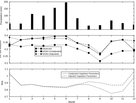
Fig. 1. NOAH-LSM vegetation parameter and bias adjustment for soil moisture simulation. Upper panel – monthly accumulated precipitation
(mm) for 1998. Middle panel – observed soil moisture measurements (mean monthly) at 5 cm depth compared with simulations with adjustments and no adjustments. Lower panel – the monthly multiplicative bias in simulation with adjusted and unadjusted vegetation parameters. Effective study period was 1 March – 30 November 1998.
fully random MC sampling technique (the norm for GLUE) and the nearest-neighborhood parameter sampling technique originally proposed by Beven and Binley (1992).
The study is organized in the following manner. In Sect. 2, a brief description of the study region and data are provided. Section 3 describes the LSM part a and its readjustment part b that were found necessary to make the model representa-tive of the study region. In Sect. 4, we describe the GLUE method based on fully random uniform parameter sampling. Section 5 provides description of the algorithm for the inter-polator for parameter sampling. Section 6 describes the sim-ulation framework for assessment of the interpolator. Sec-tion 7 discusses the results, while Sect. 8 presents the con-clusions and further extensions that can potentially extend the capabilities of the interpolator.
2 Study region and data
Our study region was Northern Illinois (USA) in a farmland in Champaign located 40.01◦N and 88.37◦W. The site
char-acteristics were typical of those found throughout Midwest-ern US with most of the land in agricultural production. The soil was silt loam with a bulk density of 1.5 gm/cm3. The year under study was 1998 when soybeans were planted in the farm. Atmospheric and radiation forcing data from a flux measuring system installed in the farm was recorded ev-ery 30 min for that year. The major atmospheric data com-prised precipitation, temperature, humidity, surface pressure and wind. The radiation forcing data pertained to down-ward solar (short-wave) and downdown-ward long-wave radiation
flux measurements. This data is public domain and avail-able as part of standardized testing protocols for simulation codes of the NOAH-LSM (discussed next). To reduce the im-pact of snow and sensitivity to initial conditions in our study, we chose an effective study period ranging from 1 March – 30 November 1998. For more information on the study re-gion and data measurement protocols the reader is referred to the User’s Guide, Public Release Version 2.5 available at ftp://ftp.emc.noaa.gov/mmb/gcp/ldas/noahlsm/ver 2.5.
3 The land surface model
3.1 Model description
The LSM used in this study was NOAH-LSM (also known as The Community NOAH-LSM) (Pan and Mahrt, 1987). We chose NOAH-LSM as it is a popular operational model and insights into this study could prove beneficial in understand-ing the utility of the proposed samplunderstand-ing technique for uncer-tainty prediction of land surface variables in general. This LSM is a stand-alone, uncoupled, 1-D column version used to execute single-site land surface simulations. In this tra-ditional 1-D uncoupled mode, near surface atmospheric and radiation forcing data are required as input forcing. NOAH-LSM simulates soil moisture (both liquid and frozen), soil temperature, snow pack, depth, snow pack water equivalent, canopy water content and the energy and water flux terms in terms of the surface energy balance and surface water balance. A four-layer soil configuration (comprising a to-tal depth of 2 m) is adopted in the NOAH-LSM for
captur-430 F. Hossain et al.: A non-linear and stochastic response surface method 1 2 3 4 5 6 7 8 9 10 11 12 Month 0 0.2 0.4 0.6 0.8 1
Fraction of Green Vegetation
Unadjusted (Large−scale representation) Adjusted (point−scale representation)
Growing Stage
Flowering Stage
Yielding Stage
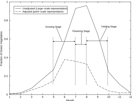
Fig. 2. Readjustment of monthly Fraction of Vegetation parameters for NOAH-LSM to make them more representative of the study region and
point-scale simulation of soil moisture for the upper 5 cm layer. Unadjusted parameters are derived from Normalized Difference Vegetation Index (NDVI; Gutman and Ignatov, 1998). The growth sequence applies for soybeans that were planted during 1998.
ing daily, weekly and seasonal evolution of soil moisture and mitigating possible truncation error in discretization (Srid-har et al., 2002). The lower 1 m acts as gravity drainage at the bottom, and the upper 1meter of soil serves as root zone depth. Since this study concerns the assessment of a param-eter sampling technique, we have considered soil moisture observations and simulations only at the 5 cm depth for the sake of simplicity. For more details on the physical descrip-tion of the model, one may refer to Sridhar et al. (2002). 3.2 Model readjustment
Our preliminary investigation with NOAH-LSM revealed significant underestimation of soil moisture simulation at the 5 cm depth. This thereby indicated an overestimation of Evapotranspiration (ET) process that magnified further dur-ing the soybean growdur-ing season (see Fig. 1, lower panel). We therefore found it necessary to adjust some of the NOAH-LSM vegetation parameters to make the model more rep-resentative of the point-scale soil moisture flux simulations at the farm. We reduced the number of root layers from 3 (100 cm of deep roots) to 2 (40 cm of deep roots). This reduction was justified for our study period, as soybeans do not typically grow roots beyond 30 cm depth (Norman, 1978; Liu, 1997). We found Leaf Area Index (LAI) to be an insensitive parameter to the bias in soil moisture simula-tion. We further hypothesized that a typical soybeans lateral spacing of 80 cm (inferred from: Norman, 1978) should not yield the fraction of green vegetation greater than 0.5 dur-ing the growdur-ing months. The vegetation fraction parame-ters used in LSMs are derived from the NDVI (Normalized Difference Vegetation Index) proposed by Gutman and
Ig-natov (1998). Because NDVI as derived from the NOAA AVHRR are typically representative for the 15×15 km2 res-olution (see Gutman and Ignatov, 1998), we argue that they may require minor adjustment for the point scale study con-ducted herein. The use of high resolution LANDSAT data (30 m) could perhaps address this limitation. However, the non-availability of such higher resolution data prompted us to assume an adjusted set of fraction of vegetation parame-ter for a 1-D (point) investigation scenario. We argue that this assumption is acceptable as the objective of this study is confined to the exploration of sampling efficiency of our pro-posed scheme. Based on knowledge of the soybean growth sequence (i.e. plant in May; flower in July and harvest in October) (Liu, 1997), we adjusted the vegetation fraction pa-rameters as shown in Fig. 2. It is seen that the bias is now reduced after this adjustment for the growing season (May– July). The mean multiplicative bias (ratio of simulated to ob-served) for the effective study period (1 March – 30 Novem-ber 1998) was found to be 0.868 (Fig. 1, lower panel). We therefore applied a final multiplicative bias adjustment fac-tor to the NOAH-LSM soil moisture simulations of 1.15 (i.e. 1/0.868). The effect of bias adjustment after the vegetation parameter fine-tuning is shown to improve simulations sig-nificantly (see Fig. 1, middle panel, dashed line).
3.3 Model parameter uncertainty
NOAH-LSM parameter uncertainty was accounted for the following five soil hydraulic parameters that we consid-ered most sensitive to soil moisture simulation: 1) max-imum volumetric soil moisture content (porosity) (SMC-MAX, m3/m3); 2) saturated matric potential (PSISAT, m) (3)
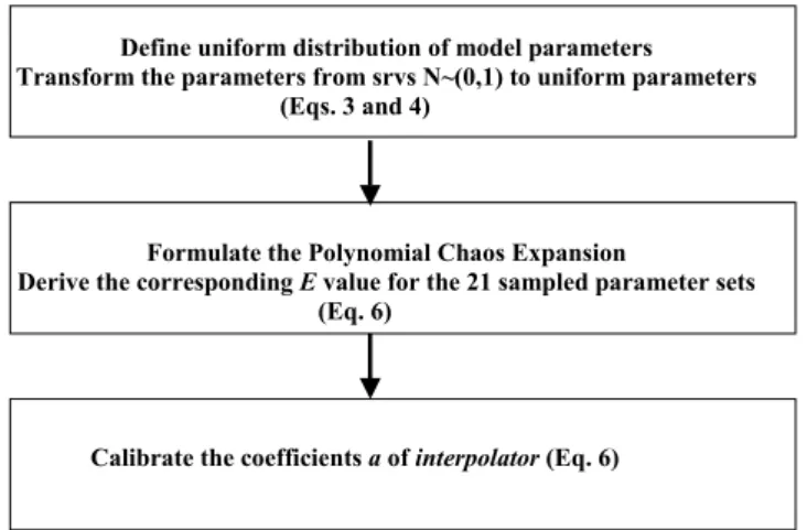
Table 1. Uncertainty ranges for soil hydraulic parameters of NOAH-LSM.
Parameter Minimum value Maximum value Sampling strategy 1. SMCMAX (m3/m3) 0.05 0.50 Uniform 2. PSISAT (m) 0.01 0.65 Uniform 3. SATDK (m/s) 1.00×10⁻⁶ 1.77×10⁻⁴ Log (uniform)
4. BB 2.00 15.00 Uniform
5. SMCWLT (m3/m3) 0.01 0.20 Uniform
saturated hydraulic conductivity K (SATDK, m s−1); 3) pa-rameter ‘B’ of soil-water retention model of Clapp and Horn-berger (1978) (BB); and (4) soil moisture wilting point at which ET ceases (SMCWLT, m3/m3). The parameter un-certainty ranges are shown in Table 1 and were based on the empirical study of Clapp and Hornberger (1978) and the sampling requirements of GLUE (Beven and Binley, 1992) (discussed next).
4 The GLUE methodology
GLUE is based on MC simulation: a large number of model runs are made, each with random parameter values selected from uniform probability distributions for each parameter. The acceptability of each run is assessed by comparing pre-dicted to observed hydrologic measurement through some chosen likelihood measure. Runs that achieve a likelihood below a certain threshold may then be rejected as non-behavioral. The likelihoods of these non-behavioral param-eters are set to zero and are thereby removed from the sub-sequent analysis. Following the rejection of non-behavioral runs, the likelihood weights of the retained (i.e. behavioral) runs are rescaled so that their cumulative total is one (Freer et al., 1996). In this study the GLUE method was applied to uncertainty estimation of soil moisture simulation by NOAH-LSM at the 5 cm depth. Thus at each time step (at 30 minute intervals), the predicted soil moisture from the behavioral runs are likelihood weighted and ranked to form a cumula-tive distribution of soil moisture simulation from which cho-sen quantiles can be selected to reprecho-sent model uncertainty. While GLUE is based on a Bayesian conditioning approach, the likelihood measure is achieved through a goodness of fit criterion as a substitute for a more traditional likelihood func-tion. We have considered two specific likelihood measures in this study: 1) the classical index of efficiency, ENS(Nash
and Sutcliffe, 1970) (Eq. 1), and 2) the exponential index of efficiency,EEXP(Eq. 2).
ENS= " 1 − σ 2 e σobs2 # (1) EEXP =exp " −σe2 σobs2 # , (2)
where σe is the variance of errors and σobs, the variance of
observations. These two likelihood measures are consistent with the requirements of the GLUE method, as both increase monotonically with the similarity of behavior. The purpose of using two different likelihood measures was to demon-strate that the applicability of the interpolator was not sensi-tive to the subjecsensi-tive choice.
Now, to implement the GLUE methodology, each param-eter of NOAH-LSM was specified a range of possible values shown earlier in Table 1. Constant (calibrated) values for all other NOAH-LSM parameters were used. Model predic-tions of soil moisture were carried out, and the model likeli-hood measure was calculated using the efficiency indices of Eqs. (1) and (2). From the specified parameter ranges, MC simulations were conducted that allowed the selection of a large number of behavioral parameter sets characterized by a simulation efficiency index value greater than an assigned minimum threshold value. For further details on GLUE im-plementation, one is referred to Beven and Binley (1992), Freer et al. (1996) and Beven and Freer (2001).
5 Algorithm of the inperpolator
The principle of the interpolator is founded on the “Theory of Homogeneous Chaos” (Wiener, 1938). Wiener (1938) has shown that if deterministic dynamical model is highly non-linear (with a tendency to exhibit chaotic behavior), then it is possible to approximate both inputs and outputs (treated here as random processes) of the uncertain model through series expansion of standard random variables using Hermite Poly-nomials. Although the presence of chaotic behavior in the hydrologic system under study is not addressed herein, re-cent literature supports the wisdom of choosing the “Theory of Homogeneous Chaos” as a basis for formulation of the interpolator (Sivakumar, 2000; Sivakumar et al., 2001a, b; Rodriguez-Iturbe et al., 1991). Rodriguez-Iturbe et al. (1991) has demonstrated chaotic behavior of soil moisture dynamics at seasonal time scales. Since our effective study period was seasonal (from March to November 1998), this observation by Rodriguez-Iturbe et al. (1991) therefore justifies the use of a chaotic approach for our methodology. Furthermore, the re-quirement of multiple ordinary non-linear differential equa-tions as the necessary condition for chaotic behavior in soil moisture dynamics has also been noted by Rodriguez-Iturbe
432 F. Hossain et al.: A non-linear and stochastic response surface method
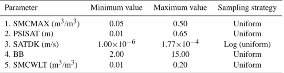
Define uniform distribution of model parameters Transform the parameters from srvs N~(0,1) to uniform parameters
(Eqs. 3 and 4)
Formulate the Polynomial Chaos Expansion
Derive the corresponding E value for the 21 sampled parameter sets (Eq. 6)
Calibrate the coefficients a of interpolator (Eq. 6)
Fig. 3. Flow-chart for the algorithm of the interpolator.
et al. (1991). The physical formulation of NOAH-LSM indi-cates that there are sufficient physical sub-models linking the 5 soil hydraulic parameters (of Table 1) to intuitively expect a chaotic behavior relationship (between soil moisture pre-diction the hydraulic parameters). These notable sub-models are as follows: 1) The prognostic equation for volumetric soil water content (Richards Equation) (Sridhar et al., 2002); 2) The diffusion equation for soil temperature (Sridhar et al., 2002); 3) The Penman-based energy balance approach for potential evaporation (Sridhar et al., 2002); and, 4) The Mahrt and Ek (1984) formulation of surface skin tempera-ture. There are three major steps involved in the algorithm formulation of this interpolator. We describe these steps be-low. For more details the reader is referred to Isukapalli and Georogopolous (1999) and Isukapalli et al. (2000).
5.1 Step one: transformation of parameter distributions Our NOAH-LSM model input parameter uncertainty domain is represented by a 5-D hypercube (Table 1) with the distribu-tion of each parameter being uniform (the norm for GLUE). It is defined as follows,
Xi∼U (pi, qi), i=1, . . . ., 5, (3)
where p and q form the lower and upper parameter ranges (column 1 of Table 1). Subscript i refers to the specific pa-rameter type (from 1 to 5 as listed in Table 1). X represents the parameter value. These uniformly distributed parameters are then expressed as a series of a standard normal random variable (srv) as, xi,j=pi +(qi−pi)( 1 2+ 1 2erf (εi,j/ p 2)) , i=1, . . ., 5, (4) where ε is a srv∼ N(0,1) and j denotes the index for a ran-dom realization. erf (xx) is the error function defined by the following integral, erf (xx)=√2 π xx Z 0 e−w2dw. (5)
In Eq. (5), xx is the srv and w an intrinsic independent vari-able of the error function.
We have now expressed the random inputs (uniformly dis-tributed model parameters) via srv’s as {ε}ni=1 (where, n= 5). The choice of transforming the model parameters to the normal srvs is justified by mathematical tractability of functions of these srv’s (Devroye, 1986).For example, other common univariate distributions such as gamma, exponen-tial, Weibull, log-normal can all be transformed explicitly to normal srv’s.
5.2 Step two: polynomial chaos expansion
Next, we represent our uncertain model output, L – the like-lihood measure (left-hand side of Eqs. 1 or 2), as an n-th order expansion of a Hermite Polynomial of srv’s. This step, called “Polynomial Chaos Expansion”, follows from Ghanem and Spanos (1991). In this study we have consid-ered second order expansion which is defined as follows,
L2=a0,2+ Xn i=1ai,2εi+ n X i=1 aii,2(εi2−1)+ n−1 X i=1 n X j >1 aij,2εiεj, (6)
where the subscript after L represents the order of the expan-sion.
5.3 Step three: calibration of coefficients of the Interpola-tor
From the above Eq. (5), it can be seen that the number of un-known coefficients (the a’s in the right hand side) to be deter-mined for second order polynomial chaos expansion are 21. These unknown coefficients are now identified by generating the same number of model data points and solving the sys-tem of linear algebraic equations. Isukapalli and Georgopou-los (1999) provide guidelines on choosing model points for robust calibration of coefficients. The choice of the model points in this study is, however, left open to the user depend-ing on the nature of the problem. We investigated this issue herein and report our findings in the next section. For calibra-tion of polynomial coefficients we used the Singular Value Decomposition (SVD) (Press et al., 1999) because of its abil-ity to handle ill-conditioned matrices (Press et al., 1999; Hos-sain and Anagnostou, 2004).
In Fig. 3 we summarize the algorithm for the interpola-tor. First, we generate a set of uniformly distributed model parameter sets from srvs (using Eqs. 3, 4 and Table 1). 21 points on the NOAH-LSM’s parameter-output (E) response surface are then chosen. The interpolator is then calibrated for its 21 coefficient values by solving the system of 21 lin-ear algebraic equations. For a more global selection of cali-bration points, we derive 3 different sets of calibrated poly-nomials for the interpolators. The mean E value predicted by the 3 calibrated interpolators is then defined as the most likely E value for a sampled parameter set. The total num-ber of different sets of calibration points required is consid-ered subjective and depends on the nature of the sampling
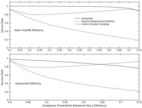
0.4 0.45 0.5 0.55 0.6 0.65 0.7 0.75 Acceptance Threshold for Behavioral Sets (>Efficiency)
0 0.2 0.4 0.6 0.8 1 Success Ratio 0.1 0.15 0.2 0.25 0.3 0.35 0.4 0.45 0.5 0.55 0.6 0.65 0.7 0.75 0 0.2 0.4 0.6 0.8 1 Succes Ratio Interpolator
Nearest Neighbourhood Method Uniform Random Sampling
Exponential Efficiency Nash−Sutcliffe Efficiency
Fig. 4. General comparison of interpolator with Nearest-neighborhood (N N ) method and uniform random sampling as a predictor for
sampled parameter sets in terms of Success Ratio.
problem. Herein we consider 3 sets as sufficient to yield ef-fective results for a 5-D parameter hyperspace. Once the in-terpolator(s) is calibrated for NOAH-LSM on data available, we test its efficiency in parameter sampling in the follow-ing 4 steps: (i) samplfollow-ing N (0, 1) srvs; (ii) generatfollow-ing the corresponding family of uniformly distributed NOAH-LSM parameters from Eq. (4); (iii) computing the mean of the 3 interpolator-predicted E values from Eq. (6); (iv) if the in-terpolator predicts a sampled parameter set to be behavioral, then testing its accuracy by actual execution of NOAH-LSM for that sampled parameter set. Note that the use of the inter-polator in this fashion within the GLUE framework does not violate the fundamental requirement that parameters be sam-pled uniform distributions. It only helps to make an informed decision on sampling by providing an indication of whether the sampled parameter set is behavioral or non-behavioral before making the actual NOAH-LSM model run.
6 Simulation framework
The interpolator (which is now a simple algebraic equation) is potentially a 5–6 orders faster in computation than NOAH-LSM and can therefore serve as a fast-running proxy for making Bayesian decisions on the degree of representative-ness of sampled parameter sets for GLUE analysis. In al-most all previous GLUE applications, behavioral and non-behavioral parameter sets were identified through the actual time-consuming execution of the physically-complex model. This often resulted in high wastage of computational time as the majority of the runs were found to be non-behavioral (see Christaens and Feyen, 2002, for example). In this
sim-ulation framework we tested the accuracy of the interpolator in stochastic modeling the parameter-output response surface for GLUE and assessed its potential in reducing the wastage of computational time due to the non-behavioral runs.
We conducted a total of 500 000 NOAH-LSM simulations by sampling the same number of parameter sets randomly from the ranges in Table 1. This ensemble was further di-vided into 100 sub-divisions each containing 5000 parameter sets. Each of these sets had its respective “true” model re-sponse in terms of likelihood measures (ENSand EEXPfrom
Eqs. (1) and (2), respectively) determined from actual execu-tion of NOAH-LSM. We then evaluated the sampling accu-racy of the interpolator calibrated within each of these 100 sub-divisions to make generalizations on the mean and vari-ability of its performance as a fast-running proxy. We first present a confusion matrix for sampled parameter sets be-low for the interpolator to define the performance measures whose description follows next.
Truth (from NOAH-LSM)
Behavioral Non-behavioral NA NB NC ND Prediction (from interpolator) Non -behavioral Behavioral
434 F. Hossain et al.: A non-linear and stochastic response surface method To define the probability of interpolator to successfully
predict whether a sampled parameter set is behavioral or non-behavioral (based on a given threshold for likelihood mea-sure L) we define Success Ratio (SR) as,
SR = NA NA+NB
(7) The SR indicates only a partial assessment of sampling ef-ficiency. There can be instances where the interpolator is overly conservative in predicting a set as behavioral and thereby achieves a spuriously high SR over very small sam-ples of model executions. Thus, another measure, (BS, Eq. 8) was also defined. BS quantifies the propensity of the interpolator to predict the behavioral sets as non-behavioral or missing regions of high likelihood values on the response surface.
BS = NA+NB NA+NC
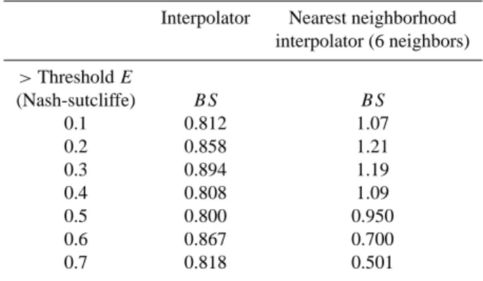
(8) A BS value of less than 1 would indicate that the interpolator has a tendency to be conservative in predicting correctly a sampled parameter set’s likelihood value. A BS value greater than 1 would indicate the interpolator’s propensity to predict samples as behavioral. An ideal interpolator should therefore have a BS of near 1.0 and SR that is higher than that for uniform sampling.
Performance of the interpolator was compared with the fully uniform sampling of parameter sets using the above 2 measures (Eqs. 7 and 8). The Nearest-Neighborhood (N N ) search for interpolating parameter set’s likelihood value was also compared herein (hereafter called N N method). This type of sampling method was first introduced by Beven and Binley (1992) to address the computational concerns of the GLUE method. In the N N method, a sampled point in pa-rameter hyperspace is searched for the “n” nearest neigh-boring points in a model’s response surface that is constructed from a finite number sample points (=1000 pre-constructed model points in this study). The probable like-lihood value is then interpolated by the inverse squared dis-tance technique. We have considered 6, 12 and 24 neigh-bors for the N N method. A point to note is that the N N method requires a computationally intensive sorting algo-rithm to rank all the distances from a sampled point in param-eter hyperspace. The computing time for sorting increases as
N2where N is the size of the pre-constructed model points (Press et al., 1999). Hence a compromise is needed with the size of the pre-constructed model points when the dimension of the parameter hyperspace is high. This is considered a major weakness of the N N method when compared to the interpolator.
7 Results and discussion
In Fig. 4 we show the mean SR values of the 100 sub-divisions (comprising the total 500 000 sets) for the interpo-lator, N N method (6 neighbors) and uniform random sam-pling for two different likelihood measures (Nash-Sutcliffe
Table 2. Mean Bias Score (BS) values for the interpolator and N N
scheme.
Interpolator Nearest neighborhood interpolator (6 neighbors) >Threshold E (Nash-sutcliffe) BS BS 0.1 0.812 1.07 0.2 0.858 1.21 0.3 0.894 1.19 0.4 0.808 1.09 0.5 0.800 0.950 0.6 0.867 0.700 0.7 0.818 0.501
efficiency – upper panel; Exponential efficiency – lower panel). Note that the (1−SR) value actually represents the wastage of computational time due to non-behavioral runs of NOAH-LSM. This is because the sampled parameter sets were evaluated of their degree of representativeness by run-ning the NOAH-LSM only after the prediction by the inter-polator or the N N method gave a strong indication of the set to be behavioral. The interpolator in Fig. 4 was calibrated with sample points that had a minimum E value of 0.7. We observe that the fully uniform random sampling can be very inefficient and result in high wastage of computational time (ranging from 50%–80%) as the acceptance criterion for be-havioral parameter sets increases (ENS>0.4, upper panel;
EEXP>0.5, lower panel). This observation justifies the
wis-dom of using a more efficient parameter sampling scheme for GLUE based on interpolation of the parameter response surface. The interpolator is able to demonstrate sampling ef-ficiency in predicting correctly the nature of a sampled set (behavioral or non-behavioral?) even at high degrees of ac-ceptance criterion. For Nash-Sutcliffe efficiency likelihood measure, the SR value for interpolator is always found to be above 0.90 and about 0.10 higher than that of N N method (Fig. 4, upper panel). The SR value of the interpolator for Exponential efficiency likelihood measure appears to de-crease moderately to 0.80 at the high acceptance criterion of
EEXP>0.60 (lower panel, Fig. 4), and become less than that
of the N N method. However, for this case, the interpolator versus N N method difference is found to be small (less than 15%). Overall, when compared with the uniform random sampling, we note that the interpolator is able to reduce the wastage of computational time due to non-behavioral runs in the ranges of 10%–70%.
Table 2 summarizes the mean values (of the 100 sub-divisions of the 500 000 sets) for BS values for the interpola-tor and N N method using the Nash-Sutcliffe efficiency as the likelihood measure. Similar statistics were observed for the Exponential efficiency likelihood measure, and is therefore not reported herein. We observe that the interpolator is mod-erately conservative (BS<1.0) compared to the N N method in accepting a sampled parameter set as behavioral. This is
0.1 0.2 0.3 0.4 0.5 0.6 0.7 0.5 0.75 1 Success Ratio Nearest Neighbors =6 0.5 0.75 1 Success Ratio Calibration Emin=0.3 0.1 0.2 0.3 0.4 0.5 0.6 0.7
Acceptance Threshold for Behavioral Sets (>Nash−Sutcliffe Efficiency) Nearest Neighbors=12
Calibration Emin=0.5
0.1 0.2 0.3 0.4 0.5 0.6 0.7 Nearest Neighbors=24
Calibration Emin=0.7
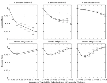
Fig. 5. (a) Impact of the choice of calibration points for interpolator (upper panel) and number of nearest neighbors in parameter search
(lower panel) for Nash-Sutcliffe efficiency likelihood measure. The solid line indicates the mean of the 100 subdivisions (each containing 5000 NOAH-LSM simulations). One standard deviation of variability is indicated by the vertical error bars (dashed).
0.4 0.45 0.5 0.55 0.6 0.65 0.7 0.75 0 0.25 0.5 0.75 1 Success Ratio Nearest Neighbors =6 0 0.25 0.5 0.75 1 Success Ratio Calibration Emin=0.3 0.4 0.45 0.5 0.55 0.6 0.65 0.7 0.75
Acceptance Threshold for Behavioral Sets (>Exponential Efficiency) Nearest Neighbors=12
Calibration Emin=0.5
0.4 0.45 0.5 0.55 0.6 0.65 0.7 0.75 Nearest Neighbors=24
Calibration Emin=0.7
Fig. 5. (b) Same as in (a), but for exponential efficiency likelihood measure.
not necessarily considered a drawback of the interpolator as it can be executed as many times as needed to generate the desired sample size of behavioral parameter sets. The more qualifying aspect is whether the interpolator exhibits regions of local attractions in the response surface that are inconsis-tent with the uniform random sampling (discussed next).
In Figs. 5a and 5b, we explore certain calibration aspects of the interpolator and the N N method for Nash-Sutcliffe and Exponential efficiency likelihood measures, respectively.
The upper panels show the effect of choice of calibration sample points for interpolator for three different criteria (se-lection of points based on a minimum Efficiency value of 0.3, 0.5 and 0.7). The lower panels show the effect of the “n” – the number of nearest neighbors – in interpolating the likelihood value by the N N method for 6, 12 and 24 nearest neighbors. We observe that the choice of calibration points can have an impact on the efficiency (SR value) of the inter-polator with the best performance achieved when the choice
436 F. Hossain et al.: A non-linear and stochastic response surface method −6 −5.5 −5 −4.5 −4 Parameter value 0.4 0.5 0.6 0.7 0.8 0.9 1 Efficiency 0.15 0.25 0.35 0.45 0.4 0.5 0.6 0.7 0.8 0.9 1 Efficiency 2 4 6 8 10 12 14 Parameter value 0.4 0.5 0.6 0.7 0.8 0.9 1 0 0.1 0.2 0.3 0.4 0.5 0.6 0.4 0.5 0.6 0.7 0.8 0.9 1 SMCMAX PSISAT BB Log10 (SATDK)
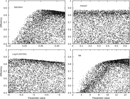
Fig. 6. (a) Dotty plots obtained from uniform random sampling of GLUE model parameters with Nash-Sutcliffe efficiency likelihood measure >0.4. The plots represent an ensemble of 5000 parameter sets.
−6 −5.5 −5 −4.5 −4 Parameter value 0.4 0.5 0.6 0.7 0.8 0.9 1 0.15 0.25 0.35 0.45 0.4 0.5 0.6 0.7 0.8 0.9 1 2 4 6 8 10 12 14 Parameter value 0.4 0.5 0.6 0.7 0.8 0.9 1 0 0.1 0.2 0.3 0.4 0.5 0.6 0.4 0.5 0.6 0.7 0.8 0.9 1 SMCSAT PSISAT Log10 (SATDK) BB
Fig. 6. (b) Same as in (a), but for the interpolator.
of points are highly behavioral (i.e. Emin>0.7). For N N method, the choice of n appears to have a negligible impact, although for both schemes, we observe that the variability in prediction increases as the acceptance criterion increases. Furthermore, the sampling efficiency (in terms of SR) of the
N N method appears to decrease in the moderate likelihood measure ranges (0.2<ENS<0.5; 0.4<EEXP<0.6). We
hy-pothesize that the simple inverse squared distance interpola-tion for N N method is not universally effective for improved
parameter sampling for LSMs because the response surface does not vary isotropically in a linear fashion with respect to parameters.
In Figs. 6a, b and c we compare the dotty plots obtained from the interpolator sampling and the random uniform sam-pling of GLUE model parameters. Dotty plots were first pro-posed by Beven and Binley (1992) as a simple way to demon-strate the parameter equifinality of a model. Against the like-lihood value presented along the y-axis, the scatter of the
pa-0 0.05 0.1 0.15 0.2 Parameter value 0.4 0.5 0.6 0.7 0.8 0.9 1 Efficiency Uniform Sampling 0 0.05 0.1 0.15 0.2 Parameter value 0.4 0.5 0.6 0.7 0.8 0.9 1 Interpolator
Fig. 6. (c) Same as Figs. 6a and 6b, but for the fifth NOAH-LSM parameter of SMCWLT.
rameters along the x-axis is accepted as a qualitative measure of parameter equifinality. If the dotty plots derived from uni-form random sampling are assumed as the reference, then the parameters sampled as behavioral via the initial screening of the interpolator should show similar scatter to represent con-sistent equifinality. This is an important aspect to assess for any parameter sampling scheme, which otherwise may ren-der itself unsuitable for GLUE analysis. The dotty plots for the two likelihood measures were found to be similar. Hence we only show herein dotty plots pertaining to 5000 parameter sets sampled as behavioral for the Nash-Sutcliffe efficiency likelihood measure ENS>0.4. As seen by comparing Fig. 6b
(interpolator dotty plots) with Fig. 6a (uniform random sam-pling) for the four NOAH-LSM parameters, we observe that the behavioral parameters sampled by interpolator represent, at least qualitatively, the same degree of equifinality as the reference (uniform) dotty plots. The fifth parameter compar-ison is shown in Fig. 6c (also found to be similar). The inter-polator has no specific regions of local attraction of uneven sampling inconsistent with the uniform random sampling.
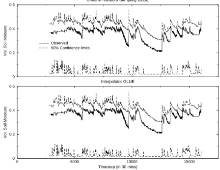
Finally, in Figs. 7a and 7b, we show a typical GLUE anal-ysis with 90% confidence limits in soil moisture simulation uncertainty obtained from the aforementioned 5000 behav-ioral parameter sets – one ensemble sampled by uniform random sampling and the other ensemble sampled via the interpolator. The prediction quantiles produced by uniform random sampling are assumed as the reference for compari-son here. For both likelihood measures (Nash-Sutcliffe ef-ficiency likelihood measure – Fig. 7a lower panel; Expo-nential efficiency likelihood measure – Fig. 7b, lower panel) we observe negligible difference in the uncertainty estima-tion at the 90% confidence limits. However, a more
quali-fying test for the preservation of the uncertainty structure in simulation is provided in Fig. 8 where we compare the Ex-ceedance Probability (EP ) against the width of confidence limits (from 10% to 90%). EP is defined as the number of times the observation (i.e. soil moisture measurement) is not enveloped by the predicted confidence limits normalized by the total number of timesteps in simulation. EP would typ-ically decrease monotontyp-ically with increasing width of the limits. A similarity of the monotonic decrease at high and low widths (>80% and <40%) is observed in Fig. 8. Since GLUE is typically used for uncertainty analyses at high con-fidence limits (Freer et al., 1996; Beven and Freer, 2001) this observation indicates that the interpolator is able to preserve sufficiently accurately the uncertainty structure of soil mois-ture simulation as would have been typically identified with random uniform sampling of the GLUE parameters. How-ever, the use of the current formulation of the interpolator seems most accurate at high confidence limits ranging from 70%–90% for NOAH-LSM soil moisture simulations.
8 Conclusions
This study has presented a simple and efficient scheme for Bayesian assessment of uncertainty in soil moisture simula-tion by a Land Surface Model. The scheme was assessed within a MC simulation framework based on the GLUE methodology. Parameter sampling was improved in the pro-posed scheme by stochastic modeling of the parameter re-sponse surface that recognizes the inherent non-linear deter-ministic behavior of physically complex models. Uncertainty in soil moisture simulation was approximated through a poly-nomial chaos expansion of normal random variables that
rep-438 F. Hossain et al.: A non-linear and stochastic response surface method
0 5000 10000 15000
Timestep (in 30 mins) 0
0.2 0.4 0.6
Vol. Soil Moisture
Interpolator GLUE 0
0.2 0.4 0.6
Vol. Soil Moisture
Uniform Random Sampling GLUE
Observed 90% confidence limits
Fig. 7. (a) The GLUE uncertainty estimation of soil moisture simulation at 90% confidence limits for uniform random sampling (upper
panel) and interpolator (lower panel). Nash-Sutcliffe efficiency likelihood measure >0.4 was used as the acceptance criterion for behavioral parameter sets. Uncertainty estimation for each scenario was conducted from the 5000 sampled sets shown in Figs. 6a, b and c.
0 5000 10000 15000
Timestep (in 30 mins)
0 0.2 0.4 0.6
Vol. Soil Moisture
Interpolator GLUE
0 0.2 0.4 0.6
Vol. Soil Moisture
Uniform Random Sampling GLUE
Observed 90% Confidence limits
Fig. 7. (b) Same as (a), but for Exponential efficiency likelihood measure >0.4 as the acceptance criterion for behavioral parameter sets.
resented the model’s parameter uncertainty. The calibrated polynomial (interpolator) was then used as a fast-running proxy to the slow-running model to predict the degree of rep-resentativeness of a randomly sampled model parameter set. The sampling scheme based on the interpolator was able to reduce computational burden of uniform random MC sam-pling for GLUE by about 10%–70%. It was also found to be 10% more efficient and an order faster than the Nearest-neighborhood sampling method. The GLUE based on the
proposed sampling scheme preserved the uncertainty struc-ture in soil moisstruc-ture simulation at moderate to high confi-dence limits.
Because our proposed interpolator does not impose ad-ditional structural or distributional assumptions on GLUE method that could otherwise compromise its simplicity, it can readily apply to make GLUE parameter sampling for slow-running models more efficient. Some of the natural exten-sions of this work include: (i) application of the interpolator
10 20 30 40 50 60 70 80 90 Width of Confidence Limits (%) 0 0.2 0.4 0.6 0.8 1 Exceedance Probability Nash−Sutcliffe Efficiency
Uniform Random Sampling Interpolator
10 20 30 40 50 60 70 80 90
Width of Confidence Limits (%) Exponential Efficiency
Fig. 8. Response of Exceedance Probability to width of predicted confidence limits. Left panel – Nash-Sutcliffe efficiency likelihood
measure; Right panel – Exponential efficiency measure.
to other physically-complex models and hydrologic variables within the GLUE framework; (ii) investigating the conditions or assumptions that give rise to a chaotic and non-chaotic be-havior in the hydrologic system and thereby attempt to con-nect the relationship of the hydrologic variable to the order of polynomial chaos expansions; and (iii) investigating the effect of the dimensional size of the parameter hyperspace on the sampling efficiency of the interpolator. It has also been suggested that the gradient information of the param-eters with respect to model output, when assimilated in the polynomial chaos expansion, an increase in the prediction accuracy of the interpolator can be expected (Isukapalli and Georgopoulos, 1999). Another potential use of the stochas-tic non-linear response surface sampling scheme would be in applications to large-scale land surface simulations where model parameters are distributed as a matrix (2-D spatial do-main) over large areal scales (>10 000 km2)(note: in this study the parameters were a vector). For such applications, research is needed to explore convenient ways to mathemati-cally reformulate the interpolator to handle such distributed parameters in spatial format. Work is on-going on some of the above aspects and we hope to report them in future.
Acknowledgements. The research associated with this paper was
partially supported by the NASA New Investigator Program (Grant #NAG5-8636). The first author was supported by a NASA Earth System Science Fellowship.
Edited by: B. Sivakumar Reviewed by: two referees
References
Bates, B. C. and Campbell, E. P.: A Markov Chain Monte Carlo scheme for parameter estimation and inference in conceptual rainfall-runoff modeling, Water Resour. Res., 37, 3, 937–947, 2001.
Beck, M. B.: Water Quality Modeling: A Review of the Analysis of Uncertainty, Water Resour. Res., 23, 7, 1393–1442, 1987. Beven, K. J. and Kirkby, M. J.: A physically-based variable
con-tributing area model of basin hydrology. Hydrol. Sci. J., 24, 1, 43–69, 1979.
Beven, K. J. and Freer, J.: Equifinality, data assimilation, and un-certainty estimation in mechanistic modeling of complex envi-ronmental systems using the GLUE methodology, J. of Hydrol., 249, 11–29, 2001.
Beven, K. J. and Binley, A.: The future of distributed models: Model calibration and uncertainty prediction, Hydrol. Proc., 6, 279–298, 1992.
Bras, R. L. and Rodriguez-Rodriguez-Iturbe, I.: Random Functions and Hydrology, Dover Publications, New York, 1993.
Clapp, R. B. and Hornberger, G. M.: Empirical equations for some soil hydraulic properties, Wat. Resour. Res., 14, 601–604, 1978. Collins, D. C. and Avissar, R.: An Evaluation with the Fourier Am-plitude Sensitivity Test (FAST) of which Land Surface Parame-ters are of Greatest Importance in Atmospheric modeling, J. of Climate, 7, 681–703, 1994.
Crawford, T. M., Stensrud, D. J., Mora, F., Merchant, J. W., and Wetzel, P. J.: Value of incorporating satellite-derived land cover data in MM5/PLACE for simulating surface temperatures, J. of Hydrometeorol., 2, 4, 453–468, 2001.
Christaens, K. and Feyen, J.: Constraining soil hydraulic parame-ter and output uncertainty of the distributed hydrological MIKE SHE model using the GLUE framework, Hydrol. Proc., 16, 2, 373, 2002.
Devroye, L.: Non-uniform random variate generation, Springer-Verlag, New York, 1986.
440 F. Hossain et al.: A non-linear and stochastic response surface method
Yongjiu Dai, Zeng, X., Dickinson, R. E., Baker, I., Bonan, G. B., Bosilovich, M. G., Denning, A. S., Dirmeyer, P. A., Houser, P. R., Keith, G. N., Oleson, W., Schlosser, C. A., and Yang, Z.-L.: The Common Land Model. Bull. Amer. Meteorol. Soc, August, 1013–1023, 2003.
Dickinson, R. E., Kennedy, P. J., and Wilson, M. F.: Biosphere Atmosphere Transfer Scheme (BATS) for the NCAR Commu-nity Climate Model, NCAR Tech. Note, NCAR TN275+STR, 69, 1986.
Franks, S. W., Gineste, P., Beven, K. J., and Merot P.: On constrain-ing the predictions of a distributed model: The incorporation of fuzzy estimates of saturated areas into calibration process, Water Resour. Res., 34, 3, 787–797, 1998.
Franks, S. W. and Beven, K. J.: Bayesian estimation of uncertainty in land surface-atmosphere flux predictions, J. of Geophys. Res., 102, D20, 23 991–23 999, 1997.
Freer, J., Beven, K. J., and Ambroise, B.: Bayesian estimation of uncertainty in runoff prediction and the value of data: An appli-cation of the GLUE approach, Water Resour. Res., 32, 6, 2161– 2173, 1996.
Gao, X., Sorooshian, S., and Gupta, H. V.: Sensitivity analysis of the biosphere-atmosphere transfer scheme, J. of Geophys. Res., 101, D3, 7279–7289, 1996.
Ghanem, R. and Spanos, P. D.: Stochastic Finite Elements: A Spec-tral Approach, Springer-Verlag, New York, 1991.
Gutman, G. and Ignatov, G. L.: Derivation of green vegetation frac-tion from NOAA/AVHRR for use in numerical weather predic-tion models, Int. J. Remote Sensing, 19, 7, 1533–1543, 1998. Iman, R. L., Helton, J. C., and Campbell, J. C.: A approach to
sensitivity analysis of Computer Models: Part I – Introduction, Input variable Selection and Preliminary Variable assessment, J. of Qual. Technol. , 13, 3, 174–183, 1981.
Henderson-Sellers, A.: A factorial assessment of sensitivity of the BATs Land-Surface Parameterization Scheme, J. of Climate, 6, 227–247, 1993.
Hossain, F., Anagnostou, E. N., Borga, M., and Dinku, T.: Hydro-logical Model Sensitivity to Parameter and Radar Rainfall Esti-mation Uncertainty. Hydrol. Proc., accepted, 2004.
Isukapalli, S. S. and Georgopolous, P. G.: Computational Meth-ods for Efficient Sensitivity and Uncertainty Analysis of Mod-els for Environmental and Biological Systems (Tech Rep CCL/EDMAS-03, Rutgers University), 1999.
Isukapalli, S. S., Roy A., and Georgopoulos, P. G.: Efficient sen-sitivity/uncertainty analysis using the combined stochastic re-sponse surface method and automated differentiation: Applica-tion to environmental and biological systems, Risk Analysis, 20, 4, 591–602, 2000.
Jayawardena A. W. and Lai, F.: Analysis and prediction of chaos in rainfall and streamflow time series, J. Hydrol., 153, 23–52, 1994.
Kremer, J. N.: Ecological Implications of parameter uncertainty in stochastic simulation, Ecological Modelling, 18, 187–207, 1983. Krzysztofowicz, R.: Hydrologic uncertainty processor for proba-bilistic river stage forecasting, Water Resour. Res., 36, 11, 3265– 3277, 2000.
Kuczera, G. and Parent, E.: Monte Carlo assessment of parame-ter uncertainty in conceptual catchment models: The Metropolis algorithm. J. of Hydrol., 211, 69–85, 1998.
Liu, K.: Soybeans: Chemistry, Technology and Utilization, Chap-man and Hall: New York, 1–22, 1997.
Mahrt, L. and Ek, K.: The Influence of atmospheric stability on potential evaporation, J. Clim. Appl. Meteorol, 23, 1984.
McKay, M. D., Beckman, R. J., and Conover, W. J.: A Comparison of three methods for selecting values of input variables in the analysis of Output from a Computer Codes, Technometrics, 21, 2, 239–245, 1979.
Misirli, F., Gupta, H. V., Sorooshian, S., and Thiemann, M.: Bayesian Recursive estimation of Parameter and Output Un-certainty for watershed models, In Calibration of Watershed Models, edited by Duan, Q. J., Gupta, H. V., Sorooshian, S., Rousseau, A. N., and Turcotte, R., Water Science Application No. 6, AGU: Washington DC, 1125–1132, 2003.
Nash, J. E. and Sutcliffe, J. V.: River Flow forecasting through conceptual models, 1, A discussion of principles, J. Hydrol., 10, 282–290, 1970.
Norman, A. G.: Soybean Physiology, Agronomy, and Utilization, Academic Press: New York, 17–44, 1978.
Pan, H.-L. and Mahrt, L.: Interaction between soil hydrology and boundary layer development, Boundary Layer Meteorol, 38, 185–202, 1987.
Press, W. H., Teukolsky, S. A., Vetterling, W. T., and Flannery, B. P.: Numerical Recipes in Fortran 77 (Second Edition), Cambridge University Press, UK, 1999.
Rodriguez-Iturbe, R. I., Entekhabi, E., Lee, J. S., and Bras, R. L.: Non-linear dynamics of Soil Moisture at Climate Scales, 2. Chaotic Analysis, Water Resour. Res., 27, 7, 1991.
Romanowicz, R. and Beven, K.: Dynamic real-time prediction of flood inundation probabilities, Hydrological Sciences, 43, 2, 181–196, 1998.
Sellers, P. J., Mintz, Y., Sud, Y. C., and Dalcher, A.: A simple bio-sphere model (SiB) for use within general circulation models, J. of Atmos. Sci, 43, 505–531, 1986.
Sivakumar, B.: Chaos theory in hydrology: Important issues and interpretations, J. Hydrol., 227, 1–20, 2000.
Sivakumar, B., Berndtsson, R., Olsson, J., and Jinno, K.: Evidence of chaos in the rainfall-runoff process. Hydrological Sciences, 46, 1, 2001a.
Sivakumar, B., Sorooshian, S., Gupta V. J., and Gao, X.: A chaotic approach to rainfall disaggregation. Water Resour. Res., 37, 1, 61–72, 2001b.
Schulz, K. and Beven, K. J.: Data-supported robust parameteriza-tions in land surface-atmosphere flux predicparameteriza-tions: towards a top-down approach, Hydrol. Proc. 17, 2259–2277, 2003.
Schulz, K., Jarvis, A., and Beven, K.: The predictive uncertainty of land surface fluxes in response to increasing ambient carbon dioxide, J. of Climate, 14, 2551–2562, 2001.
Sridhar, V., Elliot, R. L., Chen F., and Botzge, J. A.: Validation of the NOAH-oSU land surface model using surface flux measure-ments in Oklahoma, J. of Geophys. Res., 107, D20, 2002. Spear, R. C. and Hornberger, G. M.: Eutrophication in Peel Inlet, II,
Identification of critical uncertainties via Generalized Sensitivity Analysis, Wat. Res., 4, 43–49, 1980.
Thiemann, M., Trosset, M., Gupta, H., and Sorooshian, S.: Bayesian recursive parameter estimation for hydrologic models, Water Resour. Res., 37, 10, 2521–2535, 2001.
Tyagi, A. and Haan, C. T.: Uncertainty analysis using first-order approximation method, Water Resour. Res., 37, 5, 1847–1858, 2001.
Young, P. C. and Beven, K. J.: Database mechanistic modeling and rainfall-flow non-linearity, Environmentrics, 5, 3, 335–363, 1994.
Wiener, N.: The Homogeneous Chaos, Amer. J. of Math., 60, 897– 893, 1938.