HAL Id: hal-00302055
https://hal.archives-ouvertes.fr/hal-00302055
Submitted on 1 Jan 2001
HAL is a multi-disciplinary open access
archive for the deposit and dissemination of
sci-entific research documents, whether they are
pub-lished or not. The documents may come from
teaching and research institutions in France or
abroad, or from public or private research centers.
L’archive ouverte pluridisciplinaire HAL, est
destinée au dépôt et à la diffusion de documents
scientifiques de niveau recherche, publiés ou non,
émanant des établissements d’enseignement et de
recherche français ou étrangers, des laboratoires
publics ou privés.
W. A. Nuss, D. K. Miller
To cite this version:
W. A. Nuss, D. K. Miller. Mesoscale predictability under various synoptic regimes. Nonlinear
Pro-cesses in Geophysics, European Geosciences Union (EGU), 2001, 8 (6), pp.429-438. �hal-00302055�
Nonlinear Processes in Geophysics (2001) 8: 429–438
Nonlinear Processes
in Geophysics
c
European Geophysical Society 2001
Mesoscale predictability under various synoptic regimes
W. A. Nuss and D. K. Miller
Department of Meteorology, Code MR/Nu, Naval Postgraduate School, Monterey, CA, USA Received: 18 September 2000 – Revised: 19 March 2001 – Accepted: 9 April 2001
Abstract. Numerical model experiments using slightly ro-tated terrain are compared to gauge the sentivity of mesoscale forecasts to small perturbations that arise due to small synoptic-scale wind direction errors relative to topographic features. The surface and above surface wind speed errors, as well as the precipitation forecast errors, are examined for a landfalling cold front that occurred during the Cali-fornia Landfalling Jets (CALJET) experiment. The slight rotation in the terrain results in nearly identical synoptic-scale forecasts, but result in substantial forecast errors on the mesoscale in both wind and precipitation. The largest mesoscale errors occur when the front interacts with the to-pography, which feeds back on the frontal dynamics to pro-duce differing frontal structures, which, in turn, result in mesoscale errors as large as 40% (60%) of the observed mesoscale variability in rainfall (winds). This sensitivity dif-fers for the two rotations and a simple average can still have a substantial error. The magnitude of these errors is very large given the size of the perturbation, which raises concerns about the predictability of the detailed mesoscale structure for landfalling fronts.
1 Introduction and motivation
The capability to run mesoscale models is now widespread and forecasts on very small-scales are being routinely gen-erated by many groups. Previous studies by Anthes (1986), Baumhefner (1984), and others have focused on the growth of synoptic-scale errors and their impact on predictabil-ity. Results from Baumhefner (1984) indicate that the typ-ical error doubling time is about 2 days for the synop-tic scale and that it may decrease with decreasing synopsynop-tic scale. Tennekes (1978) suggests that the mesoscale rapid growth of errors will occur due to the transfer of energy from smaller scales to larger scales by three-dimensional turbulence, which will further decrease the predictability Correspondence to: W. A. Nuss ([email protected])
time limit. However, for mesoscale phenomena that do not fit the average spectrum of turbulence, this rate of energy transfer and thus, the forecast error may be quite differ-ent. Warner (1992) suggests that some mesoscale phenom-ena may be more predictable than others, especially those forced by strong fixed surface features such as the mesoscale terrain. This assertion has not been widely tested and many efforts in mesoscale numerical forecasting are based upon this unproven assertion. This assertion is examined for one event in order to investigate the impact of small synoptic-scale errors on the mesosynoptic-scale error growth.
To further complicate the practical problem, many of the fine scale resolution forecasts are generated from ei-ther larger-scale numerical model analyses and forecasts, or occasionally from reanalysis of synoptic-scale analyses, using coarse resolution observational networks. The im-pact of coarse resolution initial conditions on the quality of mesoscale forecasts may also contribute to the fundamental predictability limits on the mesoscale. The overall goal of our study is to examine the impact of small-synoptic scale variations on the growth of mesoscale error.
The relationship between mesoscale error growth and the variability of synoptic-scale structures used to initiate those forecasts is not well-known, but has significant implications for the application of those forecasts. Kuypers (2000) ex-amined the growth of error on the 4 km nest of a mesoscale model initiated with ten slightly different synoptic-scale ini-tial states and found that the growth can be quite rapid, and surface wind speed errors in excess of 8 m/s were reached within 18 h for a landfalling cold front. Key questions that motivate this study are: how do small variations in synoptic analyses impact mesoscale forecast errors; and how correct must the synoptic scale be in order to limit mesoscale error growth? Rapid and large growth of the mesoscale forecast error within 24 h may essentially render the mesoscale fore-cast unskillful, which might indicate that the predictability limit has been exceeded. This study examines these issues for one of several cases of mesoscale forecasts of weather events along the California coast.
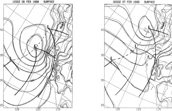
Fig. 1. Comparison of the synoptic-scale sea-level pressure forecasts for three numerical model experiments, using slightly rotated
topogra-phy. The (a) 12-h and (b) 24-h forecasts are overlaid for all three forecasts. The approximate positions of the surface low, and the warm and cold fronts for the initial time, 12-h and 24-h forecasts are shown in both (a) and (b).
25 30 35 40 45 50 55 60 -145 -140 -135 -130 -125 -120 -115 -110 25 30 35 40 45 50 55 60 -145 -140 -135 -130 -125 -120 -115 -110 25 30 35 40 45 50 55 60 -145 -140 -135 -130 -125 -120 -115 -110 25 30 35 40 45 50 55 60 -145 -140 -135 -130 -125 -120 -115 -110
Fig. 2. The four model domains used to conduct the numerical
sim-ulations. The grid spacing for the outer nest is 108 km, the second nest is 36 km, the third nest is 12 km, and the fourth nest is 4 km. Part of the rectangular outer nest is not shown due to the orientation of the plot.
2 Synoptic situation and experiment design
The meteorological situation that has been studied is associ-ated with a landfalling cyclone and front along the U.S. west coast. The case occurred on 5–6 February 1998 during the California Landfalling Jets (CALJET) experiment and its
ba-Fig. 3. The orientation of the coastline for the coarsest domain
(108 km nest) for the three experiments. The relative shift in the coastline represents the relative rotation of the topography for the experiments.
sic evolution is depicted in Fig. 1. A low pressure center de-veloped along the trailing front from a previous cyclone and underwent cyclogenesis as it tracked northeastward just off the California coast. As the cyclone tracked northeastward, the trailing cold front passed through the central California region between 14:00 and 21:00 UTC on 6 February, as
sug-W. A. Nuss and D. K. Miller: Mesoscale predictability under various synoptic regimes 431
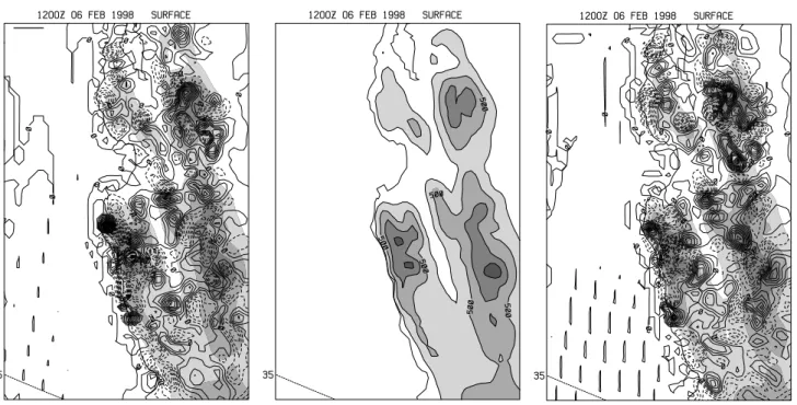
Fig. 4. (a) Difference in terrain elevations between Exp. 3 and the control, plotted in meters with a 10 m contour interval, overlaid on the
control topography, and shaded at 250 m intervals. (b) Unrotated topography (control) plotted in meters with a 250 m contour shaded interval.
(c) Difference in terrain elevations between Exp. 2 and the control, plotted in meters with a 10 m contour interval, overlaid on the control
topography, and shaded at 250 m intervals.
gested by the frontal analysis depicted in Fig. 1. The front passes through the 4 km nest of the model in a north-south orientation.
The basic model configuration is depicted in Fig. 2, which shows a four domain setup that varies from 108 km grid spac-ing on the coarsest nest to 4 km spacspac-ing on the fine nest. The NCAR/Penn State MM5 model (Grell et al., 1994) was used to conduct these experiments and was run with 30 vertical levels. The MRF boundary layer parameterization and Kain-Fritsch cumulus parameterization on the outer 3 nests, with explicit cloud physics on the 4 km nest, were used. The ini-tial analyses were constructed from the U.S. Navy’s global forecast model (NOGAPS), using two-dimensional, multi-quadric interpolation (Nuss and Titley, 1994) at the standard pressure levels. NOGAPS forecasts were used to supply the lateral boundary conditions on the outer nest. Given that the structure on the mesoscale domains was determined from the NOGAPS model, which contains no mesoscale structure, the model had to internally spin-up its own mesoscale structure. Three experiments were conducted for this study to exam-ine the sensitivity of the mesoscale forecasts to slight differ-ences in the synoptic-scale flow. The experiments consisted of a control simulation and two experiments where the ter-rain was rotated by approximately plus or minus one degree relative to the center of the mesoscale domain. Experiment 2 consists of a one degree clockwise rotation of the topography around the center on the 4 km nest. Experiment 3 consisted of a one degree counterclockwise rotation around the same point. These rotations result in the incoming flow, with the front slightly more or less perpendicular to the coastal
topog-raphy. Figure 3 compares the differences on the coastline in the 108 km grid for the three experiments and shows that the differences, even at coarse resolution, are very small. Note that although the topography has been rotated, the dynamic and thermodynamic structure is unaltered, and the grid points occur at the same latitude and longitude in all experiments. This results in the same meteorological forcing that interacts with a slightly different projection of the topography onto the flow for the three experiments. Figure 4 compares the topog-raphy for the 4 km nest. The center panel (Fig. 4b) depicts the terrain for the control experiment and the left (Fig. 4a) and right (Fig. 4c) panels show the difference between this terrain and that of Exp. 3 (left) and Exp. 2 (right). The differ-ences occur due to the slightly different locations of the peaks and valleys, compared to the unrotated topography. The re-sult is a nearly random distribution of differences, with a root mean squared (RMS) deviation of around 18 m for both ex-periments.
Figure 1 also compares the evolution of sea-level pressure on the 36 km grid to show that the synoptic-scale evolution is nearly identical in the three experiments. The mean sea-level pressure differs by less than 0.5 hPa in the regions with the largest deviation and is much smaller over most of the do-main. More importantly, the structure of the pressure field is nearly identical, with the cyclone center and the front in es-sentially the same locations at this coarsest scale. The small magnitude of the differences in the synoptic-scale structure seen in the sea-level pressure field is representative of the er-rors throughout the model atmosphere for all variables. This indicates the strong similarity in the evolution of the larger
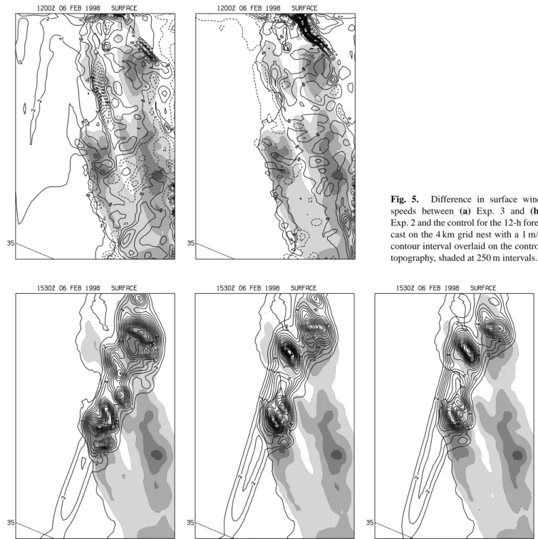
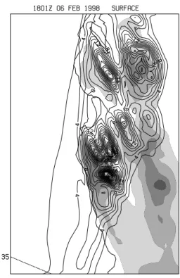
Fig. 5. Difference in surface wind speeds between (a) Exp. 3 and (b) Exp. 2 and the control for the 12-h fore-cast on the 4 km grid nest with a 1 m/s contour interval overlaid on the control topography, shaded at 250 m intervals.
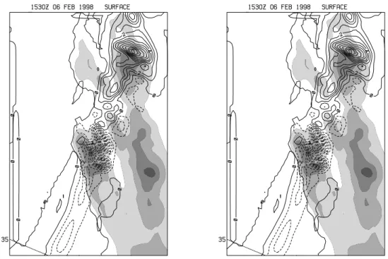
Fig. 6. One hour accumulated precipitation ending at the 15:30 UTC forecast time for (a) Exp. 3, (b) control, and (c) Exp. 2. The one hour
precipitation is contoured every 1 mm, overlaid on the control topography, and shaded at 250 m intervals.
scale structure of the model atmosphere.
3 Character of mesoscale errors
In order to begin to characterize the mesoscale forecast error due to the slight difference in topography, the differences in near surface wind speeds were calculated between the two experiments and the control. A representative sample of these differences for the 12 h forecast is shown in Fig. 5 and
is summarized in Table 1 by the root mean squared (RMS) deviations between Exps. 2 and 3, and the control at 6 h inter-vals in the forecast. For purposes of this paper, the RMS de-viation between the rotated terrain experiments and the con-trol with no terrain rotation, will be referred to as an error. Although this is not strictly an error relative to a true atmo-spheric structure, it represents a departure due to a small per-turbation, and the growth of this departure could contribute to actual error growth when compared to a known true struc-ture. This sensitivity to small perturbations is the main focus
W. A. Nuss and D. K. Miller: Mesoscale predictability under various synoptic regimes 433
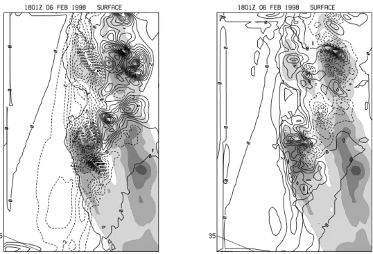
Fig. 7. Difference (Exps. minus control) in one hour precipitation accumulations between the control and Exps. (a) 3 and (b) 2, where the
frontal timing differences are not taken into account. Contours are every 1 mm, with negative differences shown as dashed lines, overlaid on the control topography, and shaded at 250 m intervals.
Fig. 8. Same as Fig. 7, except that the differences in frontal timing are taken into account.
of this study and will be treated as an error.
The first thing to note about the distribution of surface wind speed errors (Fig. 5) is that they are large near the to-pography and very small over the ocean part of the domain. Maximum deviations are as large as 15 m/s, with the maxi-mum surface winds around 25 m/s, although the largest error and largest wind speeds are not necessarily coincident. The
regions with the largest error tend to occur in the lee of the topography, although this is not always the case. A compar-ison between the Exps. 3 and 2 differences show that the er-rors often have the opposite sign, although this is not always true, and the magnitude of the errors can differ substantially. The differing error characteristics arise from slightly differ-ent flow interactions with the model topography, which is
Fig. 9. Four hour accumulated precipitation from the control
exper-iment as the front passes through the domain. Contours are every 2 mm, overlaid on the control topography, and shaded at 250 m in-tervals.
not symmetric. This implies that simple ensemble averaging would not eliminate these types of errors.
Table 1. Root Mean Squared (RMS) surface wind speed
differ-ence/error (Exp. - control) for Exp. 3 (column 1) and Exp. 2 (col-umn 2) at 6 hour intervals through the forecast. Errors are for the 4 km model nest Exp 3 Exp 2 F00 0.22 m/s 0.21 m/s F06 1.03 m/s 1.07 m/s F12 1.40 m/s 1.18 m/s F18 2.52 m/s 1.40 m/s F24 1.81 m/s 0.87 m/s
The growth of mesoscale error over time, given in Table 1, does not exhibit classic predictability error growth. This is primarily due to the presense of the front in the domain and the generation of mesoscale structure due to its interaction with the terrain. Note that the RMS wind error at the ini-tial time (F00) is due to the slightly different locations of the grid points relative to the control (unrotated) topography, which is used as the reference grid for comparison. This er-ror would be zero if a direct grid point-to-grid point compar-ison is made, but all errors were calculated by first rotating the forecasts back to the reference topography of the control. Both Exps. 2 and 3 show rapid growth of the RMS error
dur-ing the first 6 h of the forecast to just over 1.0 m/s. Although this is not a huge error, it arises from maximum absolute er-rors as large as 15 m/s. The error grows substantially during the next 12 h, especially for Exp. 3, and then drops by the 24-h forecast. T24-his be24-haviour can be attributed to t24-he passage of the front through the 4 km nest between the 6- and 24-h fore-casts when the front is primarily outside of this nest. This behaviour is mirrored above the surface as well to produce the largest differences at any given model level during the time that the front is within the 4 km nest. The comparison of the RMS error between the two experiments at a given fore-cast time does, however, reflect real differences in the error between the two experiments, with Exp. 3 having a substan-tially larger error than Exp. 2 for most time periods.
The model predicted precipitation accumulation over 1 h shows that there are both timing differences in the frontal passage (phase error) and small-scale precipitation distribu-tion differences (structure error). Figure 6 depicts the 1 h precipitation accumulations for the 15:30 UTC forecast time for the three experiments as the front crosses the coast near Monterey. The figure shows that the front moves faster (by about 45 min) in Exp. 3 and slower (by 15 min) in Exp. 2, compared to the control. These timing differences give rise to differences in precipitation simply due to the fact that the front is interacting with different parts of the coastal moun-tains in the three experiments at any given forecast time. For example, Exp. 3 shows the heaviest precipitation just east of the southern San Francisco (SF) Bay region, while the control and Exp. 2 put the maximum just east of the Santa Cruz Mountains, just south of the SF Bay. These differ-ences are highlighted in Figs. 7 and 8, which show the dif-ferences in 1 h precipitation, either correcting for the phase differences (Fig. 8) or not correcting for the phase differences (Fig. 7). The uncorrected differences in Fig. 7 show strong positive/negative couplets in the differences centered on the frontal location, which is highly indicative of the phase error. The RMS error for the uncorrected forecasts is 3.9 mm and 1.6 mm for Exps. 3 and 2, respectively. These RMS differ-ences compare to an average 1 h precipitation of 3.6 mm and 4.3 mm over the domain for experiments 2 and 3, respec-tively, each with a standard deviation around the mean of 2.5 mm. These indicate that Exp. 3 has a relatively large er-ror when normalized by the mean precipitation, which seems to largely be due to the phase error. However, when the tim-ing of the frontal passage is taken into account (Fig. 8), the errors for both Exps. 2 and 3 are less (1.21 and 2.81 mm, re-spectively). The plotted difference field shown in Fig. 8 now highlights the mesoscale structure error not due to the phase error. In this case, Exp. 3 can be seen as significantly worse, with a maximum difference of more than 12 mm in an hour. The figure also shows that the precipitation has a rather dif-ferent distribution with higher rainfall to the north and east, and lower rainfall along the coast to the south, compared to the control. These differences cannot be simply explained by the one degree rotation of the coastal topography and must represent dynamic feedback between the topography and the precipitating front.
W. A. Nuss and D. K. Miller: Mesoscale predictability under various synoptic regimes 435
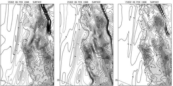
Fig. 10. Difference (Exps. minus control) in four hour accumulated precipitation for (a) Exp. 3 and (b) Exp. 2, where the difference in timing
of the frontal passages has been taken into account. Contours are every 1 mm with negative values (control higher) shown as dashed lines, overlaid on the control topography, and shaded at 250 m intervals.
Fig. 11. Difference between Exp. 2 plus 3 average four hour
ac-cumulated precipitation and the control. Contours are every 1 mm with negative values (control higher) shown as dashed lines, over-laid on the control topography, and shaded at 250 m intervals.
Since these differences in 1-h precipitation might be due to short-term effects, the 4-h accumulated precipitation over the time period when the front crosses the mesoscale nest (storm total) was also compared. The control distribution is shown in Fig. 9 where the maximum rainfall amounts are ob-served near the highest topography, and the amounts range from 10 to greater than 20 mm for the 4-h storm total pre-cipitation. The difference in the 4-h accumulated precipita-tion after the adjustment for timing differences is shown in Figs. 10a (Exp. 3) and 10b (Exp. 2). These figures show that the accumulated precipitation error can be as large as the precipitation accumulations in the control and that there is a distinct difference between the two experiments. Exp. 3 pro-duces more rainfall along the inland ranges, while Exp. 2 is higher along the coast than the control. Since Exp. 3 is as-sociated with a more direct onshore flow than Exp. 2, these differences do not appear to be due to the simple process that is associated with the flow being more perpendicular to the mountains. If this were the case, Exp. 3 would tend to have higher precipitation along the coastal mountains, which are oriented slightly more transverse to the flow than in the con-trol. These precipitation differences between the two experi-ments represent the impact of the differing flow interactions with the complex topography, and do not cancel each other out by ensemble averaging. This is illustrated in Fig. 11, which shows a simple average of the two forecasts (two-member ensemble) and its associated error. While the RMS error is smaller than either Exps. 2 or 3, the error can still be quite large in some locations.
Fig. 12. Difference (Exp. minus control) in surface wind speeds between (a) Exp. 3, (b) 36 km control forecast, and (c) Exp. 2 and the
control for the 15:30 UTC forecast time on the 4 km grid nest. Contour interval is every 1 m/s with negative values (control higher) shown as dashed lines, overlaid on the control topography, and shaded at 250 m intervals.
Fig. 13. Difference (Exp. minus
con-trol) in wind speeds at 800 hPa between
(a) Exp. 3 and (b) Exp. 2 and the control
for the 15:30 UTC forecast time on the 4 km grid nest. Contour interval is ev-ery 1 m/s with negative values (control higher) shown as dashed lines, overlaid on the control topography, and shaded at 250 m intervals.
The surface wind speed errors at the time that the front is interacting with the topography are illustrated in Fig. 12. As noted above for the earlier time period, the surface wind speed differences are largest near the topographic features and these errors are not completely symmetric in the two ferent rotations. The figure also shows that wind speed dif-ferences also occur along the front, particularly for Exp. 3. The uncorrected RMS wind errors are 2.72 m/s and 1.51 m/s for Exps. 3 and 2, compared to a 3.03 m/s standard deviation
about the mean for the control forecast. Correcting for the timing of the frontal passage reduces these errors to 1.86 and 1.22 m/s for Exps. 3 and 2, respectively. One measure of pre-dictive skill is whether the forecast RMS error exceeds the natural variability of the mesoscale atmosphere, as reflected by the standard deviation about the mean. If it does, then simply using the mean value over the entire forecast domain would have a lower RMS error than the mesoscale forecast it-self (no skill). Another measure of predictive skill is whether
W. A. Nuss and D. K. Miller: Mesoscale predictability under various synoptic regimes 437
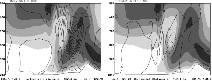
Fig. 14. Cross section across the front of the along-front wind speed (shaded) every 4 m/s and the difference (Control minus Exp. 3, left, and
Control minus Exp. 2, right) in the along-front wind speeds (heavy lines) every 2 m/s. Negative differences (Exps. are higher) are shown as dashed lines. Position of the surface cold front is approximately at the center of the cross section.
a synoptic-scale forecast shows larger or smaller errors com-pared to a mesoscale forecast. If the errors are smaller for the synoptic-scale forecast, then again, the mesoscale forecast exhibits no skill compared to the synoptic scale forecast. Fig-ure 12b illustrates the error that occurs if the forecast on the 36 km grid is taken to be the mesoscale wind forecast on the 4 km grid. In this case, the wind errors follow the topogra-phy even more strongly as the 36 km forecast fails to resolve the smaller scale topographic features. The RMS error for the synoptic-scale forecast is 3.10 m/s, only slightly worse than Exp. 3 (uncorrected). This shows that the mesoscale forecasts have some relative skill compared to both the mean surface winds over the domain and the 36 km synoptic-scale forecast, although the skill may be rather small at times.
Table 2. Root Mean Squared (RMS) wind speed difference/error at
800 hPa (Exp. - control) for Exp. 3 (column 1) and Exp. 2 (column 2) at 6-h intervals through the forecast. Errors are for the 4 km model nest Exp 3 Exp 2 F00 0.16 m/s 0.14 m/s F06 0.75 m/s 0.56 m/s F12 1.75 m/s 0.58 m/s F18 3.09 m/s 1.56 m/s F24 1.48 m/s 1.26 m/s
The surface wind errors are largest near the topography, but they also seem to indicate differences in the frontal forc-ing as well. To characterize the wind errors just above the topography, the RMS error at the 800 hPa level was exam-ined. Figure 13 shows the distribution of this error for the 15:30 UTC forecast time for the two experiments. From this plot, it is evident that most of the differences are due solely to
flow differences around the front itself, with only small errors elsewhere. Evidently, the difference in topographic orienta-tion has allowed the front to evolve rather differently in the two experiments. The exact cause for these differing frontal evolutions is not known at this time, but clearly the error in the atmosphere above the topography is due to this dynamic feedback. The comparison of RMS wind speed errors over time, shown in Table 2, also highlights the large jump in the RMS error when the front is in the 4 km domain for the F12 and F18 time periods. The difference in the RMS error for the two experiments at F12 is due primarily to the phase dif-ference between them, where the front has yet to interact with the topography in Exp. 2, but is already interacting in Exp. 3. Phase shifting has less impact on the RMS error at this level, since the phase corrected RMS error is 2.71 and 1.69 m/s for Exps. 3 and 2, respectively, compared to 2.93 and 1.65 m/s when the phase error is not taken into account. The lack of error reduction due to correcting for the phase error is ev-idently due to small-scale frontal structure differences that are not due to any phase shift.
The frontal differences become even more evident on a cross section through the front at the 15:30 UTC forecast time. The phase corrected wind speed difference is shown in Fig. 14, which indicates flow differences around the front, particularly above the surface. Experiment 3 (Fig. 14a) has a weaker pre-frontal jet, with the largest difference around 800 hPa. Experiment 2 (Fig. 14b) has a slightly stronger pre-frontal jet at about the same level. These differences are con-sistent with the flow being more perpendicular to the topog-raphy in Exp. 3 (slower jet) and more parallel in Exp. 2 (faster jet), although the jet occurs above the topography. The dif-ferences also seem to be rather large given only a one degree rotation of the topography.
4 Conclusions
The comparison of the MM5 model forecasts, using a slightly rotated topography, show substantial sensitivity of the mesoscale wind and precipitation predictions to this per-turbation of the flow. For this landfalling front, the mesoscale RMS errors in surface winds were as large as 40–60% of the observed variability in the surface winds over the mesoscale domain, and storm total precipitation accumulation errors were 20–40% of the observed variability. These errors were strongly tied to the primary terrain features, but arose due to differing flow interactions with the terrain in the various simulations. The flow direction relative to the topography resulted in different frontal structures. The mesoscale errors grew rapidly (within 6 h of the model start time) and substan-tially increased as the front entered the mesoscale (4 km) do-main and interacted with the topography. The errors above the surface were strongly tied to the front and its differ-ing structure between the three experiments. The fact that the initial synoptic-scale differences were very small (one degree rotation of the terrain) and that the mesoscale error grew rapidly indicates that in some situations, a nearly per-fect synoptic-scale analysis and forecast may be insufficient to obtain the mesoscale details in the wind and a correct precipitation measurement. Although this is a single case, this model sensitivity suggests that the predictability of the mesoscale structure may be very limited for some landfalling fronts. The general application of this result to other
land-falling fronts is not known and is presently under investiga-tion.
References
Anthes, R. A.: The general question of predictability, in: Mesoscale Meteorology and Forecasting, (Ed) Ray, P. S., Amer. Meteor. Soc., 636–655, 1986.
Baumhefner, D. P.: The relationship between present large-scale forecast skill and new estimates of predictability error growth, in: Predictability of Fluid Motions (La Jolla Institute- 1983),(Eds) Holloway, G. and West, B. J., American Institute of Physics, New York, 169–180, 1984.
Grell, G. A., Dudhia, J., and Stauffer, D. R.: A description of the fifth-generation Penn State/NCAR Mesoscale Model (MM5), NCAR Tech. Note NCAR/TN-398+STR, (Available from the National Center for Atmospheric Research, P.O. Box 3000, Boulder, CO 80307.), pp. 138, 1994.
Kuypers, M. A.: Understanding mesoscale error growth and pre-dictability, M.S. Thesis, Naval Postgraduate School, Monterey, CA 93943, pp. 114, 2000.
Nuss, W. A. and Titley, D. W.: Use of multiquadric interpolation for meteorological objective analysis, Mon. Wea. Rev., 122, 1611– 1631, 1994.
Tennekes, H.: Turbulent flow in two and three dimensions, Bull. Amer. Met. Soc., 59, 22–28, 1978.
Warner, T. T.: Modeling of surface efects on the mesoscale, in: Mesoscale Modeling of the Atmosphere, (Eds) Pielke, R. A. and Pearce, R. P., Amer. Meteor. Soc., 21–27, 1992.