HAL Id: hal-00304836
https://hal.archives-ouvertes.fr/hal-00304836
Submitted on 4 Apr 2006
HAL is a multi-disciplinary open access
archive for the deposit and dissemination of
sci-entific research documents, whether they are
pub-lished or not. The documents may come from
teaching and research institutions in France or
abroad, or from public or private research centers.
L’archive ouverte pluridisciplinaire HAL, est
destinée au dépôt et à la diffusion de documents
scientifiques de niveau recherche, publiés ou non,
émanant des établissements d’enseignement et de
recherche français ou étrangers, des laboratoires
publics ou privés.
B. Ahrens
To cite this version:
B. Ahrens. Distance in spatial interpolation of daily rain gauge data. Hydrology and Earth System
Sciences Discussions, European Geosciences Union, 2006, 10 (2), pp.197-208. �hal-00304836�
under a Creative Commons License.
Sciences
Distance in spatial interpolation of daily rain gauge data
B. Ahrens1,*1Institut f¨ur Meteorologie und Geophysik, Universit¨at Wien, Austria
*now at: Institute for Atmosphere and Climate, ETH Zurich, Switzerland
Received: 10 August 2005 – Published in Hydrol. Earth Syst. Sci. Discuss.: 8 September 2005 Revised: 29 November 2005 – Accepted: 7 February 2006 – Published: 4 April 2006
Abstract. Spatial interpolation of rain gauge data is
impor-tant in forcing of hydrological simulations or evaluation of weather predictions, for example. This paper investigates the application of statistical distance, like one minus com-mon variance of observation time series, between data sites instead of geographical distance in interpolation. Here, as a typical representative of interpolation methods the inverse distance weighting interpolation is applied and the test data is daily precipitation observed in Austria. Choosing statis-tical distance instead of geographical distance in interpola-tion of available coarse network observainterpola-tions to sites of a denser network, which is not reporting for the interpolation date, yields more robust interpolation results. The most dis-tinct performance enhancement is in or close to mountainous terrain. Therefore, application of statistical distance in the inverse distance weighting interpolation or in similar meth-ods can parsimoniously densify the currently available obser-vation network. Additionally, the success further motivates search for conceptual rain–orography interaction models as components of spatial rain interpolation algorithms in moun-tainous terrain.
1 Introduction
Precipitation maps with daily or better resolution are neces-sary for investigation of the climatology of extreme events (e.g. Skoda et al., 2003; Palecki et al., 2005), as input in hydrological modeling (e.g. Singh and Frevert, 2002a,b), or in evaluation of numerical weather prediction models (e.g. Beck et al., 2004), for example. Depending on application the maps have to be available close to real–time (e.g. in de-tection of flood generating processes) or it is possible to wait Correspondence to: B. Ahrens
some time and gather as much rain observation data as pos-sible (e.g. in climatology).
The back-bone of these maps are rain gauge data since the reliability of remote sensing data (e.g., by weather radar or satellite) is not high enough (e.g., Young et al., 1999;
Ciach et al., 2000; Adler et al., 2001). A challenge in
mapping is the temporal variation of spatial coverage of available rain gauges. For example, the monthly monitor-ing product of the Global Precipitation Climatology Centre (http://gpcc.dwd.de) is based on about 6000 stations avail-able in near real-time. A second product, the so-called full product, is based on 40 000 stations in the late 1980s but based on only about 20 000 stations in the year 2000. An-other example of time-delay in data availability is a daily precipitation atlas by Rubel (1996) with gridspacing of a few tens of kilometers for the Baltic sea and its drainage basin
(area: 1.7e6 km2). Rubel (1996) is based on about 400
sta-tions and its update by Rubel and Hantel (2001) is based on a 10-times denser station network. Liebmann and Allured (2005) gives a very recent example of varying observation network density in precipitation mapping.
The essence of precipitation mapping is the interpolation
of point data (the rain gauge orifices of ∼1000 cm2are small
compared to the mapping scale, thus the observation sites are considered to be points in good approximation) and spatial averaging or smoothing of the interpolated point data. This leads to precipitation fields with spatial gridspacing and cell support of, for example, a few tens of kilometers. Mapping of rain gauge data is a point-to-area interpolation of the avail-able information.
Auer et al. (2005) developed a homogenized data set of long series of monthly precipitation at 192 station sites in the European Alps and their surroundings. Relative series homogenization relies on significant common variability be-tween neighbored site series assumed to be expressible as
common variance R2 with R the linear correlation
0
1000
2000
3000
4000
0.0
0.2
0.4
elevation [mMSL]
rel. frequency
orography
all stations
50 stations
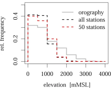
Fig. 1. Height distributions of the Austrian orography, of all
consid-ered rain gauges, and of a subset of 50 gauges on an approximately regular spatial grid.
Scheifinger et al. (2003) estimated that on average a net-work density of about 1/100 km is necessary for establishing
R2≥0.5 in the greater Alpine region, and the average site–
to–site distance increases backwards in time from 61 km in the second half of the 20th century to 74 km in the late 19th century and up to about 200 km in the early 19th century. Thus relative homogenization is not possible in the early 19th century. Relative series homogenization is a point-to-point transformation or interpolation of information.
Another, closely related point-to-point interpolation chal-lenge is estimation of missing data, i.e. filling in the precip-itation time series of a temporarily not reporting station by using information of neighboring stations. Methods for fill-ing in are, for example, inverse distance weightfill-ing (IDW) interpolation, ordinary Kriging, or multiple linear regression using the least absolute deviations criterium (Eischeid et al., 2000). These authors concluded that in interpolation of daily precipitation data “the preselection of surrounding stations, based on their relationship with the station to be estimated, is an integral first step” of all interpolation methods, but with least absolute regression outperforming the other methods in their application.
The relationship between stations is considered differently in the mentioned interpolation methods. The standard IDW method expresses relationship in terms of geographical dis-tance; the Kriging variants apply variogram models which are in typical implementations monotonic functions of geo-graphical distance; and multiple regression applies some sta-tistical distance between the observation time series. There-fore, Tobler’s first law of geography (Tobler, 1970) that all things are related, but nearby things are more related than distant things, is respected in all methods, but with different interpretations of distance.
This paper discusses application of different statistical dis-tances instead of geographical distance in interpolation of ob-servations of a coarse station network to station sites that are not reporting at the interpolation date. Therefore, it discusses the filling in challenge. But, here the challenge is filling in hundreds of observations of a fine-grid station network from an available coarse-grid network with varying network den-sity. The data sets, here from Austria, will be introduced in the next section. The goal is to test a parsimonious method for effective network densification that has the potential to improve rainfall mapping. Section 3 explains how to use some statistical distance measure instead of geographical dis-tance in the often applied, easily to comprehend and imple-ment IDW method. Section 3 explains why IDW is an ideal vehicle for illustrating the advantages and disadvantages of statistical distance and interpolation results will be shown in Sect. 4. Finally, some conclusions and a brief outlook are given.
2 Data
For evaluation of precipitation interpolation methods assum-ing different mean observassum-ing station distances a dense refer-ence network of precipitation stations is necessary. In this investigation a data set of about 900 stations with long daily time series (in the period 1971 to 2002) has been available
for Austria (total area is 84 000 km2) as provided by the
Hy-drographisches Zentralb¨uro, Vienna (delivery date: February 2005). Austria is a country with 62% covered by the Aus-trian Alps and only 32% below 500 m, cf. Fig. 1, and thus interpolation is done in complex mountainous terrain.
The chosen year for the interpolation experiments is 1999. All stations with missing data in 1999 and not at least twenty years of data are erased from the data set and the investi-gations are done with the remaining 710 station time series. This set of stations is named ALL in the following.
In this set of ALL stations the mean next station inter– distance is 6.7 km, but the stations are not regularly dis-tributed within the domain of investigation. They are clus-tered around Vienna in the north-east of the domain and in the main Alpine valley floors (Fig. 2). The irregularity is also illustrated in Fig. 1 which compares the orographic height distribution with distributions of station heights. The lower altitudes are relatively better represented by stations than higher elevations.
In the interpolation experiments this paper applies subsets of ALL stations with 25, 50, and 150 members as observing stations and subsets of the remaining stations with 300 mem-bers as evaluating stations, which are considered in the in-terpolation experiments as temporarily not reporting station but with a long time series of data. The subsets are drawn in a fashion that approximately maximizes the next station geographic inter-distance. One station of the minimum dis-tance pair is erased until the wished number of observing and
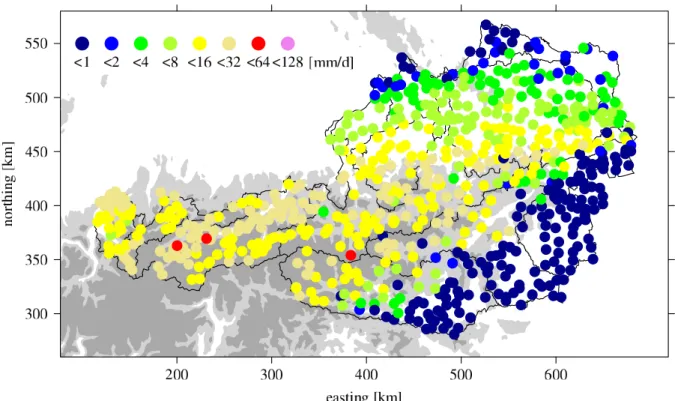
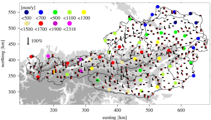
Fig. 2. Rain gauges locations of set ALL (bullets) considered in the present investigation and measured values (bullet colors) for 19 August
1999. The orography is indicated by grey shading (light-grey: elevations above 800 m m.s.l., and dark-grey: elevations above 1500 m m.s.l.). The main Austrian watersheds are indicated by black isolines.
subsequently of evaluating stations is left. Table 1 gives min-imum, mean, and maximum geographic distance and next
neighbor common variance R2. The mean R2increases with
number of stations as expected and consequently the mean interpolation performance should increase. It is noteworthy that for all station sets there are sites which are statistically
far from all the others, i.e. R2<0.5. The number of 150
sta-tions is chosen since this is about the number of stasta-tions that are operational at the Austrian national weather service. This is a globally comparably dense operational network. But, the data of the weather service is not used here since different data sets with different measurement device types and qual-ity control shall be avoided here for the sake of simplicqual-ity.
The chosen regularizing sub-sampling leads to decluster-ing of the considered station sets, but as Fig. 1 illustrates the elevation distribution of the stations is only slightly im-proved. It should be kept in mind that typical station net-works are clustered and thus the effective number of stations in mapping is smaller than the nominal number of stations. Random sub-sampling experiments lead to decreasing inter-polation performance, but this will not be discussed further.
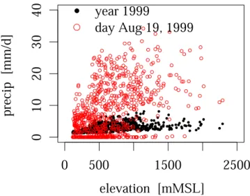
In climatological mapping of precipitation in mountainous terrain a precipitation-elevation relationship is often success-fully considered (cf. Sevruk, 1997). This elevation depen-dence is illustrated in Fig. 3 for yearly data. It is also illus-trated that such a dependence is less obvious at shorter time scales because of the large scatter of the daily precipitation
Table 1. Statistics of the geographic distances of the considered
station sets and statistics of the common variance R2of daily
pre-cipitation series.
set distance [km] R2[%]
min mean max min mean max
ALL/710 1 7 21 40 73 97
25 43 54 69 28 41 53
50 29 36 53 29 50 69
150 16 20 37 41 61 77
values. This will be discussed in some more detail in the following section.
3 Interpolation method
For illustrational purposes the Inverse Distance Weighting in-terpolation (IDW) method is applied. IDW assigns weights to neighboring observed values based on distance to the inter-polation location and the interpolated value is the weighted average of the observations. IDW is applied in many precip-itation mapping methods (e.g., Rudolf and Rubel, 2005; Frei and Sch¨ar, 1998) often enhanced with add-ons like declus-tering and directional grouping of stations, or empirical
0
500
1500
2500
01
02
03
04
0
elevation [mMSL]
precip [mm/d]
year 1999
day Aug 19, 1999
Fig. 3. Height dependence of precipitation observed by all stations
for the year 1999 and the day 19 August 1999.
adjustments in respect to orography (Daly et al., 1994). The IDW method is a simple, but efficient interpolation method. It is shown that statistical interpolation methods like mul-tiple linear regression, optimal interpolation or Kriging can perform better, but only if data density is sufficient (Eischeid et al., 2000). Successful applications of Kriging and optimal interpolation are presented in Rubel and Hantel (2001) and Durand et al. (1993), respectively.
Here, IDW is applied as an ideal vehicle to illustrate the effects of distance interpretation in interpolation. Standard IDW applies a geographical distance measure and this will be replaced with some statistical distance measure between observed time series at station sites. This is the main idea of the above mentioned statistical methods and will further be discussed below after the IDW has been introduced formally. In standard IDW the interpolated value is estimated by a weighted mean of the observations and the weights are
pro-portional to a negative power of geographical distances dα
between the point of interpolation and the considered
obser-vation points. Typically, not all obserobser-vations Pα are
consid-ered in estimation of the interpolating value P0 but only n
neighboring with P0= Pn α=1Pαwα Pn α=1wα (1) and the weights
wα =1/dαλ (2)
The power λ of distance has to be chosen appropriately
de-pending on the interpolated variable. Spatially smoother
variables show larger spatial dependence and thus like smaller values of λ than spatially rougher fields. Generally, it is assumed that the separation of close-by observations in-creases faster than linear with station distance and often a power λ of two is assumed.
If only the next neighbor is considered (i.e. n=1) IDW col-lapses to the next neighbor or Thiessen method. As Bl¨oschl and Grayson (2001) elaborated, IDW generates spurious artefacts in case of highly variable quantities and irregularly spaced data sites. This is typical for observed precipitation data. Thus, in practical implementations the IDW is com-plemented by empirical methods like directional grouping of stations and exclusion of stations if shadowed by closer stations (Shepard, 1984). These artefacts are not important in our experiments because of the applied regularizing sub-sampling of the available stations. IDW interpolation apply-ing geographical distance is named d-IDW in the followapply-ing. Besides geographical distance additional empirical rela-tionships can be implemented. One example is regression with orography (Daly et al., 1994). Adopting this regres-sion is crucial in development of climatological precipitation maps but of less importance in daily maps as Fig. 3 indi-cates. But this example illustrates that besides horizontal dis-tance also vertical disdis-tance, slope of orography, observation positioning at the wind- or leeward slope, distance from the range crests etc. should be considered (Smith, 1979). Unfor-tunately, implementations of adequate empirical relations of that type are difficult (Smith, 2003; Barros and Lettenmaier, 1994). A simple station separation measure is wanted which takes the complexity of rain-terrain interaction into account. Here, it is assumed that long time series of precipita-tion are available at the observaprecipita-tion sites and the interpo-lation sites. Thus, it is easy to replace geographical dis-tance by some type of statistical disdis-tance between data se-ries. A proper statistical station distance implicitly considers rain-terrain interaction through experience. One useful class of statistical measures obviously are cross-correlation type
measures like 1−R2. The drawback of this measure of
prox-imity is that differences in the mean between neighboring series are not considered. Therefore, the semi-mean squared difference (i.e., basically the Euclidean distance)
γ0α = 1 2T T X t =1 (Pt0−Pt α)2 (3)
between the time series of length T is applied as an alterna-tive statistical measure of separation. Only days t with pre-cipitation at both observation sites 0 and α are considered. This measure quantifies random and systematic differences between the time series.
If, instead of d, the γ is applied in IDW the proximity of stations is replaced with the proximity of data series. The resulting interpolation method is named γ -IDW in the fol-lowing.
Application of d- or γ -IDW yields different interpolation values since geographical close-by stations can observe rela-tively distant precipitation time series and vice versa. This is shown in Fig. 4. For single evaluating stations the next geo-graphical neighbor might not be the next neighbor measured by the γ -distance (exemplified by two station’s γ -vectors
0
100
200
300
400
500
0
100
150
d [km]
γ
[(
mm/d
)2
]
50
Fig. 4. Statistical distance γ for all evaluation–observation pairs.
Here, 50 observing stations are assumed. The γ s for two stations (cf. the stations marked by colored arrows in Fig. 7) are highlighted by colored symbols.
marked red and blue in the figure). Therefore, application of the γ s instead of the ds changes the selection of the n next neighbors and their relative importance in the interpolated value.
The factor 1/2 in the definition of γ is not important here, but chosen to illuminate that the scattergram shown in Fig. 4 would be the empirical semi-variogram in case of Kriging with a climatological semi-variogram like in Rubel and Hantel (2001). In case of a stationary field the Kriging method applying a climatological semi-variogram is equiva-lent to Gandin’s optimal interpolation where distance is mea-sured in terms of time-series correlation, and both are very similar to the classical multiple linear regression (Creutin and Obled, 1982). In multiple linear regression the correlations between interpolation and observation sites are known. Krig-ing and optimal interpolation are applied in mappKrig-ing where these correlations are generally unknown and have to be re-placed by variogram or correlation models, respectively.
The advantage of these methods over statistical distance IDW is that they account for relationships between observ-ing stations. Therefore, statistical IDW can be considered as a simplified prototype of these more elaborated interpo-lation methods. The IDW is an easy framework for inves-tigating the impact of replacing geographical distance with some statistical distance between observation and interpola-tion sites. Algorithmically the change in distance interpre-tation is easily done by replacing the geographical distance with a statistical distance matrix. This is also an advantage if operational application is considered since IDW variants are often applied in mapping schemes and since, for example, in multiple linear regression the regression coefficients have to
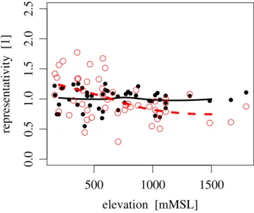
Fig. 5. Relative representativeness in geographical (black bullets)
and γ -statistical (red circles) of the observing stations of set 50. The solid black and dashed red lines are local polynomial regression fits to the bullets and circles, respectively.
be estimated and algorithmically dealt with for each interpo-lation site and network topography separately, and this is a formidable task.
Figure 5 indicates the spatial and statistical representative-ness of the observing stations of set 50. Shown are the aver-aged inverse distances to the neighboring 24 evaluating sta-tion sites (i.e. about to neighbored evaluating sites to which the observing stations are applied to in interpolation with
n=4). The geographical representativeness of the stations
scatter but is not systematically dependent on station eleva-tion. This confirms that the regularizing sub-setting has been successful. The statistical representativeness decreases with station elevation on average. Since this is not respected by geographical distance weighting and since mean observed precipitation increases with height it is expected that precip-itation will be tendencially overestimated in the Alpine area by interpolation with d-IDW. Additionally, n might be cho-sen larger or the exponents λ chocho-sen smaller in the eastern lowlands of Austria than in the Alpine area in an optimized
d-IDW interpolation setup to compensate the varying data
representativeness (not tested here).
As mentioned above the γ s also measure systematic dif-ferences in time series which may be due to elevation de-pendence of precipitation in orography, mountain shadowing effects, or horizontal trends in the precipitation field, for ex-ample. These systematic differences are not measured by the centered semi-mean squared difference
γ0α0 = 1 2T T X t =1 ((Pt0−m0) − (Pt α−mα))2 (4)
Fig. 6. Relative importance of systematic differences between pairs
of precipitation time series over geographical distance between the series sites. The black dots show the relative importance for station pairs with a vertical elevation difference of less than 50 m (only ev-ery 5th dot is drawn). The black circles show mean relative impor-tances for geographical distance classes. The same is shown by the other colored symbols but for different vertical elevation difference classes.
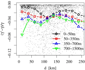
The effects of systematic differences on statistical
dis-tances are shown in Fig. 6. The relative effect (γ0−γ )/γ
over geographical distance is given for four classes of station elevation differences. For geographically nearby stations the importance of systematic differences is increasing with sta-tion elevasta-tion difference. On average the effect of systematic difference between nearby stations with almost no vertical elevation difference is below 1%. This effect is about 7 % for stations with about 1000 m vertical distance. This is con-sistent with Haiden and Stadlbacher (2002). They found for the same data an elevation dependence of yearly precipita-tion amounts up to 20% per 1000 m height difference if they restricted their evaluation to station pairs with horizontal dis-tances smaller than ten kilometers.
With increasing horizontal distance the height difference gets less important. For d≤100 km trends due to shadow-ing effects in complex terrain might be important and the remaining height correlation shown in Fig. 6 might be due to an increasing shadowing probability with larger station height differences. For even larger horizontal distances a pro-nounced east–west gradient in Austrian precipitation sums (cf. Fig. 8) might explain the increasing differences between
γ and γ0. The vertical difference dependence is probably
ar-tificial since the relative frequency of orographic heights dif-fers substantially between eastern and western Austria. Here, the possible reasons of systematic effects are not further dis-cussed, but the existence of systematic effects motivates the
usage of γ instead of γ0or R2as the statistical distance
mea-sure. In either interpolation method these trends have to be considered adequately.
The γ -IDW can be applied only at interpolation sites with long time series of precipitation observations. At non-observation sites a mixed method could be thought of. The n next neighbors are determined by geographical distance. For the neighbors long precipitation time series are available and thus their d and γ inter-distances can be determined. With this information a simple approximation for statistical dis-tances of the interpolation site to the next neighbors can be derived. Geometrical selection combined with approximated statistical distances and thus approximated statistical weights generates an interpolation method that is slightly better than
d-IDW but shall not be further discussed here. The
perfor-mance gain is small indicating that orogenic modifications on statistical distance are non-homogeneous and anisotropic in space.
4 Results
As already noted the interpolation experiments are done with the observing station data sets of size 25, 50, and 150 for the year 1999. Always 300 evaluating station sites are the considered interpolation points and thus evaluating data is available. Figure 7 compares the results of d- and γ -IDW in-terpolation. In this example the number of observing stations is 50 and next-neighbor interpolation, i.e. n=1, is applied. It is shown that often the next neighbors and thus the inter-polation values differ between the two approaches. In next-neighbor γ -IDW interpolation even two stations (Mitterfeld-alm (1665 m m.s.l.) and Filzmoos (1060 m m.s.l.) circled in Fig. 7) are not considered in interpolation. The spatial rep-resentativeness of these stations is relatively small and thus the observations at these stations are statistically useless for next-neighbor interpolation.
The interpolation results are compared to the evaluat-ing observations with simple statistics like relative bias
B=(mean(I )−mean(O))/mean(O) with I a set of
interpo-lated values and O the corresponding set of evaluating obser-vations at the interpolation sites, linear correlation R(I, O), the ratio of standard deviations σ (I )/σ (O), and efficiency
E=1−mean((I −O)2)/σ2(O)=1−MSE(I, O)/σ2(O).
The spatial average of time series biases is denoted by Bt.
and the temporal average of biases between daily
precip-itation fields is denoted B.s. The dot indicates the finally
averaged dimension. The same notation is applied to the av-eraged correlations, standard deviations and efficiencies. In case of perfect interpolation the values of the bias statistics are identical zero and the other statistics’ values are one.
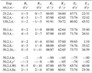
Table 2 shows mean results of the evaluation. As expected the correlation of interpolated values with evaluating data in-creases with the number of observing stations. Improvement of bias is not that obvious. Changes in the exponent λ have a smaller impact, but are not unimportant. The evaluation
Fig. 7. IDW interpolation of data measured at 50 observing stations for 19 August 1999. The color of the bullets at the station sites (marked
with +) show the observed values. These are a subset of the observations shown in Fig. 2. The squares indicate the interpolation points with the outline color giving the interpolation results by standard next–neighbor geographical IDW and the filling color giving next–neighbor
γ-IDW results. The arrows point to the interpolation stations highlighted in Fig. 4. The circles mark observing stations not considered in
next-neighbor γ -interpolation.
indicates that in d-IDW an exponent smaller than two per-forms best in the yearly average. More important is the num-ber n of considered observation neighbors. In case of 50 observing stations four-neighbor interpolation is better than next-neighbor interpolation but there is no relevant improve-ment in taking eight neighbors and even slight decrease in interpolation performance if sixteen neighbors are taken. A similar number of neighbors are optimal in case of 25 or 150 observing stations.
The γ -IDW interpolation is better in correlation and effi-ciency but seems to be worse in bias. In d-interpolation there is a more pronounced spatial compensation of errors. Under-estimation, for example close to the southern Austrian border (cf. Fig. 8), is compensated by a tendency for overestimation in central Alpine areas by geographical interpolation. This is due to overestimation of representativeness of high-elevation observations (cf. Fig. 5). The tendency for underestimation in γ -interpolation can be avoided if the statistical distances are estimated after logarithmic transformation of the time se-ries (cf. experiment ln in Table 2). This effectively reduces the positive skewness of the intensity distribution of daily precipitation. The skewness of the precipitation distribution is an important problem common to all interpolation meth-ods, but shall not be discussed further in the present context. Figure 8 shows the relative biases of the interpolating time series with next-neighbor d- or γ -distance interpolation. The
Table 2. Mean evaluation results of interpolation experiments. The
table gives the spatial mean of relative time series biases Bt., the
temporal mean of spatial biases is B.s, and the related correlation
coefficients Rt. and R.s and efficiencies. All values are given in
percent and thus the values of Bs would be 0 and all other values would be 100 in case of perfect interpolation.
Exp. Bt. B.s Rt. R.s Et. E.s set,λ,n,– d/γ d/γ d/ γ d/ γ d/γ d/γ 25,2,4,– 1/−5 0/−7 84/85 56/60 67/71 22/33 50,2,4,– 4/−3 1/−7 87/88 62/65 73/76 32/42 150,2,4,– 1/−2 −1/−5 91/91 70/72 80/82 45/52 50,1,4,– 4/−2 1/−8 88/88 62/64 73/76 35/40 50,3,4,– 4/−3 2/−7 87/88 61/65 71/76 26/41 50,2,1,– 4/−2 4/−6 83/84 57/60 59/65 1/19 50,2,8,– 4/−3 1/−8 88/88 63/65 74/76 35/42 50,2,16,– 5/−5 1/−11 88/87 62/65 73/73 36/39 50,2,4,ln −/2 −/0 −/88 −/65 −/75 −/40 50,2,4,γ0 −/−3 −/−8 −/88 −/65 −/76 −/42 50,2,4,Wi 9/−5 0/−10 87/88 65/70 65/74 40/48 50,2,4,Su 2/−1 2/−6 87/88 60/61 73/76 25/36
Fig. 8. As Fig. 7 but showing precipitation sums for the year 1999 at 50 observation sites and relative biases at the evaluation sites. The
vertical bars indicate relative biases for the 1999 interpolation experiments. The inlet shows the height of a bar with 100% positive bias. Black gives biases with geographical and red with statistical distance next-neighbor interpolation.
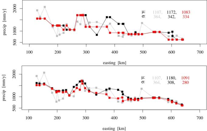
spatial averages of these biases are given in Table 2 by exper-iment 50/2/1/– to 4 and −2, respectively. Obviously, relative biases in d-IDW interpolation are larger in mountainous ter-rain than in the lowlands (the same is valid for correlation and efficiency errors, not shown). In mountainous terrain the scatter in relative biases is smaller with γ - instead of d-interpolation and thus performance of γ -d-interpolation is bet-ter. This can also be seen in Fig. 9. This figure shows interpo-lated precipitation sums in comparison with observed sums of 1999 in a west-east transection with areal support of 350 to 370 km northing. Results with next- and four-neighbors in-terpolation are compared. Again the tendencies of over– and underestimation of geographical or statistical distance inter-polation are visible. The tendency of smaller values of sta-tistical interpolation yields smaller standard deviations. Sub-jectively interpolation with n=4 leads to better results, but obviously also to smoother, variability vastly underestimat-ing fields.
The smaller scatter in bias, correlation and efficiency by
γ-IDW is also shown by the histograms in Fig. 10. These
histograms give statistics values applying n=4 interpolation. The statistical distance interpolation is more robust than ge-ographical distance interpolation. Extreme overestimates of daily means are avoided. Correlations are shifted to higher
values and the number of days with spatial R2≤0.5 and small
or even useless (E≤0) efficiencies are significantly reduced. Obviously, time series performance is better than spatial
performance. This is due to the scales of the data. The tem-poral support of the data is daily. The spatial support of the
observations (∼1000 cm2) is very small in comparison
(Or-lanski, 1975). This explains the better performance of inter-polation in terms of time series than of spatial field compar-isons. As a consequence the spatial results are more sensitive to the chosen interpolation method.
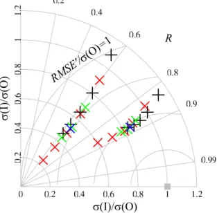
Most interpolation methods are smoothing operations which reduce field variability. This is visualized in the Tay-lor (2001)-diagram shown in Fig. 11. For example, next-neighbor d-interpolation overestimates temporal and spatial variability in comparison with the evaluating observations. But, with n=2, 4 etc. variability is more and more underes-timated. This effect is more important for spatial than tem-poral variability because of the relatively smaller spatial in-terpolation support scale. The traces of crosses in the di-agram are convex showing that there is an optimum number of neighbors to be considered in interpolation. If in the envis-aged application the field correlation is more important than field variability then a number of four neighbors is well cho-sen in case of 50 observing stations. The optimum depends on the interpolation setup: number of stations, power of dis-tance, spatial and temporal variability of the natural precip-itation field etc. The impact on smoothing of the power λ of the distance and de-skewing in γ -IDW are also shown in Fig. 11. With increasing λ the effective number of obser-vations decrease and variability of the interpolating values
100 200 300 400 500 600 700 500 1000 2000 easting [km] precip [mm/y] µ : σ : 1107,364, 1172,342, 1083334 100 200 300 400 500 600 700 500 1000 2000 easting [km] precip [mm/y] µ : σ : 1107,364, 1180,308, 1091280
Fig. 9. Year 1999 sums of observed and interpolated precipitation at sites in a west-east transection with areal support between 350 and
370 km northing. Grey symbols show the observed values, black symbols the interpolated values with geographical distance interpolation and red symbols with statistical distance interpolation respectively. The upper panel applies n=1, i.e. next-neighbor, and the lower panel applies n=4 neighbors in interpolation. The transection means µ and standard deviations σ are given too.
increase. De-skewing in γ estimation slightly improves vari-ability, correlation and thus (as is proven in Taylor, 2001)
centered root-mean-square error RMSE0.
As discussed earlier there are systematic differences be-tween station time series due to vertical or horizontal trends. In the interpolation experiments on a daily data basis these systematic effects are generally small in comparison to
in-terpolation errors as is shown by application of γ0instead of
γ distances (cf. experiment γ0 in Table 2). This says that
on average the relative importance of vertical dependence of precipitation rates is small in comparison with interpolation errors in our setup. Of course, in some areas or applications the vertical dependence is important. Additionally, these sys-tematic effects get more important with increasing interpola-tion performance, for example because of increasing tempo-ral support of interpolation time slices (i.e. monthly or yearly precipitation fields instead of daily fields).
Seasonal stratification of precipitation events in γ -estimation and -interpolation yields the expected results. Ta-ble 2 gives interpolation results if only Summer or Win-ter six-month data are considered (experiments Su and Wi). Spatial field correlations and efficiencies are better in Winter than in Summer. In Austria the Winter precipitation is less intensive and less heterogeneous in the mean than Summer
precipitation. The more stochastic character of convective Summer rain reduces the spatial representativeness of data. Nonetheless, the temporal correlation differences are small.
Interestingly, the temporal efficiencies are even better in
Summer than in Winter. The MSEs of the interpolated
time series are smaller in Winter (d: 7.6 (mm/d)2 and γ :
5.9 (mm/d)2) than in Summer (d: 17.9 (mm/d)2 and γ :
15.9 (mm/d)2). But, if the MSEs are normalized with
ob-served time series mean variance (22 and 66 (mm/d)2 in
Winter and Summer, respectively) then Summer interpola-tion performs better than Winter interpolainterpola-tion in terms of time series comparison. In either case, Summer or Winter,
γ-IDW performs better than d-IDW with performance gain
more pronounced in Winter because of higher stationarity of spatial patterns caused by frontal interaction with orography. Stratification of precipitation days with a mean wind di-rection classification for the lower atmospheric levels in the Eastern Alps (Steinacker, 1990) has been tried also. This even slightly reduces overall performance in γ interpola-tion. The small scale γ -distances are not highly dependent on large scale wind direction. Additionally, the size of specific wind direction classes is small even in the available thirty year data sets and thus estimation of stratified γ s is not ro-bust.
206 B. Ahrens: Distance in spatial interpolation of daily rain gauge data Bt. [%] frequency −100 0 100 200 300 0 50 100 150 Rt. frequency 0.0 0.2 0.4 0.6 0.8 1.0 0 50 100 150 Et. frequency −1.0 −0.5 0.0 0.5 1.0 0 50 100 150 B.s [%] frequency −100 0 100 200 300 0 50 100 150 R.s frequency 0.0 0.2 0.4 0.6 0.8 1.0 0 50 100 150 E.s frequency −1.0 −0.5 0.0 0.5 1.0 0 50 100 150 Bt. [%] frequency −100 0 100 200 300 0 50 100 Rt. frequency 0.0 0.2 0.4 0.6 0.8 1.0 0 50 100 Et. frequency −1.0 −0.5 0.0 0.5 1.0 0 50 100 B.s [%] frequency −100 0 100 200 300 0 50 100 150 R.s frequency 0.0 0.2 0.4 0.6 0.8 1.0 0 50 100 150 E.s frequency −1.0 −0.5 0.0 0.5 1.0 0 50 100 150
Fig. 10. Histograms of spatially (upper row) and temporally (lower row) averaged statistics. The solid red histograms show the evaluation
results for γ - and the hatched black histograms for the d-distance interpolation with set 50, n=4, and γ =2.
R
σ
(I)/σ(O)
σ
(I)/
σ
(O)
RM
SE
'/σ
(O)
=1
Fig. 11. Taylor (2001)-diagram showing evaluation results with
ob-servation set 50 but different interpolation setups. Black “+” and red “x” show the dependency on n with n=1, 2, 4, 8, 16 for d- and
γ-interpolation, respectively, and γ =2. The green “x” show results
with γ -interpolation and n=4 and γ =1, 3, 4. The blue “x” show results for experiment ln. The group of symbols indicating better
correlations and centered RMSE0s are from time series comparisons
and the other group indicate spatial field comparisons.
5 Conclusions
Spatial interpolation of daily rain gauge data with Inverse Distance Weighting (IDW) at locations with available precip-itation time series has been investigated. It has been shown that the application of a statistical distance measure between neighbored precipitation time series instead of geographical distances between station locations slightly improves aver-aged interpolation performance. The main advantage is that statistical distance IDW is more robust especially in or close to mountainous terrain where complex rain–orography inter-action is important that is implicitly considered in the sta-tistical distance. This performance gain in mountainous ter-rain illustrates the potential of simple but necessarily spa-tially highly resolving models of rain-orography interaction. Geostatistical interpolation methods consider statistical re-lationship between stations through variogram or correlation models. Often, geostatistical models are implemented lo-cally, i.e. they consider n next neighbors in interpolation. These n neighbors could easily be selected by explicit use of statistical distance. More sophisticated approaches could be thought of. For example, Kriging could be applied after mapping station locations with statistical distances instead of geographical distances by metric multidimensional scaling (Sammon, 1969). Thus, standard Kriging could be applied in statistical space, but this is a topic for further research.
Implementation of IDW interpolation with statistical dis-tance is easily done if the necessary time series are available at the interpolation sites. An example of application might be
150 rain gauges with daily or better resolution are available to the Austrian national weather service. Following Weil-guni (2003) about 950 additional rain gauges with daily mea-surements are operated in Austria by the hydrological ser-vice, hydropower agencies etc. These additional stations are not available in near real-time, but their statistical informa-tion could be applied easily within the statistical IDW. This would be a parsimonious and robust procedure for using all available rain gauge data in densification of the point data network that could be appropriately upscaled in precipitation mapping.
Acknowledgements. Data are provided by the Hydrographische
Zentralb¨uro, BMLFUW, Vienna. The author is funded by the
Austrian Academy of Sciences.
Edited by: L. G. Lanza
References
Adler, R. F., Kidd, C., Petty, G., Morissey, M., and Goodman, H. M.: Intercomparison of Global Precipitation Products: The Third Precipitation Intercomparison Project (PIP-3), Bull. Amer. Meteorol. Soc., 82, 1377–1396, 2001.
Auer, I., B¨ohm, R., Jurkovi´c, A., Orlik, A., Potzmann, R., Sch¨oner, W., Ungersb¨ock, M., Brunetti, M., Nanni, T., Magueri, M., Briffa, K., Jones, P., Efthymiadis, D., Mestre, O., Moisselin, J.-M., Begert, J.-M., Brazdil, R., Bochnic´ek, O., Cegnar, T., Gaji´c-Capka, M., Zaninovi´c, K., Majstorovi´c, C., Szalai, S., Szentim-rey, T., and Mercalli, L.: A new instrumental precipitation dataset for the greater Alpine region for the period 1800–2002, Int. J. Climatol., 25, 139–166, doi:10.1002/joc.1135, 2005.
Barros, A. P. and Lettenmaier, D. P.: Dynamic Modeling of oro-graphically induced precipitation, Rev. Geophys., 32, 265–284, 1994.
Beck, A., Ahrens, B., and Stadlbacher, K.: Impact of
nest-ing strategies on precipitation forecastnest-ing in dynamical down-scaling of reanalysis data, Geophys. Res. Lett., 31, 5, doi:10.1029/2004GL020115, 2004.
Bl¨oschl, G. and Grayson, R.: Spatial Observations and interpola-tion, in: Spatial patterns in catchment hydrology: observations and modelling, edited by: Grayson, R. and Bl¨oschl, G., Cam-bridge University Press, UK, ISBN 0-521-63316-8, 17–50, 2001. Ciach, G., Morrissey, M., and Krajewski, W. F.: Conditional bias in radar rainfall estimation, J. Appl. Meteorol., 39, 1941–1946, 2000.
Creutin, J. D. and Obled, C.: Objective analyses and mapping tech-niques for rainfall fields: An objective comparison, Water Re-sour. Res., 18, 413–431, 1982.
Daly, C., Neilson, R., and Phillips, D.: A statistical-topographic model for mapping climatological precipitation over mountain-ous terrain, J. Appl. Meteorol., 33, 140–158, 1994.
Durand, Y., Brun, E., M´erindol, L., Guyomarc’h, G., Lesafre, B., and Martin, E.: A meteorological estimation of relevant param-eters for snow schemes used with atmospheric models, Ann. Glaciol., 18, 65–71, 1993.
N. J.: Creating a serially complete, national daily time series of temperature and precipitation for the Western United States, J. Appl. Meteorol., 39, 1580–1591, 2000.
Frei, C. and Sch¨ar, C.: A precipitation climatology of the Alps from high-resolution rain-gauge observations, Int. J. Climatol., 18, 873–900, 1998.
Haiden, T. and Stadlbacher, K.: Quantitative Prognose des
F¨achenniederschlags, ¨Osterr. Wasser- und Abfallwirtschaft, 10,
135–141, 2002.
Liebmann, B. and Allured, D.: Daily precipitation grids for
South America, Bull. Amer. Meteorol. Soc., 86, 1567–1570, doi:10.1175/BAMS-86-11-1567, 2005.
Orlanski, I.: A rational subdivision of scales for atmospheric pro-cesses, Bull. Amer. Meteorol. Soc., 56, 527–530, 1975. Palecki, M. A., Angel, J. R., and Hollinger, S. E.: Storm
precipita-tion in the United States. Part I: Meteorological characteristics, J. Appl. Meteorol., 44, 933–946, doi:10.1175/JAM2243.1, 2005.
Rubel, F.: PIDCAP Quick look precipitation atlas, vol. 15 of ¨Osterr.
Beitr. Meteorol. Geophys., ZAMG, Wien, 1996.
Rubel, F. and Hantel, M.: BALTEX 1/6-degree daily precipitation climatology 1996–1998, Meteorol. Atmos. Phys., 77, 155–166, 2001.
Rudolf, B. and Rubel, F.: Global precipitation, in: Observed Global Climate, edited by: M. Hantel, Landolt-B¨ornstein: Numerical Data and Functional Relationships in Science and Technology – New Series, Group 5: Geophysics, 6(A), 11.1–11.53, Springer, Berlin, 2005.
Sammon Jr., J.: A nonlinear mapping for data structure analysis, IEEE Trans. Comput., C-18, 401–409, 1969.
Scheifinger, H., B¨ohm, R., and Auer, I.: R¨aumliche Dekorrela-tion von Klimazeitreihen unterschiedlicher zeitlicher Aufl¨osung und ihre Bedeutung f¨ur ihre Homogenisierbarkeit und die Repr¨asentativit¨at von Ergebnissen, in Proceedings of 6. Deutsche Klimatagung, Klimavariabilit¨at 2003, 22–25 September 2003, Potsdam, no. 6 in Terra Nostra, Schriftenreihe der Alfred-Wegener-Stiftung, pp. 375–379, 2003.
Sevruk, B.: Regional dependency of precipitation–altitude relation-ship in the Swiss Alps, Climatic Change, 36, 355–369, 1997. Shepard, D.: Computer mapping: The SYMAP interpolation
al-gorithm, in: Spatial statistics and models, edited by: Gaile, G. and Willmott, C., Dordrecht, Reidel Publishing, p. 95–116, 1984.
Singh, V. and Frevert, D. (Eds.): Mathematical Models of
Large Watershed Hydrology, Water resources Publications, LLC, Chelsea, Michigan, 2002a.
Singh, V. and Frevert, D. (Eds.): Mathematical Models of Small Watershed Hydrology and Applications, Water resources Publi-cations, LLC, Chelsea, Michigan, 2002b.
Skoda, G., Weilguni, V., and Haiden, T.: Heavy convective storms – Precipitation during 15, 60, and 180 minutes, chap. 2.5–7, Hy-drological Atlas of Austria, Bundesministerium f¨ur Land- und Forstwirtschaft, Umwelt und Wasserwirtschaft, 2003.
Smith, R.: The influence of mountains on the atmosphere, Adv. Geophys., 21, 87–230, 1979.
Smith, R.: A linear upslope-time-delay model for orographic pre-cipitation, J. Hydrol., 282, 2–9, 2003.
Steinacker, R.: Eine ostalpine Str¨omungslagenklassifikation, Tech. rep., IMG; Universit¨at Wien, Austria, http://www.univie.ac.at/ IMG-Wien/weatherregime/, pp. 8, 1990.
Taylor, K.: Summarizing multiple aspects of model performance in a single diagram, J. Geophys. Res., 106, 7183–7192, 2001. Tobler, W.: A computer movie simulating urban growth in the
De-troit region, Economic Geography, 46, 234–240, 1970.
Weilguni, V.: Precipitation stations, chap. 2.1, Hydrological At-las of Austria, Bundesministerium f¨ur Land- und Forstwirtschaft, Umwelt und Wasserwirtschaft, 2003.
Young, C., Nelson, B., Bradley, A., Smith, J., Peters-Lidard, C., Kruger, A., and Baeck, M.: An evaluation of NEXRAD pre-cipitation estimates in complex terrain, J. Geophys. Res., 104, 19 691–19 703, 1999.