ENSO surface longwave radiation forcing over the tropical Pacific

HAL Id: hal-00296199

https://hal.archives-ouvertes.fr/hal-00296199

Submitted on 24 Apr 2007

HAL is a multi-disciplinary open access

archive for the deposit and dissemination of

sci-entific research documents, whether they are

pub-lished or not. The documents may come from

teaching and research institutions in France or

abroad, or from public or private research centers.

L’archive ouverte pluridisciplinaire HAL, est

destinée au dépôt et à la diffusion de documents

scientifiques de niveau recherche, publiés ou non,

émanant des établissements d’enseignement et de

recherche français ou étrangers, des laboratoires

publics ou privés.

tropical Pacific

K. G. Pavlakis, D. Hatzidimitriou, E. Drakakis, C. Matsoukas, A. Fotiadi, N.

Hatzianastassiou, I. Vardavas

To cite this version:

K. G. Pavlakis, D. Hatzidimitriou, E. Drakakis, C. Matsoukas, A. Fotiadi, et al.. ENSO surface

longwave radiation forcing over the tropical Pacific. Atmospheric Chemistry and Physics, European

Geosciences Union, 2007, 7 (8), pp.2013-2026. �hal-00296199�

www.atmos-chem-phys.net/7/2013/2007/ © Author(s) 2007. This work is licensed under a Creative Commons License.

Chemistry

and Physics

ENSO surface longwave radiation forcing over the tropical Pacific

K. G. Pavlakis1,2,3, D. Hatzidimitriou1,3, E. Drakakis1,4, C. Matsoukas1,6, A. Fotiadi3, N. Hatzianastassiou1,5, and I. Vardavas1,3

1_{Foundation for Research and Technology-Hellas, Heraklion, Crete, Greece}

2_{Department of General Applied Science, Technological Educational Institute of Crete, Greece} 3_{Department of Physics, University of Crete, Crete, Greece}

4_{Department of Electrical Engineering, Technological Educational Institute of Crete, Greece} 5_{Laboratory of Meteorology, Department of Physics, University of Ioannina, Greece} 6_{Department of Environment, University of the Aegean, Greece}

Received: 25 July 2006 – Published in Atmos. Chem. Phys. Discuss.: 11 December 2006 Revised: 22 February 2007 – Accepted: 2 April 2007 – Published: 24 April 2007

Abstract. We have studied the spatial and temporal

varia-tion of the surface longwave radiavaria-tion (downwelling and net) over a 21-year period in the tropical and subtropical Pacific Ocean (40 S–40 N, 90 E-75 W). The fluxes were computed using a deterministic model for atmospheric radiation trans-fer, along with satellite data from the ISCCP-D2 database and reanalysis data from NCEP/NCAR (acronyms explained in main text), for the key atmospheric and surface input pa-rameters. An excellent correlation was found between the downwelling longwave radiation (DLR) anomaly and the Ni˜no-3.4 index time-series, over the Ni˜no-3.4 region located in the central Pacific. A high anti-correlation was also found over the western Pacific (15–0 S, 105–130 E). There is con-vincing evidence that the time series of the mean down-welling longwave radiation anomaly in the western Pacific precedes that in the Ni˜no-3.4 region by 3–4 months. Thus, the downwelling longwave radiation anomaly is a comple-mentary index to the SST anomaly for the study of ENSO events and can be used to asses whether or not El Ni˜no or La Ni˜na conditions prevail. Over the Ni˜no-3.4 region, the mean DLR anomaly values range from +20 Wm−2 dur-ing El Ni˜no episodes to −20 Wm−2during La Ni˜na events, while over the western Pacific (15–0 S, 105–130 E) these val-ues range from −15 Wm−2to +10 Wm−2, respectively. The long- term average (1984–2004) distribution of the net down-welling longwave radiation at the surface over the tropical and subtropical Pacific for the three month period November-December-January shows a net thermal cooling of the ocean surface. When El Ni˜no conditions prevail, the thermal radia-tive cooling in the central and south-eastern tropical Pacific becomes weaker by 10 Wm−2south of the equator in the

cen-Correspondence to: K. Pavlakis

(pavlakis@iesl.forth.gr)

tral Pacific (7–0 S, 160–120 W) for the three-month period of NDJ, because the DLR increase is larger than the increase in surface thermal emission. In contrast, the thermal radiative cooling over Indonesia is enhanced by 10 Wm−2during the early (August–September–October) El Ni˜no phase.

1 Introduction

The El Ni˜no Southern Oscillation (ENSO) is a natural cy-cle that couples the ocean-atmosphere system over the trop-ical Pacific and operates on a timescale of 2–7 years. Once developed, it causes a shift in the seasonal temperature and precipitation patterns in many different regions of the world, since heating of the tropical atmosphere creates changes in the global atmospheric circulation. Thus, ENSO is a dom-inant source of inter-annual climate variability around the world. Following the early work of Bjerknes (1966, 1969) who attributed ENSO to coupled Pacific ocean-atmosphere interactions, the dynamics of this pattern of climate variabil-ity was extensively studied by many workers (e.g. Philander, 1990; McCreary and Anderson, 1991; Neelin et al., 1998). Normally, the equatorial Pacific Ocean is characterized by warm waters in the west and cold waters in the east. The ENSO warm phase (El Ni˜no) is associated with an unusual warming of the eastern and central equatorial Pacific accom-panied by a shift in the deep atmospheric convection from the western Pacific to the equatorial central Pacific. La Ni˜na, the ENSO cold phase, is the counterpart to El Ni˜no, often following it. It is characterised by cooler than normal sea surface temperatures across the equatorial eastern Pacific and a strengthening of near ocean-surface winds travelling from east to west. Thus ENSO is an oscillation between warm

and cold events with a peak that typically occurs late in the calendar year (late December-early January). Both El Ni˜no and La Ni˜na events last for about a year, but they can last for as long as 18 months (see the recent review by Wang and Fiedler, 2006). Over the past two decades a large number of studies have appeared, attempting to explain the mechanism of the oscillation between the two phases of the ENSO phe-nomenon and many models have been proposed (e.g. Suarez and Schopf, 1988; Cane et al., 1990; Jin, 1997a, b; Picaut et al., 1997; Wang et al., 1999; Wang, 2001). A recent short review summarizing theories and mechanisms about El Ni˜no variability is given by Dijkstra (2006).

During ENSO, a feedback between atmospheric and ocean properties is observed. Sea surface temperature (SST) anomalies induce wind stress anomaly patterns that in turn produce a positive feedback on the SST. Variation of the above properties cause significant changes in other oceanic and atmospheric variables, e.g. the mean depth of the ther-mocline, the water vapour content of the atmosphere and the relative distributions of low, middle and high clouds. Wa-ter vapour and clouds are the main regulators of the radia-tive heating of the planet since changes in these parameters modulate the variability in the radiation fluxes that regulate the heating or cooling of the Earth’s surface and atmosphere (Tian and Ramanathan, 2002). The radiation field in turn, fluences SST and atmospheric water vapour. Thus ENSO in-volves complex climatic processes and feedbacks that make its onset time, duration, strength and spatial structure dif-ficult to predict (see Fedorov et al., 2003, and references therein). International monitoring programmes of the cou-pled atmosphere-ocean system started in the Pacific around 1985 and led to the TAO/TRITON (Tropical Atmosphere Ocean project/Triangle Trans Ocean Buoy Network) array of moored buoys. The aim of this programme is to provide real-time measurements of winds, sea surface temperature, subsurface temperature, sea level and ocean flow that help in the understanding of the physical processes responsible for ENSO (McPhaden et al., 1998).

The variability and the spatial distribution of the ocean and atmospheric variables are not the same for all ENSO events. Thus a definition of ENSO is necessary for the study of this phenomenon (Trenberth, 1997). The phase and strength of ENSO events are defined by an index. Several different in-dices have been used in the literature, mostly based on SST, although there is one index, the Southern Oscillation index, which is related to air pressure differences at sea level, be-tween Darwin (Australia) in the west and Tahiti in the east. The SST based indices are obtained from the SST anomalies with respect to average values over some specified region of the ocean (see for example, Trenberth and Stepaniak, 2000; Hanley et al., 2003). There has been also an effort to combine several atmospheric-oceanic variables into a single index like the multivariate ENSO index (Wolter and Timlin, 1998). Av-erages of 850 mb wind, outgoing longwave radiation (OLR) at the top of the atmosphere as well as precipitation over

spe-cific regions (Curtis and Adler, 2000) are also used, although not often, to monitor ENSO.

The Earth’s climate system is driven by the radiative en-ergy balance between the solar shortwave radiation (SW) ab-sorbed by the atmosphere and the surface of the Earth and the thermal longwave radiation (LW) emitted by the Earth to space. In this respect, ENSO events are expected to be asso-ciated with the spatial and temporal variability of the radia-tive energy balance over the tropical and subtropical Pacific. The net heat flux into the ocean plays a key role in ENSO evolution and is a significant variable in the models that have been developed to make ENSO predictions (Dijkstra, 2006). The variation of the net heat flux during ENSO events is of paramount importance to the dynamics of the system (Har-rison et al., 2002; Chou et al., 2004). The net heat flux into the ocean is a small residual of four terms, the downward shortwave radiation at the surface (DSR), the latent heat loss, the sensible heat transfer and the net downwelling longwave radiation at the Earth’s surface (NSL). The NSL is the dif-ference between the downward longwave radiation (DLR) at the Earth’s surface and the Earth’s surface thermal emission. The DLR at the Earth’s surface is a very important compo-nent of the surface radiation budget with variations arising from increases in greenhouse gases or from changes in other atmospheric properties that occur during ENSO events (In-tergovernmental Panel on Climate Change, IPCC, 2001). In this work we shall focus on the behaviour of the DLR and NSL during warm and cold ENSO events over the tropical and subtropical Pacific Ocean. The DLR depends mainly on the vertical distributions of temperature and water vapour in the lower troposphere, as well as on the cloud amounts and cloud radiative properties. We shall show that the DLR is a very useful index for the description of the phase and evolu-tion of ENSO events.

We present DLR and NSL data generated by a determinis-tic radiation transfer model for the period 1984–2004 for the tropical and subtropical Pacific Ocean and examine their spa-tial and temporal variability during ENSO events. In addi-tion, we investigate the correlation of DLR and NSL anoma-lies with the Ni˜no 3.4 index. In Sect. 2 we describe the radi-ation model and the input data used. In Sect. 3, the surface longwave radiation distribution and its variation during warm and cold ENSO phases are presented. In Sect. 4, the DLR and NSL variation during ENSO evolution is examined. In Sect. 5, the correlation of the Ni˜no 3.4 index and surface ra-diation parameters are presented while in Sect. 6 a more de-tailed analysis of radiation parameters in the western Pacific is presented. In Sect. 7, we discuss our results and in Sect. 8 we present our conclusions. Table 1 lists the symbol defini-tions of the radiation parameters that are most often used in this paper.

2 Radiation model and data description

We use the FORTH deterministic model (Pavlakis et al., 2004) for the radiation transfer of terrestrial infrared ra-diation, to compute the downward longwave radiation at the surface of the Earth (DLR). This model is based on a detailed radiative-convective model developed for climate change studies (Vardavas and Carver 1984), but modified in order to model the longwave atmospheric radiation fluxes at the Earth’s surface and at top of atmosphere (TOA), on a 2.5◦×2.5◦grid for the entire globe.

The model DLR has a temporal resolution of one month, and a vertical resolution (from the surface up to 50 mb) of 5 mb, to ensure that the atmospheric layers are optically thin with respect to the Planck mean longwave opacity. The at-mospheric molecules considered are; H2O, CO2, CH4, O3, and N2O. The sky is divided into clear and cloudy frac-tions. The cloudy fraction includes three non-overlapping layers of low, mid and high-level clouds. Expressions for the fluxes for clear and cloudy sky can be found in Hatzianas-tassiou et al. (1999). The model input data include cloud amounts (for low, mid, high-level clouds), cloud absorption optical depth, cloud-top pressure and temperature (for each cloud type), cloud geometrical thickness and vertical temper-ature and specific humidity profiles. For the total amount of ozone, carbon dioxide, methane, and nitrous oxide in the at-mosphere, we used the same values as in Hatzianastassiou and Vardavas (2001).

All of the cloud climatological data for our radiation transfer model were taken from the International Satellite Cloud Climatology Project (ISCCP-D2) data set (Rossow and Schiffer, 1999), which provides monthly means for 72 climatological variables in 2.5-degree equal-angle grid-boxes for the period 1984–2004. The vertical distributions of the temperature and water vapour as well as the sur-face temperature, were taken from the National Center for Environmental Prediction/National Centers for Atmospheric Research (NCEP/NCAR) reanalysis project (Kistler et al., 2001), corrected for topography as in Hatzianastassiou et al. (2001). These data are also on a 2.5-degree resolution, monthly averaged and cover the same 21-year period as the ISCCP-D2 data.

A full presentation and discussion of the model and DLR distribution can be found in Pavlakis et al. (2004). There, a series of sensitivity tests were performed to investigate how much uncertainty is introduced in the model DLR by uncer-tainties in the input parameters, such as air temperature, skin temperature, low, middle or high cloud amount as well as the cloud physical thickness, cloud overlap schemes, and the use of daily-mean instead of monthly-mean input data. The model DLR was also validated against BSRN station mea-surements for the entire globe (Pavlakis et al., 2004; Mat-soukas et al., 2005).

(a)

(b)

(c)

Fig. 1. The distribution of downward longwave radiation (DLR),

over tropical and subtropical Pacific for the three month pe-riod November, December, January (NDJ); (a) long-term average (1984–2004), (b) average for five El Ni˜no years, (c) average for five La Ni˜na years.

3 Long-term surface longwave radiation

The geographical distribution of the 21-year average (1984– 2004) DLR at the surface, over the tropical and subtrop-ical Pacific Ocean (40 S–40 N, 90 E–75 W), with a spatial

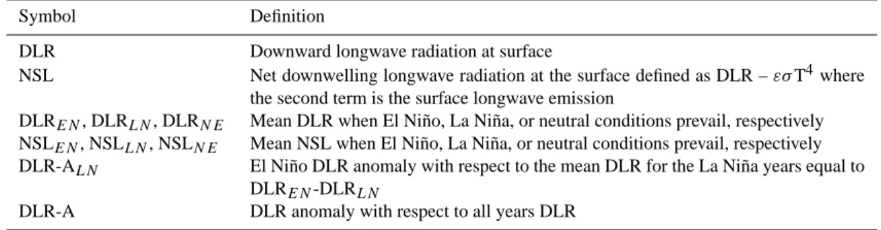
Table 1. Definition of symbols used to represent radiation parameters.

Symbol Definition

DLR Downward longwave radiation at surface

NSL Net downwelling longwave radiation at the surface defined as DLR – εσ T4where the second term is the surface longwave emission

DLREN, DLRLN, DLRN E Mean DLR when El Ni˜no, La Ni˜na, or neutral conditions prevail, respectively

NSLEN, NSLLN, NSLN E Mean NSL when El Ni˜no, La Ni˜na, or neutral conditions prevail, respectively

DLR-A_LN El Ni˜no DLR anomaly with respect to the mean DLR for the La Ni˜na years equal to DLREN-DLRLN

DLR-A DLR anomaly with respect to all years DLR

resolution of 2.5◦(latitude)×2.5◦(longitude), is shown in Fig. 1 top panel (a), for the 3-month period November, De-cember and January (NDJ). The three month period NDJ is selected as best representing the mature phase of ENSO evo-lution, as the ENSO peak typically occurs late in the calen-dar year (December–January). It is within this period that the strongest changes in the DLR occur (see Sect. 4).

The five significant El Ni˜no events in our 21-year study period, 1984–2004, were during 1986–1987, 1991–1992, 1994–1995, 1997–1998 and 2002–2003. In the same period, the more significant La Ni˜na events were during 1984–1985, 1988–1989, 1998–1999, 1999–2000, 2000–2001 (Trenberth, 1997; Wang and Fiedler, 2006). We have calculated, for each grid-box, the mean monthly DLR averaged over the 11 neu-tral years (DLRN E), i.e. the years when no significant El Ni˜no or La Ni˜na events occurred for the period NDJ. Both the long-term mean DLR and the DLRN E for NDJ show similar spatial patterns and their values have differences less than 5 Wm−2. Thus only the long-term mean DLR is shown, which is representative of normal conditions. As expected, the maxima in DLR, reaching about 430 Wm−2, occur over the western Pacific, where the Western Pacific Warm Pool is located. The highest open ocean water temperatures on Earth are observed there. Because of these high temperatures, the atmosphere is supplied with large amounts of water vapour, the most important greenhouse gas, resulting in high DLR values.

We also computed, for each grid-box, the average DLR over the five years1when El Ni˜no (DLREN)conditions pre-vailed (Fig. 1, middle panel b) and the corresponding average DLR over the five years when La Ni˜na (DLRLN)conditions prevailed (Fig. 1, bottom panel c), for the three month pe-riod of NDJ. It is evident from these figures that high values of DLR are observed over much more extended areas of the central and eastern Pacific, during the El Ni˜no years com-pared to the La Ni˜na average.

In Fig. 2, top panel (a) we show the geographical distri-bution of the 21-year average (1984–2004) net downwelling 1_{An “El Ni˜no year” is defined, for our purposes, as starting in}

July and ending in June of the next year.

longwave radiation at the surface (NSL) for the three-month period NDJ. The NSL is defined as NSL=DLR–εσ T4, where

εσT4 is the surface longwave emission, ε is the ocean face emissivity taken to be 0.95 and T is the SST. The sur-face emissivity for non-oceanic areas was computed by us-ing surface-type cover fractions from the ISCCP-D2 database and the land surface emissivity set to 0.9. We have also cal-culated, for each grid-box, the mean monthly NSL for NDJ averaged over the 11 neutral years (NSLN E). The NSL and NSLN E show similar values over the tropical and subtropi-cal Pacific thus only the long-term NSL is presented in Fig. 2, which is representative of normal conditions. Clearly, NSL is negative over most of the region. The highest negative val-ues, reaching 40–45 Wm−2, occur in the central and south-eastern Pacific.

In Fig. 2 are also shown the average NSL over the five years when El Ni˜no (NSLEN)conditions prevailed for NDJ (middle panel b), and the corresponding average NSL over the five years when La Ni˜na (NSLLN)conditions prevailed (bottom panel c). It is clear from these figures that when El Ni˜no conditions prevail, the thermal radiative cooling in the central and south-eastern tropical Pacific becomes weaker.

During ENSO warm (El Ni˜no) or cold (La Ni˜na) phases, the equatorial Pacific warms or cools, respectively, by as much as 3◦C. This warming or cooling of the Pacific ocean is accompanied by significant changes in DLR and NSL, as shown in Figs. 1 and 2, indicating a significant change in the longwave radiation budget of the region.

In Fig. 3a we show the distribution of the difference DLREN–DLRLN, over the tropical and subtropical Pacific. This difference will be referred to as the El Ni˜no DLR anomaly (DLR-ALN)with respect to La Ni˜na DLR. In the same figure, the rectangles designate the regions most com-monly used to define El Ni˜no indices, based on sea surface temperature, for monitoring and identifying El Ni˜no and La Ni˜na events (Hanley et al., 2003). The Ni˜no-1+2 region, (0–10 S, 80–90 W) is the region that warms first in most El Ni˜nos, especially before 1976. For some time, the Ni˜no-3 region (5 S–5 N, 150–90 W) was used for the monitoring of El Ni˜no, but in recent years the Ni˜no-3.4 region (5 S–5 N,

170–120 W), somewhat further to the west of the Ni˜no-3 re-gion is used widely as a rere-gion with high SST anomalies and with a proximity with the main deep-convection centers dur-ing ENSO events. As can be seen in Fig. 3a the DLR-ALN obtains the highest values, reaching a maximum of about +30 Wm−2, in a broad swath in the Central Pacific extending to the coast of South America. This region almost coincides with Ni˜no-3.4. In the western Pacific, on the other hand, the sign of the DLR-ALN is reversed, with the DLREN being lower by 5–10 Wm−2than DLRLN.

In Fig. 3b we also show the corresponding El Ni˜no NSL anomaly with respect to La Ni˜na years (NSL-ALN). It is evident, the NSL-ALN values are much lower than the DLR-ALN values, ranging between about –10 Wm−2 and +15 Wm−2. The highest values of NSL-ALN appear south of Ni˜no-3 and Ni˜no-3.4 regions. Generally, a net thermal radia-tive heating of the central and eastern Pacific occurs during El Ni˜no with respect to the La Ni˜na years, and a net cooling of the western Pacific, that includes Indonesia and Northern Australia.

4 DLR variation during ENSO evolution

In this section, we investigate the evolution of ENSO related changes in the distribution and values of DLR over the trop-ical and subtroptrop-ical Pacific.

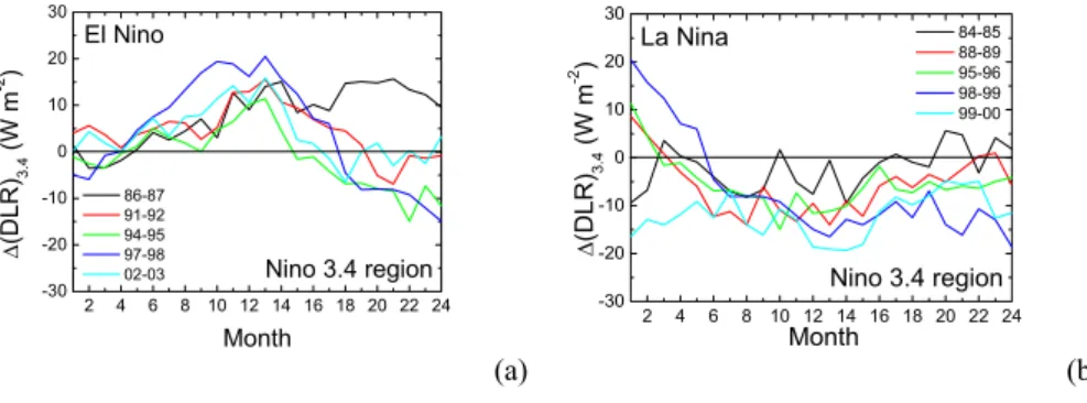
First, we investigate the evolution of each El Ni˜no or La Ni˜na event, in the representative Ni˜no-3.4 region, in order to define the time-span of the early, mature and decay phases of the phenomenon with respect to DLR. We thus calculate the mean monthly DLR in the Ni˜no-3.4 region averaged over the 11 neutral years (DLR[_{N E}3.4]), i.e. the years when no signif-icant El Ni˜no or La Ni˜na events occurred. We then defined the parameter 1(DLR)3.4=DLR_EN[3.4]−DLR[_{N E}3.4], which gives the difference between the mean monthly DLR in the Ni˜no-3.4 region (DLR[_EN3.4])for each El Ni˜no event and the average neutral year DLR (DLR[_{N E}3.4])for the same month.

In Fig. 4a, we show the time evolution of 1(DLR)3.4 for each El Ni˜no event. The same procedure is followed for the La Ni˜na events, and the corresponding plots for the individ-ual La Ni˜nas are shown in Fig. 4b. In order to facilitate the interpretation of these figures and to show clearly the begin-ning and end of an event, we present 24-month time-series.

It is evident from Fig. 4 that the maximum DLR change during warm (El Ni˜no) or cold (La Ni˜na) ENSO events oc-curs between November and January, except for the 1986– 1987 El Ni˜no, which displays a double peak behaviour (see also Wang and Fiedler, 2006), with a second maxi-mum around August 1987. Usually the highest value of

1(DLR)3.4occurs within the 3-month period from Novem-ber to January. Consequently, in our subsequent analysis we use the three month period of November, December and Jan-uary (NDJ) to study the mature phase of El Ni˜no or La Ni˜na events, August, September and October (ASO) for the earlier

(a)

(b)

(c)

Fig. 2. The distribution of net surface longwave radiation (NSL),

over tropical and subtropical Pacific for the three month pe-riod November, December, January (NDJ); (a) long-term average (1984–2004), (b) average for five El Ni˜no years, (c) average for five La Ni˜na years.

stages of ENSO development and February, March and April (FMA) for the decay phase of ENSO. Thus, in spite of the significant differences in the onset and evolution of individ-ual ENSO events, the ASO, NDJ, and FMA periods provide a frame of reference for studying in broad terms the evolution of ENSO.

(a) (b)

Fig. 3. (a): Differences in the mean downward longwave radiation (DLR), between the El Ni˜no and La Ni˜na years, over tropical and

subtropical Pacific for the period of November, December and January (NDJ), (b): The same but for NSL.

2 4 6 8 10 12 14 16 18 20 22 24 -30 -20 -10 0 10 20 30 El Nino Nino 3.4 region ∆ (D L R )3.4 (W m -2 ) Month 86-87 91-92 94-95 97-98 02-03 (a) 2 4 6 8 10 12 14 16 18 20 22 24 -30 -20 -10 0 10 20 30 Month ∆ (D L R )3.4 (W m -2 ) 84-85 88-89 95-96 98-99 99-00 Nino 3.4 region La Nina (b)

Fig. 4. DLR differences between the warm ENSO phase and neutral years; (a) in the Ni˜no-3.4 region (5 S–5 N, 170–120 W) from January of

each ENSO development to December of the following year, (b) the same but for the cold ENSO phase.

4.1 El Ni˜no events

We now define the difference DLREN–DLR, as the El Ni˜no DLR anomaly with respect to the long-term average (El Ni˜no DLR-A). This quantity gives the change in DLR during El Ni˜no years with respect to normal condition. In Fig. 5 (left side) we show the distribution of El Ni˜no DLR-A for the three month periods of ASO (top panel), NDJ (middle panel) and FMA (bottom panel), at 2.5×2.5 spatial resolution.

The DLR-A during the early stage of El Ni˜no development is around +10 Wm−2in the equatorial central Pacific and – 10 Wm−2in the western Pacific over Indonesia and Northern Australia. During the mature phase of El Ni˜no, high values of DLR-A are observed in a region confined around the equator, between 10 S–5 N that extents from the central Pacific (near the date line) to the coast of Peru. The values of the DLR-A reach about +20 Wm−2_{over most of the Ni˜no-3.4 region.} During the decay phase of El Ni˜no, values of DLR-A up to +10 Wm−2are observed roughly in the same equatorial cen-tral Pacific region as during the mature ENSO phase, but in the eastern Pacific this region now shifts north of the equator up to the south coast of Mexico (15 N). In the western Pacific DLR-A values of opposite sign are observed with values up to –10 Wm−2over the South China Sea.

In order to investigate and identify the regions that show significant changes in the DLR during El Ni˜no years with respect to the long-term values, we performed for each grid-box and for each 3-month period (ASO, NDJ, FMA) a two-tailed Student’s t-test. Our two samples are the 3-monthly DLR values for the period 1984–2004 and the correspond-ing values for the 5 years when El Ni˜no conditions prevailed. The null hypothesis is that the mean values of the two sam-ples are equal and the alternative hypothesis is that these val-ues are different. On the right-hand side of Fig. 5 we show the geographical distribution of the P-values for the ASO (top panel), NDJ (middle panel) and FMA (bottom panel). Grid-boxes with P-values smaller than 0.05 are considered to have statistically significant El Ni˜no DLR-A values. Dur-ing the mature phase of ENSO, the statistical significance of the anomalies is very high over the Ni˜no-3.4 (the small-est P-value is 0.004, observed in this region) and Ni˜no-1+2 regions (P-values less than 0.02) as well as the region be-tween them. P-values less than 0.01 are observed over two regions: a sub-region of Ni˜no-3.4, i.e. 5 N–5 S, 160–130 W and a second region in the eastern Pacific between 0–5 S and 115–90 W. There is no significant DLR signal in the west-ern Pacific during the mature phase of ENSO. On the other hand, during the early phase (ASO), the anomalies appear to

(a) (b)

(c) (d)

(e) (f)

Fig. 5. Left: The distribution at 2.5×2.5 spatial resolution of El Ni˜no DLR-A for ASO (top panel), NDJ (middle panel), and FMA (bottom

panel). Right: The distribution of P-values from a Student’s t-test.

be significant over a region in the western Pacific, over In-donesia (smallest P-value of about 0.02). The DLR change in this region precedes the appearance of significant high val-ues of DLR anomalies in the Ni˜no-3.4 region. This will be further discussed in Sect. 6. During the decay ENSO phase P-values less than 0.02 are observed over two regions: a re-gion in the central Pacific 10–0 S, 130–150 W and a rere-gion in eastern Pacific 0–10 N, 80–100 W. Further, P-values around 0.03 are found over the South China Sea.

A similar analysis was conducted for the El Ni˜no NSL anomalies (not shown here). The various parameters are de-fined in the same way as above but for NSL. The El Ni˜no NSL-A during the early stages (ASO period) of El Ni˜no de-velopment has a minimum value of about –10 Wm−2 over central and eastern Indonesia with P-value less than 0.03. In contrast, over the central Pacific the signal is not significant. During the mature phase of El Ni˜no (NDJ), the NSL-A is

around +10 Wm−2south of the equator in the central Pacific (10–0 S, 160–120 W) with P-values less than 0.02. During the decay phase (FMA) there is a NSL-A of about –10 Wm−2 over the South China Sea with P-values of about 0.02. 4.2 La Ni˜na events

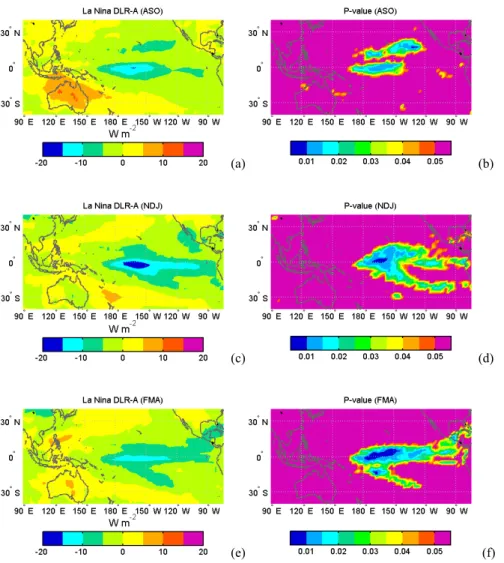
A similar analysis was conducted for the DLR anomalies dur-ing La Ni˜na events. The various parameters are defined in the same way as in Sect. 4.1, but for the La Ni˜na years. Instead of the suffix EN (El Ni˜no), we use here the suffix LN (La Ni˜na). The resulting geographical distribution of the La Ni˜na DLR anomalies (DLR-A), with respect to the long-term average, is shown on the left in Fig. 6 at the top panel for ASO, the mid-dle panel for NDJ and the bottom panel for FMA. Large neg-ative values (i.e. lower DLR for the La Ni˜na years) of about –20 Wm−2are observed in the central equatorial Pacific, in the region 2.5 S–2.5 N, 170–150 W during the mature ENSO

(a) (b)

(c) (d)

(e) (f)

Figure 6. Left: The distribution at 2.5x2.5 spatial resolution of La Niña DLR-A for ASO (top

Fig. 6. Left: The distribution at 2.5×2.5 spatial resolution of La Ni˜na DLR-A for ASO (top panel), NDJ (middle panel), and FMA (bottom

panel). Right: The distribution of P-values from a Student’s t-test.

phase (i.e. during NDJ). In the same region values of DLR-A of about –10 Wm−2are observed during both the early and decay phases of La Ni˜na.

On the right side of Fig. 6 we present the geographical distribution of P-values, which confirms that the region in the Central Pacific indicated above, displays statistically sig-nificant anomalies during all three, phases (i.e. ASO, NDJ, FMA) of La Ni˜na with P-values less than 0.02.

5 Correlation of Ni ˜no-3.4 index and DLR anomaly

The Ni˜no-3.4 index based on sea surface temperature (SST) is used extensively in recent years for identifying El Ni˜no or La Ni˜na events. The strength of the events is quantified as the three-month smoothed SST departures from normal SST, in the Ni˜no-3.4 region in the equatorial Pacific. For the same region (Ni˜no-3.4), we have calculated the 3-month smoothed anomaly of the mean monthly DLR at the surface

with respect to the average monthly DLR for the whole study period 1984–2004. This parameter will be denoted by DLR-A[3.4] and will be called “DLR-DLR-A[3.4] index”.

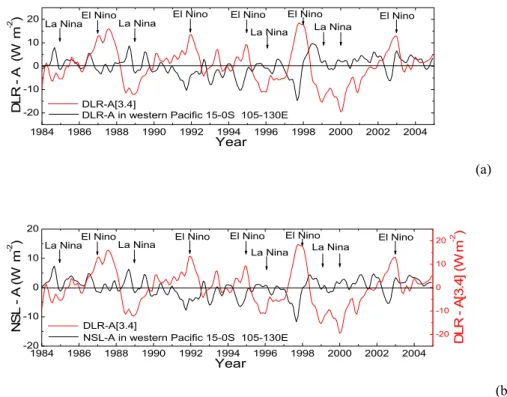
Figure 7a shows the time-series of the DLR-A[3.4] in-dex for the period 1984–2004 (black line). For compari-son we have overlaid on the same diagram the time-series of the Ni˜no-3.4 SST index (red line). The agreement be-tween the two time-series is excellent. In both time-series there are clear peaks during El Ni˜no events and minima for the La Ni˜na events. Moreover, the relative strengths of warm and cold ENSO events are very similar. DLR-A[3.4] reaches values as high as +20 Wm−2(during the strong 1997–1998 El Ni˜no), and as low as –20 Wm−2 (during the La Ni˜na of 2000–2001).

Figure 7b shows the corresponding time-series of the 3-month smoothed anomaly (NSL-A[3.4]) of the mean monthly NSL with respect to the average monthly NSL for the whole study period 1984–2004 in the Ni˜no-3.4 region.

1984 1986 1988 1990 1992 1994 1996 1998 2000 2002 2004 -30 -20 -10 0 10 20 30 -4 -2 0 2 4 El Nino N in o -3 .4 i n d e x ( o C ) La Nina La Nina La Nina El Nino El Nino El Nino Nino-3.4 region 5S-5N 170-120W El Nino La Nina Year D L R A [3 .4 ] ( W m -2 ) (a) 1984 1986 1988 1990 1992 1994 1996 1998 2000 2002 2004 -15 -10 -5 0 5 10 15 -4 -2 0 2 4 Nino-3.4 region 5S-5N 170-120W El Nino El Nino El Nino El Nino El Nino La Nina La Nina La Nina La Nina N S L A [3 .4 ] (W m -2 ) Year N in o -3 .4 i n d e x ( o C ) (b)

Fig. 7. Time-series of downward longwave radiation (DLR-A[3.4]), and net downwelling longwave radiation at the surface (NSL-A[3.4])

anomaly (defined with respect to the average monthly DLR for the whole study period 1984–2004) in the Ni˜no-3.4 region (black line). Overlaid is the time-series of the Ni˜no-3.4 index (red line).

The NSL-A[3.4] shows lower variability than the DLR-A[3.4] but this is at least partly due to the fact that the region of the most significant NSL changes during the ENSO lies to the south of the Ni˜no-3.4 region (see Fig. 3b).

Linear regression between DLR-A[3.4] and the Ni˜no-3.4 index yielded a correlation coefficient of r=0.91 and a slope of 7.7±0.2 Wm−2/oC , as shown in Fig. 8a. The correspond-ing plot for NSL-A[3.4] vs. the Ni˜no-3.4 index is shown in Fig. 8b. The correlation coefficient is 0.51 and the slope equals 2.0±0.2 Wm−2/◦C. These values show that during El Ni˜no conditions in the Ni˜no-3.4 region, the DLR increases at a higher rate than the longwave emission from the surface due to the increase in the sea surface temperature. Thus the NSL in the Ni˜no-3.4 region increases during the warm phase of ENSO by roughly 2 Wm−2_{for a 1 degree increase in SST.} This is consistent with the term “super greenhouse effect” (Ramanathan and Collins 1991; Inamdar and Ramanathan 1994) whereby the trapping of longwave radiation in the at-mosphere increases faster than the longwave emission from the Earth’s surface as the temperature increases.

In Fig. 9a we show the geographical distribution of the correlation coefficient given by linear regression of the time-series of DLR-A in each 2.5×2.5 degree grid-box and the Ni˜no-3.4 index time-series. The maximum values of the cor-relation coefficient are observed, expectedly, in the Ni˜no-3.4 region itself although there are values higher than 0.5 all over the central and eastern Pacific. In the western Pacific there is

an anti-correlation between the DLR-A and Ni˜no-3.4 index time-series, although in absolute terms the correlation coef-ficients are not as high as in the eastern Pacific.

In Fig. 9b, we also show the distribution of the correlation coefficient given by linear regression of the time-series of NSL-A in each 2.5×2.5 degree grid-box and the Ni˜no-3.4 index time-series. The maximum values of the correlation coefficient here do not exceed 0.7 and they are observed over a smaller region, to the south of the Ni˜no-3.4 region, at (0– 10 S, 160–140 W).

6 Time lag between western and eastern Pacific DLR

Anomalies

There is a region in the western Pacific (central Indonesia) which displays significant anomalies during the early phase (ASO) of ENSO development. The DLR anomalies in this region seem to precede the appearance of significant anoma-lies in the Ni˜no-3.4 region. In order to further investigate this, we have produced correlation coefficients for each 2.5×2.5 grid-box, between the time-series of the DLR-A in each pixel and the time-series of the DLR-A[3.4] index, after intro-ducing in the latter a time shift of –1, –2 , . . . , –8 months. We constructed geographical distributions of the correlation coefficients, and compared them against the map with zero time lag (Fig. 9a). In all cases but one, the correlation

-3 -2 -1 0 1 2 3 -30 -20 -10 0 10 20 30 Nino-3.4 region r = 0.91 D L R - A[ 3 .4 ] (W m -2 ) Nino-3.4 index (oC) slope = 7.7±0.2Wm-2_/ o_C (a) -3 -2 -1 0 1 2 3 -20 -10 0 10 20 Nino-3.4 region r = 0.51 slope = 2.0±0.2Wm-2/ oC Nino-3.4 index (oC) N SL - A[ 3 .4 ] (W m -2 ) (b)

Fig. 8. (a) Scatter plot between the DLR-A[3.4] and the Ni˜no-3.4 index, (b) between the NSL-A[3.4] and the Ni˜no-3.4 index.

(a) (b)

Fig. 9. Geographical distribution of correlation coefficient between, (a) DLR-A and the Ni˜no-3.4 index, (b) NSL-A and Ni˜no-3.4 index.

deteriorated over the entire area. The one exception is shown in the map of the 3-month shift (Fig. 10a). There is a region in the western Pacific, north of Australia (central Indone-sia), indicated by a rectangle (0–15 S, 105–130 E), where the (anti)correlation improves, and takes its highest abso-lute value when the time-series of the DLR-A[3.4] index is shifted by –3 months. The maximum value of the correlation coefficient increases in absolute value from 0.42 with no time shift, to 0.57 with a 3-month time shift.

We have, subsequently, calculated the correlation coeffi-cient between the average DLR-A in the western Pacific rect-angle shown in Fig. 10a and the DLR-A[3.4] index shifted by 0, –1, .., –8 months. In Fig. 10b we have plotted the value of this correlation coefficient (the values are negative, because the two DLR anomalies are anti-correlated) as a function of the time lag introduced (in months). It is again obvious that highest anti-correlation is observed when the DLR-A[3.4] in-dex time-series is shifted by –3 to –4 months. This means that DLR anomalies in the western Pacific rectangle precede the anomalies in the Ni˜no-3.4 region by 3–4 months. The significance of the western Pacific for initializing El Ni˜no has already been noted by Wang (2002) who found that the 850-mb zonal wind anomalies in the western Pacific region with coordinates 5 S–5 N, 120–170 E lead the Ni˜no-3 SST anomalies by 4 months (note the overlap of our western Pa-cific region with that of Wang 2002).

In Fig. 11a, we show the mean DLR-A time-series in the western Pacific rectangle (black line). For comparison we have overlaid on the same diagram the DLR-A[3.4] index time-series (red line). It is clear that the DLR-A in the west-ern Pacific shows a minimum before the peak of the DLR-A[3.4] index for each El Ni˜no. The minimum value of the DLR-A in the western Pacific is about –15 Wm−2before the intense 1997–1998 El Ni˜no.

In Fig. 11b, we also show the mean NSL-A time-series in our western Pacific rectangle (black line) and the DLR-A[3.4] index time-series (red line). The behaviour of the NSL-A time-series in the western Pacific rectangle is very similar to that of DLR-A, although the variability is much lower.

7 Effects of total precipitable water and cloud amount

variability on DLR during ENSO

The air temperature and the water vapour content of the at-mosphere, especially of the lower atmospheric layer, play the most important role in determining the DLR reaching the Earth’s surface, followed in order of significance by the cloud amount of low, middle and high cloud, respectively (Pavlakis et al., 2004).

The time-series of the anomaly of the mean monthly DLR in the Ni˜no-3.4 region (DLR-A [3.4] index) with respect to the average monthly DLR for the entire study period

(a) 0 1 2 3 4 5 6 7 -0,5 -0,4 -0,3 -0,2 C o rr e la ti o n o f D L R A in N in o -3 .4 re g io n a n d w e st e rn Pa ci fi c Month shift (b)

Fig. 10. (a) Geographical distribution of correlation between the DLR-A and the DLR-A[3.4] in the Ni˜no-3.4 region with a 3-month shift, (b) correlation coefficient of the DLR-A in the western Pacific and the DLR-A[3.4] as a function of the number of months shift of the

DLR-A[3.4]. 1984 1986 1988 1990 1992 1994 1996 1998 2000 2002 2004 -20 -10 0 10 20

DLR-A in western Pacific 15-0S 105-130E

El Nino El Nino El Nino El Nino El Nino La Nina La Nina La Nina La Nina Year D L R - A (W m -2 ) DLR-A[3.4] (a) 1984 1986 1988 1990 1992 1994 1996 1998 2000 2002 2004 -20 -10 0 10 20 -20 -10 0 10 20 D L R - A [3 .4 ] (W m -2 )

NSL-A in western Pacific 15-0S 105-130E

El Nino El Nino El Nino El Nino El Nino La Nina La Nina La Nina La Nina Year N S L - A (W m -2 ) DLR-A[3.4] (b)

Figure 11. Downward longwave radiation (DLR), and net downwelling longwave radiation at

Fig. 11. Downward longwave radiation (DLR), and net downwelling longwave radiation at the surface (NSL) anomaly time series in the

western Pacific region 15 S–15 N, 120–140 E (black line) compared with DLR anomaly in Ni˜no-3.4 region (red line).

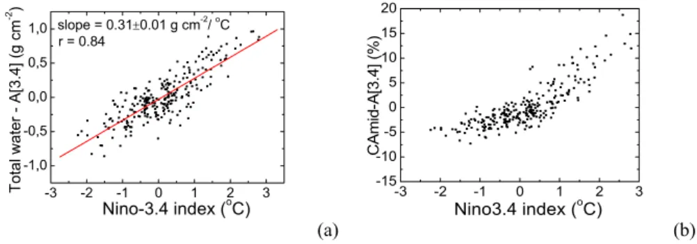
1984–2004, shows an excellent correlation with the Ni˜no-3.4 index. This is due to the fact that the Ni˜no-Ni˜no-3.4 index is based on sea surface temperature (SST) which is linked to the water vapour content of the atmosphere. We calcu-lated the anomaly of the mean monthly total column wa-ter vapour with respect to the average monthly total col-umn water vapour from the NCEP/NCAR database for the whole study period 1984–2004 in the Ni˜no-3.4 region (Total water–A[3.4]). Linear regression between the Total water– A[3.4] and the Ni˜no-3.4 index yielded a correlation coeffi-cient of 0.84 and a slope of 0.31±0.01 g cm−2/◦C, as shown in Fig. 12a.

We also calculated the anomaly of the mean monthly low, middle and high-level cloud amount with respect to the cor-responding values, for the whole study period 1984–2004 in the Ni˜no-3.4 region. We then created scatter plots between these anomalies and the Ni˜no-3.4 index. We found no corre-lation between the low cloud amount anomaly and the Ni˜no-3.4 index (correlation coefficient r=0.1). We note that there are uncertainties in ISCCP low cloud amount because from the satellite point of view low clouds under optically thick middle or high level clouds are not observed. Linear regres-sion between the middle and high cloud amount anomalies and the Ni˜no-3.4 index yielded a correlation coefficient of

-3 -2 -1 0 1 2 3 -1,0 -0,5 0,0 0,5 1,0 slope = 0.31±0.01 g cm-2/ o_C r = 0.84 Nino-3.4 index (oC) T o ta l w a te r - A[ 3 .4 ] (g cm -2 ) (a) -3 -2 -1 0 1 2 3 -15 -10 -5 0 5 10 15 20 C Ami d -A[ 3 .4 ] (% ) Nino3.4 index (oC) (b)

Figure 12. (a) Scatter plot between the total column water vapour anomaly in the Niño-3.4

Fig. 12. (a) Scatter plot between the total column water vapour anomaly in the Ni˜no-3.4 region and the Ni˜no-3.4 index, (b) scatter plot

between the middle cloud amount anomaly in the Ni˜no-3.4 region and the Ni˜no-3.4 index.

0.83 and 0.77, respectively. In Fig. 12b we show, as an ex-ample, the scatter plot of the middle cloud amount anomaly (CAmid–A[3.4]) versus the Ni˜no-3.4 index. However, in the tropics the middle and high clouds only marginally influ-ence the DLR owing to the high moisture in the lower part of the atmosphere (Tian and Ramanathan, 2002). This is verified by inspection of the scatter plot between CAmid– A[3.4] and Ni˜no-3.4 index (Fig. 12b). The slope in the scat-ter plot becomes steeper for values of Ni˜no-3.4 index greascat-ter than 1.5◦C. The same is true for the scatter plot between high cloud amount anomaly and Ni˜no-3.4 index (not shown here). The steeper slope in these scatter plots is indicative of the onset of deep convection in the region (Ramanathan and Collins 1991). The onset of deep convection however does not change the rate of increase of the DLR-A[3.4] for SST anomalies greater than 1.5◦C (Fig. 8). In contrast other radi-ation variables crucial for the development of an ENSO event such as the downward shortwave radiation (DSR) at the sur-face or the longwave radiation absorbed by the atmosphere in the Ni˜no-3.4 region are affected by the onset of deep con-vection.

The time-series of the mean monthly DLR anomaly (DLR-A) in the region north of Australia (15 S–0 S, 105 E–130 E), exhibits an anti-correlation with the DLR-A [3.4] time-series and precedes it by 3–4 months. We have found that only the time-series of total water vapour anomaly (Total water–A) leads the DLR-A [3.4] time-series by 3–4 months in contrast with the time-series of the other parameters that influence the DLR. Linear regression between the Total water–A and the DLR-A [3.4] index yielded a correlation coefficient of –0.52 (anticorrelation). When the DLR-A[3.4] index was shifted by –3 months the highest anti-correlation is observed, with a value of –0.64. The reduction of atmospheric water vapour in the western Pacific over the region of central Indonesia is in agreement with the reduction of precipitation over the same region that preceded the 1997/1998 El Ni˜no, as observed by Curtis et al. (2001). We found no correlation between the low-level cloud amount anomaly and the DLR-A[3.4] index but this may be due to uncertainties in the ISCCP data.

8 Conclusions

To summarize, our model calculations, which are based on ISCCP-D2 cloud climatologies, and temperature and humid-ity profile information from NCEP/NCAR reanalysis, show a high variability in the downward longwave radiation (DLR) at the surface of the Earth and the net downwelling longwave radiation at the surface (NSL) over the tropical and subtrop-ical Pacific Ocean during ENSO events. We have found that the enhancement of DLR during warm ENSO phases, com-pared with neutral years, is not confined to the Ni˜no-3.4 re-gion but extents over a much broader area in the central and eastern Pacific. This enhancement of DLR (DLR-A), for the three month period NDJ, is more than +10 Wm−2, in a broad swath in the central Pacific extending to the coast of South America. A maximum DLR-A, of about 20 Wm−2, is ob-served within the Ni˜no-3.4 region.

During the cold phases of ENSO, values of DLR-A less than –10 Wm−2 are observed in a small sub-region of the Ni˜no-3.4 region (2.5 S–2.5 N, 170–150 W), for both ASO and FMA periods. Minimum values of DLR-A, of about – 20 Wm−2, are observed in the central Pacific near the date-line and within the Ni˜no-3.4 region for the NDJ period, but in a more confined region compared with the corresponding values during the ENSO warm phases.

The absolute value of NSL shows less variability com-pared with DLR. The highest values of the enhancement of NSL during warm ENSO phases compared with cold ENSO phases, appear south of the Ni˜no-3 and Ni˜no-3.4 regions and are about 15 Wm−2.

The Ni˜no-3.4 index is very often used to define the phase and strength of ENSO events. We calculated the correlation coefficient given by linear regression of the time-series of the monthly DLR anomaly, referenced to the whole study period 1984–2004, in each 2.5×2.5 degree grid-box and the Ni˜no-3.4 index, and found values higher than 0.5 over the central and eastern tropical Pacific. Values higher than 0.85 are observed in the Ni˜no-3.4 region. Thus, the average DLR anomaly in the Ni˜no-3.4 region (DLR-A [3.4] index), is a very useful index to describe and study ENSO events and

can be used to asses whether or not El Ni˜no or La Ni˜na con-ditions prevail. It is important to note that DLR is an easily measurable quantity using a pyrgeometer and contains infor-mation both for oceanic (i.e. SST) and atmospheric (i.e. wa-ter vapour) processes.

We further investigated the DLR anomaly time-series in the western Pacific using the DLR-A [3.4] index time-series as our reference. We found a significant anti-correlation be-tween the two time-series over the ocean north of Australia up to the equator. There is a region in the western Pacific over Indonesia and western Java (15–0 S, 105–130 E) where the DLR anomaly leads the corresponding anomaly in the Ni˜no-3.4 region by 3–4 months. Thus, DLR measurements in this region will be very useful for the study of the time evolution of El Ni˜no events.

Acknowledgements. The ISCCP-D2 data were obtained from the

NASA Langley Research Center (LaRC) Atmospheric Sciences Data Center (ASDC). The NCEP/NCAR Global Reanalysis Project data were obtained from the National Oceanic and Atmospheric Administration (NOAA) Cooperative Institute for Research in Environmental Sciences (CIRES) Climate Diagnostics Center, Boulder, Colorado, USA.

Edited by: W. Conant

References

Bjerknes, J.: A possible response of the atmospheric Hadley circu-lation to equatorial anomalies of ocean temperature, Tellus, 18, 820–829, 1966.

Bjerknes, J.: Atmospheric teleconnections from the equatorial Pa-cific, Mon. Wea. Rev., 97, 163–172, 1969.

Cane, M. A., Matthias, M., and Zebiak, S. E.: A study of self ex-cited oscillations of the tropical ocean–atmosphere system. Part I: Linear analysis, J. Atmos. Sci., 47, 1562–1577, 1990. Chou, Shu-Hsien, Chou, Ming-Dah, Chan, Pui-King, Lin,

Po-Hsiung, and Wang, Kung-Hwa: Tropical warm pool surface heat budgets and temperature: Contrasts between 1997/98 El Ni˜no and 1998/99 La Ni˜na, J. Climate, 17, 1845–1858, 2004. Curtis, S. and Adler, R.: ENSO indices Based on patterns of

satellite-derived precipitation, J. Climate, 13, 278–2793, 2000. Curtis, S., Adler, R., Huffman, G., Nelkin, E., and Bolvin, D.:

Evo-lution of tropical and extratropical precipitation anomalies dur-ing the 1997–1999 ENSO cycle, Int. J. Climatol., 21, 961–971, 2001.

Dijkstra, H. A.: The ENSO phenomenon: theory and mechanisms, Adv. Geosci., 6, 3–15, 2006,

http://www.adv-geosci.net/6/3/2006/.

Fedorov, A. V., Harper, S. L., Philander, S. G., Winter, B., and Wit-tenberg, A.: How predictable is El Ni˜no?, BAMS 84, 911–919, 2003.

Hanley, D. E., Bourassa, M. A., O’Brien, J. J., Smith, S. R., and Spade, E. R.: A quantitative evaluation of ENSO Indices, J. Cli-mate, 16, 1249–1258, 2003.

Harrison, M. J., Rosati, A., Soden, B. J., Galanti, E., and Tziper-man, E.: An evaluation of Air-Sea flux products for ENSO sim-ulation and prediction, Mon. Wea. Rev., 130, 723–732, 2002.

Hatzianastassiou, N., Croke, B., Kortsalioudakis, N., Vardavas, I., and Koutoulaki, K.: A model for the longwave radiation budget of the NH: Comparison with Earth Radiation Budget Experiment data, J. Geophys. Res., 104, 9489–9500, 1999.

Hatzianastassiou, N. and Vardavas, I.: Shortwave radiation budget of the Southern Hemisphere using ISCCP C2 and NCEP/NCAR climatological data, J. Climate, 14, 4319–4329, 2001.

Inamdar, A. K. and Ramanathan V.: Physics of greenhouse effect and convection in warm oceans, J. Climate, 7, 715–731, 1994. IPCC, 2001: Climate Change: The Scientific Basis. Contribution of

Working Group I to the Third Assessment Report of the Inter-governmental Panel on Climate Change, edited by: Houghton, J. T., Ding, Y., Griggs, D. J., Noguer, M., van der Linden, P. J., Dai, X., Maskell, K., and Johnson, C. A., Cambridge University Press, Cambridge, United Kingdom and New York, NY, USA, 2001.

Jin, F. F.: An equatorial ocean recharge paradigm for ENSO. Part I: Conceptual model, J. Atmos. Sci., 54, 811–829, 1997a. Jin, F. F.: An equatorial ocean recharge paradigm for ENSO. Part

II: A stripped-down coupled model, J. Atmos. Sci., 54, 830–847, 1997b.

Kistler, R., Kalnay, E., Collins, W., Saha, S., White, G., Woollen J., Chelliah, M., Ebisuzaki, W., Kanamitsu, M., Kousky, V., van den Dool, H., Jenne, R., and Fiorino, M.: The NCEP-NCAR 50-Year Reanalysis: Monthly Means CD ROM and Documentation, Bull. Am. Meteorol. Soc., 82, 247–268, 2001.

McCreary, J. P. and Anderson, D. L. T.: An overview of coupled ocean–atmosphere models of El Ni˜no and the Southern Oscilla-tion, J. Geophys. Res., 96, 3125–3150, 1991.

McPhaden, M. J., Busalacchi, A. J., Cheney, R., et al.: The trop-ical ocean-global atmosphere observing system: A decade of progress, J. Geophys. Res., 103, 14 169–14 240 1998.

Matsoukas, C., Banks, A. C., Hatzianastassiou, N., Pavlakis, K. G., Hatzidimitriou, D., Drakakis, E., Stackhouse, P. W., and Var-davas, I.: Seasonal heat budget of the Mediterranean Sea, J. Geo-phys. Res., 110, C12008, doi:10.1029/2004JC002566, 2005. Neelin, J. D., Battisti, D. S., Hirst, A. C., Jin, F. F., Wakata, Y.,

Yamagata, T., and Zebiak, S. E.: ENSO theory, J. Geophys. Res., 103, 14 262–14 290, 1998.

Pavlakis, K. G., Hatzidimitriou, D., Matsoukas, C., Drakakis, E., Hatzianastassiou, N., and Vardavas, I.: Ten-year global distribu-tion of downwelling longwave radiadistribu-tion, Atmos. Chem. Phys., 4, 127–142, 2004,

http://www.atmos-chem-phys.net/4/127/2004/.

Philander, S. G.: El Ni˜no, La Ni˜na, and the Southern Oscillation, Academic Press, San Diego, CA , 1–289, 1990.

Picaut, J., Masia, F., and du Penhoat, Y.: An advective–reflective conceptual model for the oscillatory nature of the ENSO, Sci-ence, 277, 663–666, 1997.

Ramanathan, V. and Collins, W.: Thermodynamic regulation of ocean warming by cirrus clouds deduced from observations of the 1987 El Ni˜no, Nature, 351, 27–32, 1991.

Rossow, W. B. and Schiffer, R. A.: Advances in understanding clouds from ISCCP, Bull. Am. Meteorol. Soc., 80, 2261–2288, 1999.

Suarez, M. J. and Schopf, P. S.: A delayed action oscillator for ENSO, J. Atmos. Sci., 45, 3283–3287, 1988.

Tian, B. and Ramanathan, V.: Role of tropical clouds in surface and atmospheric energy budget, J. Climate, 15, 296–305, 2002.

Trenberth, K. E.: The Definition of El Ni˜no, Bull. Amer. Meteorol. Soc., 78, 2771–2777, 1997.

Trenberth, K. E. and Stepaniak, D. P.: Indices of El Ni˜no evolution, J. Climate, 14, 1697–1701, 2001.

Vardavas, I. and Carver, J. H.: Solar and terrestrial parameteri-zations for radiative convective models, Planet. Space Sci., 32, 1307–1325, 1984.

Wolter, K. and Timlin, M. S. : Measuring the strength of ENSO events: How does 1997/98 rank?, Weather, 53, 315–324, 1998.

Wang, C., Weisberg, R. H., and Virmani, J. I.: Western Pacific in-terannual variability associated with the El Ni˜no–Southern Os-cillation, J. Geophys. Res., 104, 5131–5149, 1999.

Wang, C.: A unified oscillator model for the El Ni˜no–Southern Os-cillation, J. Climate, 14, 98–115, 2001.

Wang, C.: Atmospheric circulation cells associated with the El Ni˜no–Southern Oscillation, J. Climate, 15, 399–419, 2002. Wang, C. and Fiedler P. C.: ENSO variability and the Eastern

Trop-ical Pacific: A Review, Progress in Oceanography, 69, 239–266, 2006.