HAL Id: hal-00463239
https://hal.archives-ouvertes.fr/hal-00463239
Submitted on 18 Apr 2021
HAL is a multi-disciplinary open access
archive for the deposit and dissemination of
sci-entific research documents, whether they are
pub-lished or not. The documents may come from
teaching and research institutions in France or
abroad, or from public or private research centers.
L’archive ouverte pluridisciplinaire HAL, est
destinée au dépôt et à la diffusion de documents
scientifiques de niveau recherche, publiés ou non,
émanant des établissements d’enseignement et de
recherche français ou étrangers, des laboratoires
publics ou privés.
Distributed under a Creative Commons Attribution| 4.0 International License
Generalized composition law from 2x2 matrices
R. Giust, J.-M. Vigoureux, J. Lages
To cite this version:
R. Giust, J.-M. Vigoureux, J. Lages.
Generalized composition law from 2x2 matrices.
Amer-ican Journal of Physics, AmerAmer-ican Association of Physics Teachers, 2009, 77 (11), pp.1068-1073.
�10.1119/1.3152955�. �hal-00463239�
Generalized composition law from 2 Ã 2 matrices
R. Giusta兲Institut FEMTO-ST, UMR CNRS 6174, Université de Franche-Comté, 16 Route de Gray, 25030 Besançon Cedex, France
J.-M. Vigoureuxb兲 and J. Lagesc兲
Institut UTINAM, UMR CNRS 6213, Université de Franche-Comté, 16 Route de Gray, 25030 Besançon Cedex, France
Many results that are difficult can be found more easily by using a generalization in the complex plane of Einstein’s addition law of parallel velocities. Such a generalization is a natural way to add quantities that are limited to bounded values. We show how this generalization directly provides phase factors such as the Wigner angle in special relativity and how this generalization is related in the simplest case to the composition of 2⫻2 S-matrices.
I. INTRODUCTION
In special relativity the composition law of parallel veloci-ties appears to be the natural addition law for quantiveloci-ties whose values are limited to the closed interval关⫺1,1兴, where we have set the speed of light c = 1. It is natural to generalize the composition law of parallel velocities to the complex plane as
A= A2丣A1=
A1+ A2 1 + A2A1
, 共1兲
where A1 and A2 are complex quantities and where the de-nominator appears as a normalization term共if not otherwise stated, A¯ denotes the complex conjugation operation兲. The physical meaning of this composition law is similar to that of the composition law of parallel velocities in special relativ-ity. Equation 共1兲 shows that no matter what real values we give to A1= v1 and A2= v2, subject only to v1⬍ c and v2⬍ c, the value of the resulting velocity A = w cannot exceed the speed of light c = 1. In the same way, no matter the values of the complex quantities A1 and A2 共subject only to 兩A1兩⬍1 and兩A2兩⬍1兲, the modulus of the resulting quantity A cannot exceed unity.
Because it avoids infinities, such a generalization of Ein-stein’s composition law of velocities appears to be a natural addition law in a closed interval. As expected, it reduces to the usual addition of arithmetics when the quantities are small. As shown in Refs. 1–3, the use of this composition law quickly leads to important theoretical results and pro-vides useful algorithms for computer calculations. The use of Eq.共1兲 also leads to results that converge more rapidly than by using transfer matrices.4
II. SOME SIMPLE EXAMPLES
We consider three examples1–3where the use of Eq.共1兲is useful. The examples are the composition of two nonparallel velocities in special relativity, the reflection coefficient of a Fabry–Pérot in optics, and the characteristics of a polarizer resulting from the association of two successive nonperfect polarizers.
The composition law for two parallel velocities v1and v2 in special relativity is共c=1兲
w= v2丣v1= v1+ v2
1 + v1v2
. 共2兲
The calculation of the resulting velocity of two parallel ve-locities is straightforward. However, it is not when the two velocities are not parallel for which calculations may be te-dious. They become simple when we consider Eq.共1兲, which is the generalization in the complex plane of Eq. 共2兲. As explained in Ref.1, we replace each velocity vជiby the
com-plex number,
Vi= tanhai 2e
i␣i, 共3兲
where the rapidity ai is related to the modulus of vជi by
tanh ai= vi and where phase ␣i gives the orientation of vជi
with respect to an arbitrary axis of the reference frame of the observer in the plane of vជ and v1 ជ. The modulus and phase2 ␣ of the velocity wជ resulting from the relativistic composition of vជ and v1 ជ are directly obtained2
1 by using Eq.共1兲, W= tanha 2e i␣ = V2丣V1= tanha1 2e i␣1 + tanha2 2e i␣2 1 + tanha2 2e −i␣2 tanha1 2e i␣1 . 共4兲 The modulus and the phase of Eq. 共4兲 give respectively the magnitude of the resulting velocity wជ 共because w=tanh a兲 and specify the direction␣ of wជ in the plane共vជ ,v1 ជ兲.2
In optics the overall reflection coefficient of a Fabry–Pérot interferometer can be obtained by taking into account all virtual paths of light inside the interferometer.2 The total probability amplitude for light to be reflected by the system can also be directly obtained共for any number of interfaces兲 by using Eq.共1兲. Here
Ri= rie
ii 共5兲
is the complex reflection coefficient of an incident wave on interface i, where riis the Fresnel coefficient of that interface
andiis the phase shift corresponding to the propagation of
light through the same homogeneous layer between two suc-cessive interfaces. For two interfaces the reflection coeffi-cient of the whole system can be obtained directly by using law共1兲,
R= rei= R 2丣R1= r1ei1+ r 2ei2 1 + r2e−i2r1ei1 . 共6兲
Again, the modulus and the phase of Eq.共6兲give the overall reflection coefficient and phase of the reflected wave.
Similarly, we can consider the composition of two nonper-fect polarizers P1and P2.
3
The polarizer P resulting from the combination of polarizers P1and P2共in that order兲 can also be obtained from Eq. 共1兲. As explained in Ref. 3, each po-larizer is characterized by Pi= tanh ␥i 2e i␣i , 共7兲
where ␥i is the quality of the polarizer and ␣i gives the
orientation of the polarizer axis with respect to an arbitrary reference axis. Typically,␥i= ⌫iz, where ⌫iis the differential
absorption rate of the polarizer and z is the distance traveled by the light wave inside the polarizer. The case of a perfect polarizer5 corresponds to ␥i→ +⬁. The polarizer’s
orienta-tions and the reference axis are coplanar. The characteristics of the resulting polarizer P are given by3
P= tanh␥ 2e i␣ = P2丣P1= tanh␥1 2 e i␣1 + tanh␥2 2e i␣2 1 + tanh␥1 2e −i␣1 tanh␥2 2e i␣2 . 共8兲 By using the composition law 共8兲 we easily extract the ␥
factor and its direction␣.
The use of the composition law共1兲 is general and can be applied to any number of coplanar velocities in special rela-tivity, to any number of interfaces for the case of multilayers, and to any number of successive polarizers. In such cases we have to iterate Eq.共1兲as relation2,3,6
A= An丣共An−1丣 ¯ 共A2丣A1兲兲. 共9兲
The successive iteration of Eq. 共1兲yields the desired result. Equation 共9兲 leads to algorithms that are useful for many problems. It is easy to compute A2丣A1and then to compose the result with A3and so on.
As explained in Refs.7and2, the expression for A in Eq.
共9兲 can be written down directly by using a complex gener-alization of the elementary symmetric functions of the vari-ables A1, A2, . . . , An, which are extensively used in the theory
of polynomials.8,9
Our aim in this paper is to show how Eq.共1兲is related to 2 ⫻ 2 matrices and how it provides a simple way to calculate the four elements of scattering matrices 共S-matrices兲. We also show how the use of Eq.共1兲leads naturally to a particu-lar phase, which for the case of the special relativity is re-lated to the Thomas precession.
III. MATRIX REPRESENTATION
We now explain how the composition law共1兲is related to 2 ⫻ 2 matrices.
A. Mathematical definitions
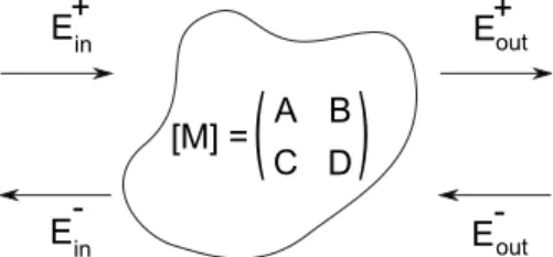
Consider a physical system 共see Fig. 1兲 in which two physical quantities共the inputs兲 Ein
+ and Ein
−
are linearly related
to two other physical quantities 共the outputs兲, Eout +
and Eout −
. These relations can be written as a 2 ⫻ 2 matrix as
冉
Ein + Ein−冊
=冉
A B C D冊
冉
Eout + Eout−冊
. 共10兲This general representation is, for example, used to describe a birefringent system with the help of Jones matrices 共see, for example, Ref.3兲, or to estimate properties of a multilayer stack with the Abeles matrices.10It is possible to define using the 2 ⫻ 2 matrix in Eq. 共10兲, hereafter called 关M兴, the four coefficients R+, R−, T+, and T−共this notation is chosen in analogy to the classical reflection and transmission coeffi-cients of a multilayer device兲,
R+=
冏
Ein − Ein+冏
E out − =0 =C A, 共11a兲 R−=冏
Eout + Eout−冏
E in +=0 = −B A, 共11b兲 T+ =冏
Eout + Ein+冏
E out − =0 = 1 A, 共11c兲 T−=冏
Ein − Eout−冏
E in +=0 =det关M兴 A . 共11d兲We introduce the variable ⌰ defined by ⌰ =D
A. 共12兲
If we use Eqs.共11兲and共12兲, it is easy to verify that T+T−
− R+R−
= ⌰, 共13兲
which constitutes a generalization of the Stokes relation, which is well known in the optics of multilayer devices共see, for example, Ref. 12兲. We also introduce the conjugation operation共denoted by the bar兲,
R+ = − R−=B A 共14a兲 and R− = − R+. 共14b兲
The conjugation operation does not necessarily correspond to the usual complex conjugation 关compare Eqs. 共11a兲 and
共14a兲兴. For Hermitian matrices the correspondence does hold.
With these definitions the关M兴-matrix can be written as Fig. 1. Schematic representation of the linear relations between input and output quantities.
关M兴 =T1+
冉
1 R+ R+
⌰
冊
. 共15兲This form of关M兴 will be useful in the following derivations.
B. Composition laws of the R and T variables
We now focus on the properties of the four coefficients R21+, R21−, T21+, and T21− of a system characterized by its 关M21兴-matrix, resulting from the composition of two sub-systems characterized by the two 关M1兴- and 关M2兴-matrices defined by 关M1兴 = 1 T1+
冉
1 R1+ R1+ ⌰1冊
and 关M2兴 = 1 T2+冉
1 R2+ R2+ ⌰2冊
. 共16兲 The关M21兴-matrix is the result of the product of two matrices: 关M21兴=关M2兴关M1兴. Equations 共12兲–共14兲 allow us to express the composition laws for R21+ , T21 + , R21 − , and T21 − as R21+ = R2+丣R1+= R 1 + ⌰2+ R2 + 1 + R1 +R 2 + , 共17a兲 R21− = R2−丣R1−= R1−+ R2−⌰1 1 + R1 −R 2 − , 共17b兲 T 21 + = T2 +丢T 1 + = T1+T2+ 1 + R1 +R 2 +, 共17c兲 T21− = T2−丢T1−= T 1 −T 2 − 1 + R1 −R 2 −. 共17d兲
Equation共14兲can be used to show that the denominators in Eq.共17兲are the same, 1 + R1
+R 2 + = 1 + R1 −R 2 − .
C. Composition law of the ⌰ variables
Although the ⌰ variable has been introduced in an ad hoc way in Eq.共12兲, it is interesting to find its composition law. We consider two processes characterized by the two vari-ables ⌰1 and ⌰2. If we start from the generalized Stokes relation共13兲and use Eq.共17兲, we find
⌰21= T21 +T 21 − − R21 +R 21 − 共18a兲 = T1+T2+T1−T2−−关R+1⌰2+ R2+兴关R1−+ R2−⌰1兴 关1 + R1 +R 2 +兴2 . 共18b兲
From Eq. 共13兲 we know that T1 +T 1 − = ⌰1+ R1 +R 1 − and T 2 +T 2 − = ⌰2+ R2 +R 2 −
. Consequently Eq.共18b兲 becomes ⌰21= ⌰1⌰2+ R1 +R 2 + 1 + R1 +R 2 + . 共19兲
This expression can be considered as the composition law for ⌰1 and ⌰2. In Sec. IV we will give the meaning of ⌰ for various physical contexts.
D. S-matrix
By definition, the four coefficients R+, T+, R−, and T− are the four elements of the S-matrix associated with scatter-ing,
S=
冉
R+ T−
T+ R−
冊
. 共20兲Equation共17兲shows that the composition of two S-matrices can be written as S= S2ⴰ S1=
冉
R2+丣R1+ T2−丢T1− T 2 +丢T 1 + R 2 −丣R 1 −冊
. 共21兲The use of the composition laws丣 and丢gives the elements of the S-matrix without resorting to the usual transfer matri-ces.
IV. THE ⌰ PHASE FACTOR
We now consider conservative systems described by the unitary matrix关U兴. In this context the ⌰ variables are modu-lus one complex numbers of the form ei. Our aim is to show
that the phases associated with the physical modes E+and E− in Eq.共10兲can be written as a sum of phases when the two modes are not coupled, plus a phase that is simply expressed with the help of the 丣 law.
A. The composition law in the case of unitary matrices
The general expression of a 2 ⫻ 2 unitary matrix is 关U兴 =
冉
cos eiu
− sin eiv sin e−iv cos e−iu
冊
ei
, 共22兲
where, , u, and v are real numbers. The overall phase
can be omitted without loss of generality and hereafter we set it equal to zero. As we can see, when the modes are not coupled, that is, when = 0, the evolution matrix reduces to the simple diagonal expression,
关U=0兴 = 关u兴 =
冉
eiu 0
0 e−iu
冊
. 共23兲The phase difference between the uncoupled modes E+ and
E−is equal to 2u. When ⫽ 0, the evolution of the modes are coupled and the关U兴-matrix can be factorized as
关U兴 = 关U=0兴关M兴 = 关u兴关M兴 共24a兲
=
冉
eiu
0 0 e−iu
冊冉
cos − sin e−i共u−v兲
sin ei共u−v兲 cos
冊
. 共24b兲 Such a factorization will help us to estimate the R+and ⌰ components of the different matrices. By using Eqs. 共11a兲,共11c兲, and 共12兲, we find R u + = 0, T u + = e−iu, ⌰ u= e−2iu, 共25兲 so that 关u兴 = 1 T u +
冉
1 0 0 ⌰u冊
共26兲 andRM+ = tan ei共u−v兲, T M + = 1 cos , ⌰M= 1. 共27兲 Hence, 关M兴 = 1 T M +
冉
1 R M + RM+ 1冊
. 共28兲Factorizing the free evolution phases as we did in Eq.共23兲
will allow us to point out a new phase expressed with the help of the丣 composition law. For this purpose consider the 关U21兴-matrix, which is the product of two unitary matrices 关U1兴 and 关U2兴,
关U21兴 = 关U2兴关U1兴. 共29兲
The factorization of the free evolution phases gives
关U21兴 = 关u2兴关M2兴关u1兴关M1兴 共30a兲 =关u2兴关u1兴关u1兴−1关M2兴关u1兴关M1兴 共30b兲 =关u2+ u1兴关M2共u1兲兴关M1兴 共30c兲
=关u2+ u1兴关M21兴, 共30d兲
where we have defined the diagonal matrix 关u2+ u1兴=关u2兴 ⫻关u1兴 and noted that 关M21兴=关M2共u1兲兴关M1兴 with
关M2共u1兲兴 = 关u1 −1
兴关M2兴关u1兴
=
冉
cos 2 − sin 2e−i共2u1+u2−v2兲
sin 2ei共2u1+u2−v2兲 cos 2
冊
. 共31兲 If we use definition共12兲, we easily find⌰M1= ⌰M2= ⌰M2共u1兲= 1. 共32兲
From the composition law共19兲, we obtain ⌰M21= ⌰M1⌰M2共u1兲+ RM2共u1兲 + R M1 + 1 + RM2共u1兲 + R M1 + = 1 + RM1 + R M2共u1兲 + 1 + RM1 + R M2共u1兲 + , 共33兲 or using the composition law definition in Eq.共1兲,
⌰M21= RM 2共u1兲 + 丣R M1 + R M1 + 丣R M2共u1兲 + . 共34兲
It is interesting to note that ⌰M21comes from the
noncom-mutativity of the composition law 丣. Although distinct, the two composite quantities RM
1 + 丣R M2共u1兲 + and RM 2共u1兲 + 丣R M1 + have the same modulus, so that ⌰M21is a pure phase term
⌰M21= e−2i. 共35兲
Finally, the whole phase term ⌰U21= e−2i21associated with
the关U21兴-matrix is
⌰U21= e−2i12= ⌰u1+u2⌰M21= ⌰M21e−2i共u1+u2兲, 共36兲
which gives the phase
21= u1+ u2+. 共37兲 The noncommutativity of the 丣 law implies ⌰M
21⫽ 1 in Eq.
共34兲and is responsible for the additional phaseappearing in Eq.共37兲.
B. Examples of the physical meaning of the ⌰ variable
In the following we illustrate the meaning of the phase term ⌰ by three examples from different fields of physics.
1. Special relativity
We first choose the composition of two nonparallel veloci-ties vជ and v1 ជ. In this case the four elements A, B, C, and D2 of matrix 共10兲 are respectively cosh共ai/2兲, sinh共ai/2兲e−i␣i,
sinh共ai/2兲ei␣i, and cosh ai/2, where ai and vi= tanh ai are
respectively the rapidity and the velocity of the reference frame i for a given observer. Equations共11a兲and共14a兲then give Vi= Ri
+= tanh共a
i/2兲ei␣i and V¯i= Ri
+= tanh共a
i/2兲e−i␣i.
Here phase␣igives the orientation of vជiwith respect to an
arbitrary axis belonging to the plane defined by the vectors
v1
ជ and vជ in the observer reference frame. Because ⌰2 i= 1,
Eqs.共19兲,共33兲, and共34兲give ⌰21= 1 + R1 +R 2 + 1 + R1 +R 2 += 1 + V¯1V2 1 + V1V¯2 = 1 + tanha1 2e −i␣1 tanha2 2e i␣2 1 + tanha1 2e i␣1 tanha2 2e −i␣2 . 共38兲
This expression is a pure phase term and can be written as
⌰21= e−2i, 共39兲
where 2is Wigner’s angle associated with the Thomas pre-cession. Note that from Eq.共38兲we directly obtain the value of the Wigner angle. The real part of ⌰21gives immediately the known result,1,11
cos 2 =
冉
1 + tanha1 2tanh a2 2cos␣冊
2 −冉
tanha1 2tanh a2 2sin␣冊
2冉
1 + tanha1 2tanh a2 2cos␣冊
2 +冉
tanha1 2tanh a2 2sin␣冊
2, 共40兲 where␣=␣2−␣1.As was shown at the end of Sec. IV A, the Wigner angle comes from the noncommutativity of the composition law, which mimics the noncommutativity of the Lorentz boosts. The 丣 law can be easily used for the composition of any number of coplanar velocities. For example, for three refer-ential frames, we obtain by iterating Eq.共1兲,
W= V3丣共V2丣V1兲 =
V1+ V2+ V3+ V1V¯2V3 1 + V¯1V2+ V¯1V3+ V¯2V3
2. The optics of stratified media
This example is from the optics of stratified media. If ri
and tiare the Fresnel reflection and transmission coefficients
of interface i 共i=1,2兲, and i is the phase shift associated
with the propagation of light, the four elements A, B, C, and
Dof matrix共10兲are respectively 1 / ti,共ri/ti兲e−ii,共ri/ti兲eii,
and 1 / ti. Equation 共11a兲gives Ri
+
= rieii, so that Eq. 共17a兲
gives the overall reflection coefficient12of the two interfaces
共6兲. In this case a phase term13also appears, which is strictly similar to the Wigner angle in special relativity. Its origin comes also from the noncommutativity of the 丣 law, which is related to the noninvariance of the problem when the two interfaces are exchanged.
3. Light wave polarization
We consider two nonperfect polarizers as in our last ex-ample. The quality of the polarizer resulting from using suc-cessively two polarizers P1and P2is given
3
by Eq.共1兲. It is interesting to calculate the value of ⌰21 in this case. The noncommutativity of the two quantities that are composed is expressed by ⌰21. In special relativity finding two different results when calculating the resulting velocity of v1 com-posed with v2 and of v2 composed with v1might have been surprising. It is not the case with polarizers. It is well known that the final polarization of a light wave going through the polarizer P1 and then through the polarizer P2 is not the same as the final polarization of the light wave going first through polarizer P2and then through polarizer P1. We con-sider explicitly the noncommutativity of polarizers. From Eqs.共8兲 and共19兲we obtain
e−2i⍀= 1 + tanh␥1 2 e i␣1 tanh␥2 2 e −i␣2 1 + tanh␥1 2 e −i␣1 tanh␥2 2 e i␣2 . 共42兲
In Eq.共42兲2⍀ is the angle between the polarization of light
Eជ12 when going through the two polarizers in the order P1 and then P2 and that of light Eជ21 when going through the polarizers in the order P2and P1. For two perfect polarizers we expect to find 2⍀ =␣2−␣1=␣. To verify this result, re-place tanh共␥1/2兲 and tanh共␥2/2兲 by unity for perfect polar-izers, and then the corresponding Eq. 共42兲 for polarizers gives the expected result
cos 2⍀ = cos␣. 共43兲
V. DISCUSSION
From Eq.共28兲, we observe that there are redundancies of information in 2 ⫻ 2 unitary matrices. All information is con-tained in the first 共or the second兲 column. Because of this redundancy, it is easy to understand why the use of the com-position law 共1兲 is easier and more rapid than using matrix methods such as transfer matrices. Moreover, as shown in Ref.4, calculations converge more rapidly when the compo-sition law is used. This rapid convergence comes from the fact that the denominator of the composition law is a normal-ization factor. Another useful aspect of the composition law is that it can be easily iterated as
Rn+,. . .,1= Rn+丣共R+n−1丣 ¯ 共R2+丣R1+兲兲. 共44兲 As mentioned, this property leads to efficient algorithms for many kinds of problems. Also, Eq.共44兲is so simple that its analytic value can be directly given without any matrix cal-culations. Equation 共44兲 is a complex generalization of the elementary symmetric functions of the mathematical theory of polynomials:14 the numerator of Rn,. . .,1
+
is constituted by all the possible odd ordered products of the different Ri
+ factors such that in each product, the R+ and R+ factors appear alternatively, the first factor always being R+. The denominator of Rn+,. . .,1is constituted by all the possible even ordered products of Ri
+
, such that in each product, the R+ and R+ factors appear alternatively, the first always being R+
. If we limit ourselves to two iterations, the value of R 3,. . .,1 + is directly given by R 3,. . .,1 + = R3 +丣 共R2 +丣R 1 + 兲 共45a兲 = R1++ R2++ R3++ R1+R2+R3+ 1 + R1 +R 2 + + R1 +R 3 + + R2 +R 3 +. 共45b兲
Such a result can be useful for the case of S-matrices because the generalization of Eq.共45兲allows us to write the S-matrix simply as S=
冉
R n +丣 ¯ 共R2 +丣R 1 + 兲 Tn −丢 ¯ 共T2 −丢T 1 − 兲 Tn+丢 ¯ 共T2+丢T1+兲 Rn−丣 ¯ 共R2−丣R1−兲冊
. 共46兲 It is well known that a number of physical processes are more adequately described by S-matrices than by T-matrices 共transfer matrices兲. Unfortunately, whereas T-matrices must be successively multiplied together, 关Mn,. . .,1兴=关Mn兴⫻关Mn−1兴¯关M2兴关M1兴, such is not the case with S-matrices. The composition law is consequently useful for S-matrices because our results show how to directly calculate the four elements of the overall S-matrix by iterating Eq. 共17兲.
VI. CONCLUSION
The composition law of velocities in special relativity ap-pears to be the natural way to add velocities that are subject to the condition 兩v兩⬍c. Its generalization in the complex plane leads to simple calculations of bounded quantities which would be otherwise difficult to calculate. We have shown how, for example, the Wigner angle in special relativ-ity, the overall reflection coefficient of any multilayer, and the effect of any number of polarizers can be directly ob-tained from this general composition law. Also, we have shown that the generalization of Einstein’s composition law provides a natural way to compose scattering matrices.
a兲Electronic mail: remo.giust@univ-fcomte
b兲Electronic mail: [email protected] c兲Electronic mail: [email protected]
1
J.-M. Vigoureux, “Calculations of the Wigner angle,” Eur. J. Phys. 22, 149–155共2001兲.
2
J.-M. Vigoureux, “Use of Einstein’s addition law in studies of reflection by stratified planar structures,” J. Opt. Soc. Am. A 9, 1313–1319共1992兲.
3
J. Lages, R. Giust, and J.-M. Vigoureux, “Composition law for polariz-ers,” Phys. Rev. A 78, 033810-1–14共2008兲.
4
Ph. Grossel, J.-M. Vigoureux, and F. Baida, “Nonlocal approach to scat-tering in a one-dimensional problem,” Phys. Rev. A 50, 3627–3637
共1994兲.
5
The␥’s are proportional to the absorption rate of their respective polar-izer; the case of a perfect polarizer corresponds to␥→⬁.
6
Ph. Grossel and J.-M. Vigoureux, “Calculation of wave functions and of energy levels: Application to multiple quantum wells and continuous po-tential,” Phys. Rev. A 55, 796–799共1997兲.
7
J.-M. Vigoureux, “Polynomial formulation of reflection and transmission by stratified planar structures,” J. Opt. Soc. Am. A 8, 1697–1701共1991兲.
8
S. Lang, Algebra共Addison-Wesley, Reading, MA, 1965兲.
9
B. L. van der Waerden, Modern Algebra共Ungar, New York, 1966兲, Vol. 1.
10
F. Abeles, “Recherche sur la propagation des ondes electromagnetiques
sinusoidales dans les milieux stratifies. Applications aux couches minces,” Ann. Phys.共Paris兲 5, 596–640 共1950兲; “Recherche sur la propa-gation des ondes electromagnetiques sinusoidales dans les milieux strati-fies. Applications aux couches minces,” 5, 706–782共1950兲.
11
M. Born and E. Wolf, Principles of Optics共Pergamon, Oxford, 1959兲.
12
E. P. Wigner, “On unitary representations of the inhomogeneous Lorentz group,” Ann. Math. 40, 149–204共1939兲.
13
J.-M. Vigoureux and D. van Labeke, “A geometric phase in optical mul-tilayers,” J. Mod. Opt. 45, 2409–2416共1998兲.
14
J.-M. Vigoureux, “The reflection of light by planar stratified media: The groupoid of amplitudes and a phase Thomas precession,” J. Phys. A 26, 385–393共1993兲.
Gunpowder Building. Setting off the gunpowder bomb, shown inside the lithographed tin building, causes it to collapse, and wakes up the students in the back row of the classroom. The apparatus is in the Moosenick Museum at Transylvania University in Lexington, Kentucky. 共Photograph and Notes by Thomas B. Greenslade, Jr., Kenyon College兲