Theoretical study of aerosol particle electroscavenging by clouds

(1)

HAL Id: hal-02527503

https://hal.archives-ouvertes.fr/hal-02527503

Submitted on 26 Nov 2020

HAL is a multi-disciplinary open access

archive for the deposit and dissemination of

sci-entific research documents, whether they are

pub-lished or not. The documents may come from

teaching and research institutions in France or

abroad, or from public or private research centers.

L’archive ouverte pluridisciplinaire HAL, est

destinée au dépôt et à la diffusion de documents

scientifiques de niveau recherche, publiés ou non,

émanant des établissements d’enseignement et de

recherche français ou étrangers, des laboratoires

publics ou privés.

Distributed under a Creative Commons Attribution - NoDerivatives| 4.0 International

License

by clouds

A. Dépée, P. Lemaitre, T. Gelain, A. Mathieu, M. Monier, A. Flossmann

To cite this version:

A. Dépée, P. Lemaitre, T. Gelain, A. Mathieu, M. Monier, et al.. Theoretical study of aerosol

particle electroscavenging by clouds.

Journal of Aerosol Science, Elsevier, 2019, 135, pp.1-20.

(2)

Contents lists available atScienceDirect

Journal of Aerosol Science

journal homepage:www.elsevier.com/locate/jaerosci

Theoretical study of aerosol particle electroscavenging by clouds

Alexis Dépée

a,c

_{, Pascal Lemaitre}

a,∗

_{, Thomas Gelain}

a

_{, Anne Mathieu}

b

_{, Marie Monier}

c,d

_,

Andrea Flossmann

c,d

a_{Institut de Radioprotection et de Sûreté Nucléaire (IRSN), PSN-RES/SCA, BP68 91192, Gif-sur-Yvette, France} b_{Institut de Radioprotection et de Sûreté Nucléaire (IRSN), DAI, 92262, Fontenay-aux-Roses, France}

c_{Clermont Université, Université Blaise Pascal, Observatoire de Physique du Globe de Clermont-Ferrand (OPGC), Laboratoire de Météorologie Physique} (LaMP), 63177, Aubière, France

d_{CNRS, INSU, UMR6016, LaMP, Aubière, France}

A R T I C L E I N F O

Keywords:

Aerosol particle scavenging Brownian motion Collection efficiency Electrophoresis Images charge

A B S T R A C T

This paper describes a theoretical model which computes the collection efficiency of aerosol particles by droplets, due to the combined action of dynamic (inertia, weight and drag) and electrophoresis forces acting on an aerosol particle of radius0.004 a 1.3 µmaround a droplet of radius15 A 100 µm. The electrostatic forces are defined following the concept of image charges. In the given particle range, the Brownian motion must be considered and was conse-quently added to the model. A novel approach is developed, based on the Langevin's theory and solved using an Itô process. Results of electroscavenging related to natural atmospheric ionisa-tion, as well as for strongly charged aerosol particles released after a nuclear accident, are pre-sented with pressure and temperature representative of the mid-troposphere (-17°C, 540 hPa). The droplet charges considered in the paper are representative of weakly and strongly electrified clouds. The values of collection efficiency computed are convenient for incorporation into cloud models and to study scavenging of aerosol particles by clouds whether for climate, pollution or nuclear safety issues.

1. Introduction

Aerosol particles (APs) play an important role for weather and climate. Since they act on cloud formation and their concentration, chemical composition and size distribution affect the droplet size distributions and precipitation (Tao, Chen, Li, Wang, & Zhang, 2012), they control cloud cover which in turn modulates albedo (Twomey, 1974) - changing the Earth's energy budget. Furthermore, APs have been reported as causing respiratory disorders in humans (Limbach et al., 2007). Consequently, APs are essential in major environmental and medical challenges where the processes involving their production or removal are active areas of research.

In an atmospheric environment, AP concentration derives from the equilibrium between the formation and removal processes. They are primarily generated by sea spray, wind-driven dust, volcanic eruptions and human activities releases - and secondarily generated by homogeneous nucleation of gaseous species and ion-induced nucleation. The AP sizes range from 1 nm to several hundred microns (Jaenicke, 1993), which is highly dependent on their origin. Also, the AP atmospheric lifetime is related to their size. Indeed, just hours after emission, the heaviest particles settle on the ground due to gravity and the smallest particles, which are sensitive to Brownian motion, diffuse and coagulate. Intermediate particle sizes are referred to as the accumulation size mode (Whitby, 1973), with diameter from 0.08 to 2 μm. In this size range, in the absence of cloud and precipitations, the APs have no

https://doi.org/10.1016/j.jaerosci.2019.04.001

Received 21 December 2018; Received in revised form 26 March 2019; Accepted 1 April 2019

∗_{Corresponding author.}

E-mail address:pascal.lemaitre@irsn.fr(P. Lemaitre).

Available online 29 April 2019

(3)

efficient removal process and can remain in the troposphere for one week up to several months (Jaenicke, 1993). The tropospheric lifetime of this AP size mode is determined by interactions between APs and clouds, and called wet removal. Hence, an understanding of wet removal processes is a fundamental topic in local pollution studies (Chang, 1986;Jylhä, 1999;Okita, Hara, & Fukuzaki, 1996). In pollution events, radioactive releases from a nuclear accident can jeopardise both ecosystems and human health. Substantial efforts are needed to understand the radioactive material's life cycle in the atmospheric environment and forecast where and when these releases will reach the ground. Besides, studies have shown that after the Chernobyl nuclear accident (1986), far from the reactor, caesium-137 (C137s) atoms were attached incorporated into the accumulation size mode and transported over long distances on a continental scale (Baltensperger, Gäggeler, Jost, Zinder, & Haller, 1987;Devell et al., 1986;Jost et al., 1986;Pöllänen, Valkama, & Toivonen, 1997). Thus, in such cases wet removal is the dominant process for radionuclides scavenging (Jylhae, 1991;Sparmacher, Fülber, & Bonka, 1993;Baklanov & Sørensen, 2001).

Wet removal can be distinguished into two mechanisms - the below-cloud scavenging and the in-cloud scavenging. Below the cloud, APs can be collected by precipitation meanwhile, in-cloud, APs can be activated into hydrometeors or collected by cloud droplets. Moreover, the scavenging of multiple APs by a droplet that then evaporates can cause AP coagulation and be a loss process for small AP. On average, the in-cloud removal is the most efficient mechanism. Indeed,Flossmann (1998)has shown numerically that for a convective cloud, 70% of the AP mass scavenged results from the in-cloud removal. This result is coherent withLaguionie et al. (2014)who deduced from measurements that, for every type of cloud, on average 60% of the net scavenging is due to the clouds.

In most of the current models, wet removal is quantified by a scavenging coefficient Λ (Baklanov & Sørensen, 2001;Chate et al., 2003;Quérel, Monier, Flossmann, Lemaitre, & Porcheron, 2014a;Sportisse, 2007). This parameter is defined as the fraction of APs captured by drops per unit time (definition inAppendix A). For pragmatic purposes, this parameter is quite often computed to be a function of bulk quantities readily available from measurements, such as the precipitation rate on the ground (Scott, 1982;Jylhä, 1999; Mircea, Stefan, & Fuzzi, 2000; Quérel, Roustan, Quélo, & Benoit, 2015). Few significant experimental works have been dedicated to comparing theoretical descriptions of the scavenging coefficient with measurements. These recent reports have con-cluded that the current descriptions need improvements. Indeed, the theoretical scavenging coefficients are underestimated (Volken & Schumann, 1993;Laakso et al., 2003;Chate et al., 2003;Chate, 2005;Mathieu et al., ), sometimes by up to three orders of magnitude. In fact, this kind of expression is quite convenient but describes the wet removal at the mesoscale and does not include microphysical effects appearing in-cloud. This description can then be more or less reliable to define the AP removal by raindrops but fails to describe the in-cloud removal. In fact, no description of the in-cloud removal is available in the literature for bulk models while this mechanism dominates (as previously mentioned).

Therefore, this study focuses on the in-cloud AP collection through a parameter directly correlated to the scavenging coefficient, referred to as the collection efficiency (EC). The collection efficiency is the ratio between the AP mass (or number) collected by the droplet over the AP mass (or number) within the volume swept by the droplet for a given AP radius. It can also be defined as the ratio of the cross-sectional area inside which the AP trajectories are collected by the droplet over the cross-sectional area of the droplet. Several papers have been dedicated to theoretically and experimentally estimating this parameter under a wide variety of conditions (Greenfield, 1957; Grover, Pruppacher, & Hamielec, 1977; Lemaitre et al., 2017; Mohebbi, Taheri, Fathikaljahi, & Talaie, 2003; Quérel et al., 2014a;Slinn, 1977;Wang, Grover, & Pruppacher, 1978;Wang & Pruppacher, 1977). For millimetric raindrops, three main mechanisms lead to the collection - Brownian motion, inertial impaction and interception, meanwhile phoretic effects like diffusiophoresis, thermophoresis and electrophoresis are pushed to the background. Indeed, due to the very large terminal velocity of the millimetric raindrops, the associated drag force is significantly stronger compared to the phoretic forces. This fact has been theoretically demonstrated byGrover et al. (1977)and experimentally validated by Quérel et al. (2014b)for diffusiophoresis. However, for the in-cloud collection of APs, the droplets are in the micrometric size range so the drag force has the same order of magnitude as the phoretic effects. Consequently, AP collection by cloud droplets is strongly affected by the phoretic effects (Wang et al., 1978).

It is well known that cloud droplets (Takahashi, 1973) as well as radioactive and non-radioactive APs (Harrison, 1992;Clement & Harrison, 1992,1995a,1995b,2000) are electrically charged. Few theoretical works have studied the impact of the electrostatic forces on AP collection by micron-size droplets (Tinsley, Rohrbaugh, & Hei, 2001,2006,2000;Jaworek et al., 2002). Since the APs fall in the accumulation mode size in clouds, more thorough examinations have been performed byTinsley (2010)andTinsley and Zhou (2015), in coupling the electrostatic forces with the Brownian motion. Nevertheless, both studies consider a droplet radius less than 15 μm with weakly charged droplets and APs.

The present paper extends previous works to droplet radii ranging up to 100 μm. Strongly charged droplets and APs are also considered to model stratiform/convective clouds and radioactive APs respectively. Finally, the Brownian motion modelling sets this paper apart from the work ofTinsley (2010)andTinsley and Zhou (2015)which only considered a random walk affecting the AP location. A more precise Lagrangian method is developed here and based on the recent paper ofCherrier, Belut, Gerardin, Tanière, and Rimbert (2017). The AP radius range considered (a∈[4 nm; 1.3 μm]) is the same as that chosen inTinsley and Zhou (2015), to cover all the AP sizes prone to exist in the atmosphere. Assuming the largest APs ( >a 1.3 µm) settle on the ground or are activated in droplets following the Köhler theory (seePruppacher et al., 1998) Sect. 6.5), they have not been considered in our study.

Our paper is divided into three sections. First, the electric charges considered in the paper are justified. The Lagrangian model is then fully described and verified. Finally, numerical results are given and discussed.

(4)

2. Electric charges considered in the study 2.1. Cloud droplet electric charges - order of magnitude

In our paper, the droplet charge range is extended beyond the values studied byTinsley and Zhou (2015)which have only focused their study on weakly electrified clouds. Several mechanisms are involved in cloud charging such as the diffusion of ions, convection and the drop breakup (the description can be found inPruppacher et al., (1998), Section 18.5).Takahashi (1973)measured the droplet charge Q in both weakly (warm clouds) and strongly electrified clouds (thunderstorm). Two experimental data sets are given inPruppacher et al., (1998)(sect. 18.4) and through these measurements the mean droplet charge for both types of clouds can be evaluated. The droplet charge range considered in this article is presented inTable 1., following the droplet radius range under investigation. The electric sign of the cloud droplets is variable according to the authors (Takahashi, 1973). Indeed, the predominant electric sign changes with the sampling position in the cloud, the type of cloud and the droplet size. Thus, both signs are considered in this paper.

2.2. Radioactive AP electric charge evaluating

The charge q of the non-radioactive AP results mainly from cosmic radiations and ground radioactivity, creating ions which attach to the AP. It is assumed that its electric charge follows a Boltzmann distribution. Moreover, when the AP enters the cloud it can induce an increase of the AP charge through an in-cloud space charge generated by the downward flow of current in the global electric circuit (Zhou & Tinsley, 2007). Thus,| |q ranged from 0 to 50 e which fits with the range used byTinsley et al. (2015). Only the positive sign is considered for symmetry reasons of the electrostatic force expression (Equation(7)) between the droplet charge (where both signs are used) and the AP charge.

During a decay, the radioactive AP charges itself according to the beta or alpha particle emitted. Once emitted, the particle ionises the surrounding environment, creating a large number of ions which recombine with each other or diffuse and then attach to the radioactive AP.Clement and Harrison (1992)developed a theoretical model to calculate the mean radioactive AP charge. A complete description of radioactive AP charging can be found in their work.

In the case of a radionuclide release occurring in the atmosphere, the radioactive AP is strongly diluted in the non-radioactive AP. TheClement and Harrison model (1992)is then simplified and the mean radioactive AP chargeq_meanis given in Clement and Harrison (1995b,1995a,2000)by:

= q

eµ n ,

mean 0 ₍₁₎

where η is the radioactive decay rate of the AP,µ is the electrical mobility of the negative ions, n the concentration of the negative ions given by:

= + +

n nb2 I(Z 1.91) ,

1 2

(2) wherenb is the background negative ion concentration, Z is the radioactive AP number concentration, α the ion recombination

coefficient and I is the ion pair production per decay. For a β-decay, I is equal to E /(3 )max i withEmax the maximum beta particle

energy and ithe mean energy required to form an ion pair. InAppendix Athe numerical values used to evaluate theqmeanare given.

The present paper focuses on caesium particles (C137_{) which can induce long-term contamination of the ground and persist for}

decades in the atmosphere through a long half-time (30 years). After the discharge of radioactive materials from the Fukushima Daiichi nuclear power plant (FDNPP), few studies have been performed in order to evaluate the decay rate and the caesium particle concentration.Kaneyasu, Ohashi, Suzuki, Okuda, and Ikemori (2012)analysed the air in the later stage of the accident from 28th April to 26th May (after the first nuclear plumes). They measured the caesium attached to the sulphate particles, in the accumulation mode size range (with a radioactive AP radius < 0.35 μm). They evaluated a low decay rate for the radioactive AP and a very high concentration. Finally, the radioactive materials emitted from FDNPP in the later stage which can be transported over long distances on a continental scale have similar charges compared to the non-radioactive AP. Nevertheless,Adachi, Kajino, Zaizen, and Igarashi (2013)measured the properties of the caesium-bearing particles released in the early stage of the accident (during the first nuclear plumes). They found a low caesium-bearing particle concentration Z of 10 m−3_{with a large decay rate η of 1.4 Bq per particle. These}

Table 1

Estimated droplet charge according to the measurements ofTakahashi (1973).

Droplet radius Droplet charge (convective case) Droplet charge (stratiform case)

15 μm 9.4 × 103_|e| _{2.2 × 10}2_|e| 25 μm 2.6 × 104_|e| _{4.3 × 10}2_|e| 37.5 μm 5.9 × 104_|e| _{7.3 × 10}2_|e| 50 μm 1.0 × 105_|e| _{1.1 × 10}3_|e| 75 μm 2.3 × 105_|e| _{1.8 × 10}3_|e| 100 μm 4.2 × 105_|e| _{2.6 × 10}3_|e|

(5)

measurements represent an upper limit of the radioactive AP charge, even though these caesium-bearing particles are heavy and beyond the accumulation mode size with a mean radius of 1.3 μm (Adachi et al., 2013). Thus, this part of the radioactive materials emitted from FDNPP has only been transported on the scale of Japan.

Through theAdachi et al. (2013)measurements, theClement and Harrison (1992)model for the mean radioactive AP charge in a non-confined environment (Clement & Harrison, 1995a,2000) givesq_mean +600e. Thus, in the current paper, the AP charge q ranges from 0 to 600 e. Simulations were performed with zero, five, twenty and fifty elementary charges for the non-radioactive case followingTinsley and Zhou (2015). Also, an AP charge of six hundred elementary charges is used in order to evaluate the upper limit of the collection efficiency related to strongly charged radioactive APs which were released in the early stage of the FDNPP accident. It is assumed this upper limit is set for the whole AP size range, even if theAdachi et al. (2013)measurements were performed for heavy APs with a mean radius of 1.3 μm.

3. Model description 3.1. Overview

In the present model, the collection efficiency of AP by droplets is evaluated from Lagrangian tracking of the AP around a droplet which falls at terminal velocity in air. The Cartesian coordinate systemR=(X, Y, Z) was used in the study, where the droplet is placed

at the origin. For practical reasons, AP are considered spherical. Moreover, for a droplet radius of up to 140 μm, there is a negligible deformation of the spherical droplet geometry (Pruppacher & Beard, 1970). Thus, in the range considered, the droplet is also a sphere.

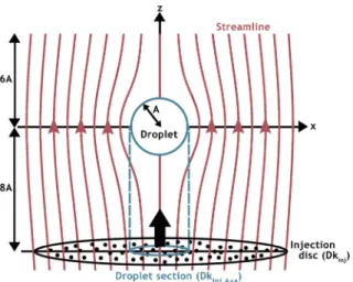
An injection disc of an AP, noted Dkinj, is set upstream of the droplet and centred on the Z axis as shown inFig. 1. The distance

between the disc and the droplet centre is far enough from the droplet to avoid any disturbance of the airflow by the droplet which could initially affect AP motions. It was found that 8 droplet radii A is a suitable distance, a wider distance increased the computation time without affecting the results. Downstream of the droplet, the APs are tracked up to 6A in case of rear captures due to the electrostatic forces, the Brownian motion or gravitational settling. The disc intercepted by the droplet in Dkinjis calledDkinj A a, + , equal

to a disc radius of the sum of the droplet (A) and AP (a) radii.

As inCherrier et al. (2017), the collection efficiency is evaluated by the ratio of the AP number set initially inDkinj A a, + over the AP

number collected by the droplet at the end of the computation (see section3.3.5). The AP coagulation is neglected in the model.

3.2. Flow field modelling

In the present model, droplets are set as simple collector since the in-cloud droplet concentration are overall low enough - about 50 droplets per cubic centimetre (Squires & Twomey, 1958) - to lead to a droplet-droplet mean distance larger than the mean boundary layer thickness. The assumption is made that the effect of the flow around the AP on the motion of the droplet can be neglected. Indeed, according toTinsley, Zhou, and Plemmons (2006), there is no significant disturbance on the airflow if the AP mass

mAP is more than thousand times lower than the droplet mass MA(m MAP/ A 103) as is the case in the AP and droplet ranges

considered here. Thus, the flow surrounding the droplet is only caused by its fall.

The internal circulation is not modelled in the current model since there is no effect on the external flow around the droplet. Indeed,LeClair, Hamielec, Pruppacher, and Hall (1972)have shown that for water droplet withRe<10the external flow patterns are insensitive to the interior flow and the drag coefficient for a rigid sphere differs by less than 1% from the drag coefficient for a fluid sphere. More recently,Oliver and Chung (1987)extended the computations ofLeClair et al. (1972)to moderate Reynolds number

(6)

<

Re 50. The maximum Reynolds number considered is the current paper is 7.42 ( =A 100µm).

The turbulence in the cloud can also have an impact on the AP collection and the collection efficiency since it may affect the APs/ droplets location and motion (Shaw, 2003). However, the effects of the turbulence have been neglected here.

A 3D computational domain must be used due to the Brownian motion which is a 3D process. Nevertheless, the airflow caused by the falling droplet is purely axisymmetric in the droplet range considered (A 100µm and Re 7.42, seePruppacher et al., (1998), Sect. 10.2). Thus, for every time step and every AP, we define the plane including the Z-axis and an AP (seeFig. 1) and we compute the airflow in this 2D computational domain in order to get the fluid velocity at the AP location Uf AP@ . The flow field modelling is subdivided into two cases following the droplet radius A.

3.2.1. A 30 µm - analytical expressions

For a low Reynolds number (Re 1), the non-linear term in the Navier-Stokes equation can be neglected. Thus, an analytical expression can be found which leads to the well-known Stokes flow expression. This solution results from the assumption that the advective inertial forces are small compared to the viscous forces - which is true near the droplet but incorrect for an increasing distance. This is called the “Stokes paradox”.

Here, the flow surrounding the droplet is modelled according toTinsley et al. (2006)- the Oseen (OS) expression is used far from the droplet ( >r* 5_{), the Proudman-Pearson (PP) expression near the droplet ( <}_r* ₂_{). A smooth transition is applied between both} expressions (2 r* 5_{) such as the weight is 0 (resp. 1) at =}_r* ₅_{for the OS expression (resp. PP) and 1 (resp. 0) at =}_r* ₂₍_r*_{, the} AP-droplet distance normalised by the AP-droplet radius A). Indeed, the OS expression corrects the Stokes paradox far from the AP-droplet. Thus, the PP expression is used near the droplet to solve this problem which is an asymptotic expansion between the Stokes flow and OS expression. The analytical expressions can be found inTinsley et al. (2006)where the terminal velocity of the droplet U ,Aand its

Reynolds number Re are both computed from the Beard model (Beard, 1976) - seeAppendix Afor more details.

3.2.2. A > 30 μm - numerical solver

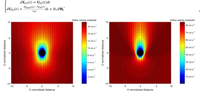
Beyond a droplet radius >A 30µm( >Re 0.41), a numerical solver (ANSYS CFX) is used in order to get more accurate airflow modelling. Two examples are illustrated inFig. 2for droplet radii 37.5 μm and 100 μm. The computational field of the simulation has been provided as[ 15,15]and [0,20] on the Z and X axis respectively and the square cell size was 2× 102_{(normalised by the droplet} radius). It is assumed the airflow is homogeneous beyond the computational field. Then, if an AP trajectory leaves the computational field in the X axis, the airflow velocity is set equal to the airflow velocity of the boundary at the same Z.

3.3. Analytical Lagrangian integration scheme used in the AP tracking

Since the major part of the AP radius range considered in the paper ([4 nm; 1.3 μm]) is smaller or comparable to the mean free path of air molecules (104 nm in an air temperature and pressure of 256.15 K and 540 hPa modelling the mid-troposphere) - the Brownian motion has to be considered. In the current paper, the Brownian motion modelling was performed following the Lagrangian approach ofLangevin (1908)where the vector force equations of a colloidal AP around a droplet are given byMinier and Peirano (2001)and used in several recent papers (Cherrier et al., 2017;Henry et al., 2014;Mohaupt, 2011;Mohaupt, Minier, & Tanière, 2011) summarised by: = = + d t t dt d t dt B d X U U W ( ) ( ) ( ) , AP AP AP Uf AP@ ( )t_APUAP( )t t ₍₃₎

Fig. 2. ANSYS CFX simulation - Airflow evaluating around a droplet of radius (a, left) 37.5 μm (U,A = 17.4 cm s−1, Re = 0.59) and (a, right)

100 μm (U,A = 82.4 cm s−1, Re = 7.43). The colors represents the airflow velocity amplitude while the arrows are the velocity vectors. (For

(7)

withXAPthe AP location vector, Uf AP@ the fluid velocity at the AP location,UAPthe AP velocity vector, t the time,B is the diffusion

coefficient accounting for Brownian motion and APthe AP relaxation time.dWtis the Wiener process increment which is a stochastic process modelling the random walk due to the Brownian motion of the APs.

These equations cannot be solved “classically” due to the Wiener process increment which is a stochastic process. In fact, tra-jectories are not bounded by a finite interval of time, pulling the stochastic integral out of the Riemann-Stieltjes rules. Hence, the stochastic integral calculation rules expressed byItô et al., (1965)are applied in Equation(3). The particle motion is finally obtained using the analytical Lagrangian integration scheme proposed byMinier and Peirano (2001)which is applicable regardless of the time step Δt (Equation(4)): + = + + + + + = + + +

(

)

(

)

(

)

(

)

t t t t e t t e B t B t t t e t e B e X X U U U U U ( ) ( ) ( ) 1 ( ) 1 2 ( ) ( ) ( ) 1 1 , AP AP AP AP f AP AP AP AP e e AP e e AP AP f AP @ 1 1 2 1 2 1 @ ₂ t AP APt t AP t AP t AP AP APt t AP APt AP APt 2 2 2 (4) where and represent independent vectors of random variables sampled in a standard normal distributionN(0,1), generated by

the Box-Muller method (Box & Muller, 1958).

This analytical Lagrangian integration scheme has been used in the recent paper ofCherrier et al. (2017)giving similar results compared to theWang et al. (1978)reference paper. The approach only considers the drag force and the Brownian motion, defined by the first and second terms respectively in the velocity variation in Equation(3). In the present paper, the buoyancy force Fbuoy(see

Appendix A) and the electrophoresis forceFelecare added. In order to use the analytical Lagrangian integration scheme proposed by

Minier and Peirano (2001)in Equation(4), a substitution is then applied and summarised in Equation(5):

= = + d t t dt d t dt B d X U U W ( ) ( ) ( ) , AP AP AP t t U U t ( ) ( ) f AP AP AP @ (5) where Uf AP@ is the resulting velocity at the AP location due to the added forces (Equation(6)):

= + + t t m Uf AP( ) Uf AP( ) AP(F F ) AP buoy elec @ @ (6) The analytical expression for the electrostatic forces is deduced from the image charge theory developed byJackson (1975)given by Equation(7): =

(

+

)

+

( )

Felec ₄q_A ₍_r r ₁₎ _r1 _r1·Q_q , 2 0 2 * *2 2 *3 *2 (7) where =r* r A/ _{is the normalised AP-droplet distance, A the droplet radius,}

0is the permittivity of free space, q and Q respectively the AP and droplet charge. In Equation(7), the first term dominates at short-range and is always attractive (due to the image charge of q inside the droplet with opposite sign). The second term, which is a Coulomb inverse square force, is repulsive or attractive depending on whether q and Q have unlike or like signs, prevails at long range with a weak amplitude compared to the image charge term. Further details can be found inTinsley, Rohrbaugh, Hei, and Beard (2000).

Each particle trajectory is then calculated by iteratively updating its position with the analytical Lagrangian integration scheme (Equation(4)) where Uf AP@ is substituted by Uf AP@ . It is assumed that there is no interaction between the APs during the compu-tation. Also, the droplet is considered unaffected by the electrostatic forces induced by the AP charge. As mentioned inGrover and Beard (1975), since the AP and the droplet acceleration are equal to the electric force divided by the respective masses, the ratio of the droplet acceleration over the AP acceleration is m MAP/ A 10 3(whereMAis the droplet mass) in the droplet and AP range

considered in this paper. Thus, the droplet acceleration is more than a thousand times lower than the AP acceleration which means the droplet motion is essentially unaffected during the AP travel around the droplet.

3.4. Boundary conditions 3.4.1. Injection disc

Initially, each AP is assigned an initial position according to a uniform statistical distribution. The initial velocity of each AP is set to the airflow velocity at the AP location. Far from the droplet, it is equal to (Equation(8)):

= = U U U (0) (0) 00 AP f AP A @ , (8)

(8)

optimised by following Equation(9):

= + + +

RDkinj A a xbro Axmax (9)

In this sum,A+ais the radius of a cylinder of air which contains all AP susceptible to be collected by the droplet during its fall (impaction and interception processes).xbroextends this cylinder to account for the maximum AP displacement possible due to the

Brownian motion. The Fokker-Planck equation is used to evaluatexbro(Equation(10)):

= P x x t D t x x D t ( | , ) 1 4 exp ( ) 4 , b b 0 1 1 1 02 1 (10)

where Dbis the Einstein-Stokes coefficient,x0the initial AP location and t1the AP time spent betweenx0and x. P x x t( | , )0 1 is the likelihood of being at the AP location x given the initialx0location after t1. To evaluatexbro, t1is set to the distance of the injection disc from the droplet over the droplet terminal velocity ( =t1 8 /A U ,A). Moreover,xbrois computed for every AP radius by considering a

likelihood of 99.9%, settingx0 to zero. This means, 99.9% of the AP assigned in the injection disc will statistically have a dis-placement due to the Brownian motion belowxbro.

To account for the electrostatic forces, a 2D Lagrangian tracking is used in order to get the initial maximum distancexmaxfrom the

axis Z (normalised by the droplet radius) which lead to the AP collection. The AP is injected upstream from the droplet at a distance of 8A where it is assumed the airflow is not affected by the droplet. The drag force and the electric effects are only considered in this calculation (no weight, no inertia and no Brownian motion). The integration scheme is the same as the one described inTinsley et al. (2001). However, the airflow is still computed according to section3.2.

3.4.2. AP number in the injection disc

The APs are injected following a uniform statistical distribution. One thousand APs are initially injected in the disc intercepted by the droplet (Dkinj A a, + ). Then, the whole injection discRDkinjis randomly filled with the same density thanDkinj A a, + . A first realisation

(initialisation of the injection disc and computation of the AP trajectories) is provided in order to get a first evaluation of the number of APs collected by the droplet NAP col, . IfNAP col, <1000APs collected, the initialisation of the injection disc is restarted and extra AP are injected until 1000 AP collections to ensure a reliable number of significant figures and to converge quickly following the Monte Carlo method (see section3.4.5).

3.4.3. AP capture conditions

It is assumed that the APs stick to the droplet once they collide with it. The retention efficiency is set to unity. Thus, an AP collection occurs as soon as an AP touches the droplet surface and its tracking is over. In addition, if an AP leaves the computational domain without collision with the droplet, the collection is missed and the modelling of its movement finishes.

The first type of AP collection happens at the end of a time step when the AP distance from the droplet is lower than the sum of the AP and droplet radius. The first condition is given by Equation(11). Whereas this condition includes all types of scavenging effects (Brownian, phoretic and dynamic), a second condition refers to only the Brownian capture occurring during large time steps. This second condition is based on the bridge theory (Henry et al., 2014) summarised by Equation(12). Moreover, when the AP distance from the droplet is very low, the AP pass sometimes through the droplet during a time step due to the electrostatic force tends to infinity whenr* _{tending to unity (Equation}₍₇₎_{). Instead of decreasing the time step to face this strong force close to the droplet} (increasing the calculation time), a third AP collection is considered in the model. As a result, if the APs cross the droplet during a time step, it is considered as collected.

= + = d_{AP d} (X X ) (A a) i AP i d i , 2 1 3 , , 2 2 (11) where XAP i,(resp. Xd i,) is the position of the AP (resp. the droplet centre) on the axis i, n the dimension of the computational domain

and dAP d, is the droplet-AP distance.

= + = + + = = + + + + d t X t X t d t t X t t X t t ( ) ( ( ) ( )) ( ) ( ( ) ( )) , AP d i AP i d i AP d _i AP i d i exp 1 exp 1 , 1 3 , , 2 , 3 ₁ , , 2 A a dAP d t dAP d t t A a B AP t dAP d t dAP d t t B _{AP t} 2( )( , ( ) _{2 2}, ( ) ) 2 , ( ) , ( ) 2 2 (12) where λ is a random variable sampled in a uniform distribution.

3.4.4. Time step

The analytical integration scheme (Equation(4)) ofMinier and Peirano (2001)can handle the both borderline cases of the ballistic ( t AP, AP motion mosly governed by the dynamical effects) and diffusion ( t AP, AP motion mostly governed by the

Brownian motion) regimes. Then, Δt varies from103× APto10 1× APwhen a varying from 4 nm to 1.3 μm with a factor 1, 1/2, 1/3,

(9)

3.4.5. AP collection efficiency determination

The collection efficiency is defined as the ratio of the number of AP collected NAP col, by the droplet over the number of AP initially included inDkinj A a, + assigned asNAP Dk, inj A a, + (Fig. 1). This parameter depends on the droplet radius A, the AP radius a, the relative

humidityRH due to the thermo- and diffusiophoresis forces, the AP and droplet charge (q and Q) caused by electrostatic force (Equation(13)): = + Ec i,( , , , ,a A q Q RH) _N NAP col( , , , ,a A q Q RH_{( , , , ,}_{a A q Q RH})i ₎ AP Dkinj A a i , , , (13)

Thus, the collection efficiency is determined by initialisation of the injection disc (see section3.4.1). Every AP trajectories are computed related to the analytical Lagrangian scheme described in Equation(4)and the NAP col, is updated online following the three AP capture conditions described in section3.4.3. The AP collection by the droplet is a stochastic process through the Brownian motion integrated into the AP vector forces (Equation(5)). The capture efficiency Ecis then computed using a Monte Carlo method

according toCherrier et al. (2017). Indeed, Ecis obtained by averaging a set of n successive realisations (Equation(14)) where a

realisation involves the initialisation of the APs in the injection disc, the computation of all trajectories until the APs are collected or missed by the droplet (i.e. the APs leave the computational domain downstream of the droplet). In the present model, 50 realisations are computed in order to get a reliable value of the collection efficiency (see section3.5).

= ₌ E a A q Q RHc( , , , , ) _n i E ( , , , ,a A q Q RH), n c i 1 1 , (14)

where Ec i,is the collection efficiency computed at the i-th realisations.

3.5. Validation and convergence

AsCherrier et al. (2017), the Browian motion modelling has been verified. The root mean square displacement of the particle is compared to the theoretical expression x t()2 _of_{Einstein (1956)}_{given in Equation}₍₁₅₎_.

=

x t2( ) 2D D tim b , (15)

whereDimis the dimension of the computational domain and t the computational time.

The flow velocity at the AP location disturbed by the added forces U*f AP@ is set to zero in the analytical integration scheme (Equation(4)). The initial AP velocity is zero and the AP location is the origin of the Cartesian coordinate system. The number of time step for each AP is computed to have an integration time of 10 ms. To compare the Brownian motion in the simulation to theory, the root mean square displacement is calculated from 4000 AP trajectories for each AP radius. It results a discrepancy less than 1% is observed between the model and the theory for the whole AP radius range.

Furthermore, we have verified the airflow velocity convergence. The meshes are generated through ANSYS CFX where the grid used for the discretisation is unstructured and composed of quadrilateral cells whose mesh density increases near the drop surface. Then, the meshes are post-processed in order to get a uniform grid from the raw data. A cell size is set to ensure that the results are independent of the resolution. Indeed, it was verified that the collection efficiency did not vary if the grid is refined. It was found that a cell size of 2× 10 2_{(normalised by the droplet radius A) is suitable. During a realisation, the exact values are computed through} interpolations.

The injection disc radius (RDkinj) convergence has been verified in a third validation test in order to ensure the collection efficiency

is unaffected by the increasing of theRDkinj.

Fourth, the statistical convergence of the collection efficiency Ec has been ensured. In the current model, the number of AP

injected is set to have at least 1000 APs collected by the droplet during every realisation. A Shapiro-Wilk test (Shapiro & Wilk, 1965) with a significance level of 95% is computed to verify that the obtained efficiencies are normally distributed. After which, the confidence interval on Ecis estimated through a Student-t distribution test with a level of 95%. For at least 1000 APs collected, it was

found that 50 realisations allow computing Ecwith a confidence interval of 2% for a 4 nm AP radius (sensitive to Brownian motion)

whereas a 1.3 μm AP radius (non-sensitive to Brownian motion) gives a confidence interval smaller than 0.01%.

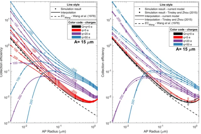
Finally, the present Lagrangian model has been tested under mid-tropospheric conditions (Tair= 256.15K, Pair=540 hPa,

RH = 100%) with an AP density of 500 kg m-3_{presented in}_{Fig. 3}_{a. Thus, the current model has been compared to the}_{Tinsley and}

Zhou (2015)model (Fig. 3b). The results are very close to theTinsley and Zhou (2015)values, which confirms the performances of the model. Note that it is not a direct comparison sinceTinsley and Zhou (2015)consider the collision rate coefficientRc(also called

collection kernel) instead of the collection efficiency Echere. In order to compare both data model, theTinsley and Zhou (2015)data

have been formulated in Ecsince both quantities are directly correlated (seeAppendix A).

It is important to emphasize that the variations are really different considering Ecinstead ofRc. Indeed, while the Ecin general

decreases with increasing droplet radius (Fig. 4),Rcincreases since the terminal velocity of the droplet and the cross sectional area

both increase rapidly (their product increases approximately as the fourth power of droplet radius up to about 50 μm radius). 4. Results of simulation and discussion

All numerical results are given as table in supplementary material. Simulations have been performed to evaluate the collection efficiency for 13 AP radii0.004 a 1.3 µmand 6 droplet radii A = 15, 25, 37.5, 50, 75 and 100 μm - following the conditions

(10)

summarised inTable 2. The AP charge q is set to 0, 5, 20, 50 and 600 e, in order to model the AP charge which can appear in clouds for a non-radioactive and radioactive AP case (section2.2). The droplet charge is set - from the electrically neutral case to the electric charge Q according toTakahashi (1973)for both stratiform and convective cloud case - depending on the droplet radius referred to Table 1. A relative humidity of 100% is considered to ensure no diffusiophoresis and thermophoresis effects on the collection efficiency. The simulations have been made for mid-tropospheric conditions ( 17oC_{, 540 hPa) and an average AP density of}

kg m

1500 . 3_{. It should be noticed that the collection efficiencies below 10}−5_{have been determined but not been statistically}

con-verged to reduce the computation time. Results below 10−5_{are then not presented here.}

4.1. Case without electrostatic forces ( = =q Q 0e)

Fig. 4shows the collection efficiency (EC) related to the AP radius for the whole droplet size range considered in the study. The points represent the numerical results of the current model and the dashed lines refer to the collection efficiency ECWangrelated to the

diffusion kernel KWangofWang et al. (1978)whereECWang KWang/( ·U ,A· (A+a) )2 (expressions can be found inAppendix A).

The following results can be noticed:

•

No matter the droplet size, for an AP radius smaller than 40 nm, a decrease of the EC is observed when the AP radius increases. More precisely, it can be noticed that our simulations perfectly fit ECWangwhich means that the EC is purely driven by the

Brownian motion for these AP sizes. This is the reason why, for a given AP size, the EC decreases for larger droplet radii. Also, for an increasing droplet radius, the travel time of the AP around the droplet decreases with a higher airflow velocity. Thus, the AP collection due to the Brownian motion has less time to operate (since x t2( ) _{is proportionate to t in Equation}₍₁₅₎_{). It is}

worthwhile to note that the collision rate efficiency has the opposite variation here - increasing for smaller droplet radii (Zhang, Tinsley, & Zhou, 2018). This is due to the ventilationfpin the diffusion kernel KWang(Appendix A) ofWang et al. (1978)which

increases with the shorter interaction times. In fact, there is less depletion of the AP concentration by the immediately preceding scavenging in the air that the droplet is falling through.

•

For small droplets (A 37.5µm)

– For 40 nm a 0.5µm, the collection efficiency keeps decreasing for larger particles but there is a difference between the

Fig. 3. (a, left) Collection efficiency for the whole AP radius range and few cases of AP and droplet charges under the mid-tropospheric conditions

(Tair=256.15K,Pair=540hPa, RH = 100%) and an AP density of 500 kg m-3. The red, purple and blue curves represent an AP charge of 5, 20 and

50 e respectively. The droplet charges are directly mentioned on the curves (in e). Dotted lines are the extrapolation when an EC value is below 10−5_{. The points are the simulation results meanwhile the dashed lines are the collection efficiency EC}

Wangcoming from the well-known diffusion

kernel ofWang et al. (1978). (b, right) Indirect comparison between the current model (solid line) and theTinsley and Zhou (2015)model (dotted line).

(11)

current model - which gives higher values - and the model ECWangofWang et al. (1978). Indeed, the larger the AP radius is, the

more significant the discrepancy is. In this AP size range, the collision between the AP and the droplet is still dominated by the Brownian motion, nevertheless, inertia mechanisms cannot be neglected any more. On the one hand, the effect of the Brownian motion declines and the mean AP displacement relatively to the streamlines decreases, and on the other hand, the intercept effect increases - which intensifies for large AP and small droplets. It should be noted that the AP inertia also plays a small but increasing role in the AP radius range for wider AP and droplet radii. So, for A 37.5µmand 40 nm a 0.5µm, the efficiency is still dominated by the Brownian motion but the relative contributions of the interception and the inertia increases. – To explain the large decrease of the collection efficiency for0.5µm<a 1.3µmand A 37.5µm, a simple case without diffusion is considered. The trajectory of an AP injected on the droplet axis - the coordinate system is centred on the falling droplet - is computed and the AP goes up and slows down near the droplet because of the airflow velocity which falls to zero at the droplet interface. For those droplet radii, there is a stagnation region (Zhang & Tinsley, 2018) beyond the collection limit -sum ofa+A- where the AP falls faster than the upward airflow. Then, since there is not enough inertia and the diffusion and phoretic forces are neglected, the AP comes to rest relatively to the droplet and will never be collected. Also, if the AP is injected

Fig. 4. Results of the simulations for the whole droplet radius range under the mid-tropospheric conditions (Tair=256.15K,Pair=540 hPa,

RH = 100%) without electric charges on the droplet and AP ( = =q Q 0e). The solid lines are the fittings of the simulation results and the dashed lines are ECWang- the collection efficiency related to the diffusion kernel ofWang et al. (1978).

Table 2

Conditions of simulation.

Parameter Numerical value

Air density - air 0.73 kg m−3

Air pressure - Pair 540 hPa

Air temperature - Tair 256.15 K

Air viscosity - air 1.63× 10 5kg m−1.s−1

AP density - AP 1500 kg m−3

AP radius - a ∈[4 nm; 1.3 µm]

Droplet radius - A 15/25/37.5/50/75/100 μm Mean free path of air molecules - air 104 nm

Relative humidity - RH 100%

Reynolds number - Re 0.04/0.18/0.59/1.30/3.70/7.43 Terminal velocity of the droplet - U ,A 3.01/8.16/17.4/28.8/54.8/82.4 cm s−1

(12)

nearby the ascending axis, the AP approaches the droplet until it reaches this stagnation region. At this point, the AP does not move following the ascending axis but horizontally moves to the side due to the horizontal component of the airflow velocity. These both cases are illustrated inFig. 1ofZhang and Tinsley (2018). Therefore, the collection efficiency drops while the AP weight increases with its radius. This effect is strongly dependent on the AP density (Zhang & Tinsley, 2018).

∗Accordingly, for =A 15µm, the collection efficiency does not collapse to zero thanks to the Brownian motion which allows either for the AP to be collected in the stagnation region or to come closer to the collection limit for AP initially from the side. For =A 25µm, the reduction of the collection efficiency is greater than for =A 15µmsince it is less likely for the AP to come closer to the collection cross section through the effect of the Brownian motion. It should be noticed that, in both cases, the AP inertia can also improve the AP collection in the stagnation region but this mechanism has second-order importance com-pared to the Brownian motion.

∗In the case of =A 37.5µm, the collection efficiency still decreases but not as much as for =A 25µmfor two reasons. First, the AP inertia is not a second-order process any more in the AP collection. Also, the stagnation region beyond the distance of collection is reduced because the airflow velocity is faster for larger droplets and the normalised collection limit is smaller.

•

There is a minimum collection efficiency computed by the model which can be seen for =A 75µmand =A 100µm, but occurs at

>

a 1.3µmfor the smaller droplets (not shown). It can be observed that, for an increase of the droplet radius, this minimum of what is called “Greenfield gap” (Greenfield, 1957) - moves to smaller APs. Also, the collection efficiency starts to become higher than ECWangfor a smaller AP when a larger droplet is considered. These variations come from the AP inertia which becomes more

and more important when the mass is increasing as the cube of the AP radius. Indeed, the inertia becomes so strong that the AP continues upward relative to the droplet and impacts it.

4.2. Case with varying droplet and AP charges

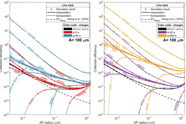
Simulation results are presented inFigs. 5–10, corresponding respectively to droplet radii from 15 to 100 μm. The collection efficiencies related to the diffusion kernel ofWang et al. (1978)are also referred to as a dashed line for every droplet radius (ECWang).

In all the figures, the points indicate the simulation results, the red, purple, blue and yellow curves represent an AP charge of 5, 20, 50 and 600 e, respectively. The droplet charges are directly mentioned on the curves in number of elementary charge (e) (seeFig. 7).

Fig. 5. Results of the 15 μm droplet radius under the mid-tropospheric conditions (Tair=256.15K,Pair=540hPa, RH = 100%). The points are the

simulation results meanwhile the dashed lines are the collection efficiency ECWangrelated to the diffusion kernel ofWang et al. (1978). The red,

purple, blue and yellow curves represent an AP charge of 5, 20, 50 and 600 e respectively. The droplet charges are directly mentioned on the curves (in e). Dotted lines are the extrapolation when an EC value is below 10−5_{. (For interpretation of the references to color in this figure legend, the}

(13)

First, the trends without electrostatic forces observed in the previous section, are still visible for large AP even though strong AP and droplet charges are key in reducing their effects. The contributions of both terms in the electrostatic forces’ expression (Equation (7)) can be observed in the simulation.

4.2.1. Domination of the short-range attractive term

For zero droplet charge, the contribution of the Coulomb inverse square term in Equation (7)is zero (curves labelled 0 in Figs. 5–10). In this case, it can be observed that the EC increases with the AP charge q, this agrees with results fromTinsley et al. (2000)andJaworek et al. (2002). This is due to the short-range attractive force between the AP charge and its image inside the droplet which is proportional toq2_{. Also, for zero droplet charge and a given AP charge q and droplet radius A, the factor by which the} collection efficiency increases compared to the curve without electrostatic forces ( = =Q q 0e) is reduced when the AP radius a is decreased. The relative magnitude of the contribution of the short-range attractive term declines for small AP radius since the Brownian motion becomes the major part of the AP collection, even if the absolute effect of the electrostatic term increases since the electric mobility of the AP is higher. Also, the short-range attractive term dominates near the Greenfield gap - in which the effect of the Brownian motion becomes weak and the dynamical effects (inertia and interception) are not yet large enough - and the dom-ination extends towards the small AP radius when the AP charge is increased.

Note that this is valid for the droplet charge Q near zero. On the contrary, the contribution of the short-range image charge attractive term is second-order compared to the Coulomb inverse square term for strongly electrified droplets.

4.2.2. Domination of the coulomb inverse square term

For the strongly electrified droplet computed in the present paper, the effect of the droplet charge Q exists for the whole AP size range considered in this paper. Indeed, for large product ×q Q, the Coulomb inverse square force dominates at large distance over the dynamical effect, even though the electric mobility of the AP is small. Thus, for large AP, the collection efficiency is increased or decreased depending on whether the Q and q have unlike or like signs and also the product ×q Q. For a small AP charge ( =q 5e) typical of the atmospheric AP with a droplet charge naturally found in a convective cloud ( =Q 10000efor =A 15µmor =Q 30000e

for =A 25µm), simulations have shown that the Coulomb inverse square term is so repulsive that the whole collection efficiencies in the AP size range studied are bellow10 5_.

(14)

For the weakly electrified droplet (Q ±102e_for _A₌₁₅_µm_,_Q _±₁₀3_e _for _A₌₁₀₀_µm_{), the contribution of the Coulomb} inverse square force increases for decreasing AP radius a. It can be observed through the effect of the droplet charge Q which is minor for AP larger than about 0.3 μm and become more and more important for tiny AP radius a no matter the droplet charge polarity - in line with the simulation ofTinsley and Zhou (2015). This is mainly due to the AP electric mobility which is proportional to the inverse AP radius a.

The domination of the Coulomb inverse square term can also be illustrated with:

•

The decrease of the EC when the Coulomb inverse square force is repulsive appears for small AP.

•

The curves with the products of the AP and droplet charges ×q Qequal and negative tends to the same value of EC for small AP. For example, inFig. 8the curve for =q 5eand =Q 10000ecoincides with the curve for =q 50eand =Q 1000eas the AP radius a is reduced. This is due to the Coulomb inverse square force which dominates at large distance for small AP and which is proportional to ×q Q far away from the droplet.

4.2.3. The transition region between both dominations

For same sign AP and droplet charges, the transition from the domination of the Coulomb inverse square force to the one of the short-range attractive force is evident in the simulation results. The larger the droplet and AP charges are, the more the transition appears for large AP radius a. For example, forA=15µm(Fig. 5), for =q 600eand =Q 100e, the EC is led by the short-range attractive force for AP larger than30nmsince the values are bigger than the case without electrostatic effects ( =q 0eand =Q 0e). For <a 30nm, the EC collapses and tends to zero when the AP radius decreases. Indeed, the Coulomb inverse square force opposes to the dynamical effects and prevents the AP from getting closer to the droplet and from involving the contribution of the short-range attractive force in the AP collection. The EC keeps decreasing for small AP because the repulsive force keeps getting stronger through an increasing AP electric mobility.

4.2.4. Impact of the droplet radius on the electrophoresis

The EC is less influenced by the electrostatic effects for a given AP radius a and an increasing droplet radius A. It can be observed for both terms in Equation(7):

Fig. 7. Results of the 37.5 μm droplet radius under the mid-tropospheric conditions (Tair=256.15K,Pair=540hPa, RH = 100%). The points are the

(15)

•

For example when =a 1.3µmand =Q 0e, the EC is enhanced by more than two orders of magnitude when the AP charge q varies from 0 to 600 e considering a droplet sizeA=15µm (Fig. 5), and by less than one order of magnitude for a droplet radius

=

A 100µm(Fig. 10).

•

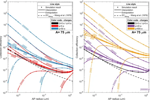
For =a 4nmand =q 20e, the effect of the droplet charge =Q 200eand200ecompared to the case =Q 0erespectively leads to a EC discrepancy from +595% and −99.9% for a droplet radius =A 15µm(Fig. 5), to +23% and −23% for a droplet radius

=

A 75µm(Fig. 9).

It can be explained through an increase of the airflow velocity which enhances the dynamical effects. Then, the AP inertia becomes important in reducing the contribution of the electrostatic forces but also any kind of phoretic forces as developed in the work ofWang et al. (1978). That is why in our study we consider strongly electrified clouds from theTakahashi (1973)measurement since the weak droplet charges Q used inTinsley and Zhou (2015)have a minimal effect on the EC for large droplets. Indeed, for

=

A 100µm, the highest difference (for the minimum AP radius =a 4nm) between the case =Q 300eand =Q 0eis less than +6% when the AP is weakly electrified ( =q 5e) and almost +37% in the extreme case where the AP is radioactive ( =q 600e). Never-theless, a weak AP charge characterising the atmospheric AP must be studied since its effects on the EC is strong - coupled with a droplet charges Q which can be found in clouds. For =A 100µm, =a 4nmand =q 5e, the EC increases by a factor of 176 if a droplet charge =Q 400000erather than the neutral case ( =Q 0e) is considered.

5. Conclusion

Simulations were performed for a similar range of AP radius studied inTinsley and Zhou (2015)through a novel theoretical model of collection efficiency computation which models the Brownian motion with the Langevin approach (1908). A wide range of AP and droplet charges have been considered as typical for the atmospheric AP but also for a radioactive AP released after a nuclear accident like Fukushima. The present paper extends the simulation ofTinsley and Zhou (2015)by computing a wide range of droplet radii from15µmto100µmand widens the droplet charge interval to strongly electrified clouds in order to study the electrostatic forces which can appear in stratiform and convective clouds through the Takahashi measurements (1973). It results a large contribution of the electrostatic forces in the collection efficiency (EC) for the wide range of droplet radii. Indeed, the EC is increased up to 4 orders

(16)

of magnitude with a droplet and an AP charge representative of convective clouds and radioactive AP, respectively. An EC en-hancement has also been found for AP (q) and droplet (Q) charge of same signs for cases where the product ×q Qis moderate, however the EC collapses below 10−5_{for large products of charge.}

Simulations must be applied with caution when an AP density other than that computed in the paper is considered. For large AP, the effect of the AP inertia enhances the EC for increasing AP density. Also, for small droplet radii (A 37.5µm), the contribution of the AP weight is highly dependent on the AP density as shown byZhang and Tinsley (2018)orZhang et al. (2018,Fig. 6). Thus, most of the simulations have to be repeated when the AP density strongly differs from 1500 kg m−3_{. Nevertheless, for zero charge on the}

droplet ( =Q 0e), the effect of the AP density is not significant for small AP radius even though there is non-zero charge on the AP (q 0e). For example, the discrepancy of the EC when the AP density differs from 500 to 4500 kg m−3_{is less than 4% and 2% for}

=

q 0eand =q 50erespectively, for an AP radius smaller than 80 nm.

To apply the simulation results outside mid-tropospheric conditions (-17°C, 540 hPa),Fig. 8fromTinsley and Leddon (2013)can be used to estimate the effect of altitude on the collection efficiency. Taking high-tropospheric conditions at altitude 12.5 km (-56°C, 180 hPa) or tropospheric conditions at the surface of the Earth (+15°C, 1013 hPa), the discrepancy is less than 40 and 20% re-spectively. Finally, to extend the present simulations for other droplets radii, droplet and AP charges, interpolation or moderate extrapolation can be made. The model is also suitable to investigate the impact of the thermophoresis and the diffusiophoresis on the collection efficiency - which have not been studied in the current paper - by getting the temperature and vapour density fields around the droplets and by adding the analytical expression of the forces in Equation(6).

These simulations can also be used for a wide range of applications like climate models, pollution models or cloud models with detailed microphysics like DESCAM (Flossmann, 1998). It is necessary to first obtain the charge distributions on the AP and the droplets. Also, for real situations, the collection efficiencies must be integrated over charge and size distributions of APs and droplets. It provides a simple base for modelling the changes in AP concentration, the ice-forming nuclei in clouds which in turn can impact precipitation or the Earth's energy budget. We plan to predict the radionuclide transfer in the environment after an accidental discharge into the atmosphere and those results are essential for the investigation. An important issue remains the experimental validation of the current model which has not yet been performed.

purple, blue and yellow curves represent an AP charge of 5, 20, 50 and 600 e respectively. The droplet charges are directly mentioned on the curves (in e). Dotted lines are the extrapolation when an EC value is below 10-5_{. (For interpretation of the references to color in this figure legend, the}

(17)

Appendix A. Nomenclature

Parameter Meaning Expression or Value Unit Source

a AP radius – m – AP Aerosol particle – – – A Droplet radius – m – BAP Particle mobility Cu air a 6 Kg -1_.s _{Tinsley et al. (2001)}

BBeard Beard (1976)constant ×

+ × × × × + × × + + 0.318657 10 0.992696 10 0.153193 10 0.987059 10 0.578878 10 0.855176 10 0.327815 10 1 0 2 3 3 4 5 – Beard (1976)

B Diffusion coefficient accounting for Brownian motion kbTair mAP AP

2 _{m. s} 3

2 Minier and Peirano

(2001) c Distance of the point charge q from A

r

2 _m _{Jackson (1975)}

the droplet centre

Cu Stokes-Cunningham slip correction factor

+ + e K

1 1.257 0.4 Kn n

1.10 _– _{Pruppacher et al., 1998}_),

Sect. 11.2

dAP d, Droplet-AP distance – m –

Db Einstein-Stokes coefficient CukbTair

air a

6 m

2_.s1 _{Pruppacher et al., (1998)}_,

Sect. 11.2

Dim Computional domain dimension 3 – –

Dkinj Injection disc of AP – – –

(18)

+

Dkinj A a, Cross-sectional area intercepted by the droplet in Dkinj (A+a)2 _m2 _–

dWt Increment of the Wiener process – _s1₂ Minier and Peirano

(2001)

Ec Collection efficiency – – –

Emax Maximum beta particle energy for the Caesium-137 decay 5.12× 105 eV –

ECWang Collection efficiency of Wang et al. (1978)

+ KWang U A A a, ( )2

– Wang et al. (1978)

f_A Droplet size distribution – m-3_.m-1 _–

Fbuoy Buoyancy force – N Grover and Beard (1975)

Felec Electrophoresis force – N Tinsley et al. (2006)

fp Particle ventilation factor ₁₊_{0.530 exp}_N _N1.1 – Tinsley and Zhou (2015)

f t( ) Random function – – –

g Acceleration of gravity 9.81 m.s-2 _–

gnet Net acceleration of gravity AP airg

AP m.s

-2 _{Grover and Beard (1975)} I Number of ion pair production per decay Emax

i

3 – Clement and Harrison₍₁₉₉₂₎

kb Boltzmann constant 1.38× 1023 m2.kg.s

-2_.K-1 –

Kn Knudsen number air

a – Pruppacher et al., (1998)_{Sect. 11.1} ,

KWang Diffusion kernel of Wang et al. (1978) 4 Af Dp b m3.s1 Wang et al. (1978)

MA Droplet mass – kg –

mAP AP mass 4 a _AP

3 3 kg –

N Cube root of the Péclet number _{AU A}

Db

2 , 13 – Tinsley and Zhou (2015)

n Concentration of the negative ions – m-3 _{Clement and Harrison}

(1992)

nb Background negative ion concentration 109 _m-3 _{Clement and Harrison}

(1992) NAP col, Number of AP collected by the droplet – – –

+

N_{AP Dkinj A a}, , Number of AP initially inDkinj A a, + – – –

Pair Air pressure – Pa –

P x x t( | , )0 1 Likelihood of being at the AP location x given the inital x0location

after t1

– – –

q AP charge – C –

q Image of the AP charge q A_rq C Jackson (1975)

q" Residual charge Q q C Jackson (1975)

Q Droplet charge – C –

q_mean Mean radioactive AP charge – C –

r AP distance from the droplet centre – m –

R Cartesian coordinate system (X, Y, Z) – –

Rc Collision rate coefficient Ec (A+a U) |2 ,A U ,a| m3.s-1 – +

Ec (A a U)2 ,A – –

RDkinj Radius of the injection disc A+a+x t( )+Axmax m –

Re Reynolds number

₍

₁₊_2.51air

₎

_exp

A YBeard

2 – Beard (1976)

r* _{Normalised AP distance from} r

A – –

the droplet centre

RH _{Relative humidity of air} _– _– _–

t Computational time – s –

t1 Time spent to the AP to go from A

U A

8

, s –

the injection disc to the droplet

Tair Air temperature – K –

UAP AP velocity vector – m.s-1 –

Uf AP@ Fluid velocity at the AP location – m.s-1 –

ur Unit vector in the radial direction – – –

u Unit vector in the orthoradial direction – – –

U_{f AP}_@ Resulting velocity at the AP location – m.s-1 _–

due to the added forces

U,A Terminal velocity of the droplet air Re A air

2 m.s

-1 _{Beard (1976)} U,a AP fall speed disturbed by the added forces – m.s-1 –

Wt Wiener process – _s1₂ Minier and Peirano

(2001)

XAP AP location vector – m –

XAP i, AP position on the axis i –

XBeard Beard (1976)constant

log A g air w air air

32 3 ( ) 3 2