HAL Id: hal-00908770
https://hal.archives-ouvertes.fr/hal-00908770
Submitted on 25 Nov 2013
HAL is a multi-disciplinary open access archive for the deposit and dissemination of sci-entific research documents, whether they are pub-lished or not. The documents may come from teaching and research institutions in France or abroad, or from public or private research centers.
L’archive ouverte pluridisciplinaire HAL, est destinée au dépôt et à la diffusion de documents scientifiques de niveau recherche, publiés ou non, émanant des établissements d’enseignement et de recherche français ou étrangers, des laboratoires publics ou privés.
To cite this version:
C. Corbane, S. Alleaume, M. Deshayes. Mapping natural habitats using remote sensing and Sparse partial least square discriminant analysis. International Journal of Remote Sensing, Taylor & Francis, 2013, 34 (21), p. 7625 - p. 7647. �10.1080/01431161.2013.822603�. �hal-00908770�
1
Mapping natural habitats using remote sensing and Sparse Partial Least
Square Discriminant Analysis
C.CORBANE, S. ALLEAUME and M.DESHAYES
Irstea – UMR TETIS, Montpellier, France
Campus international de Baillarguet TA C-91 / F (Bldg. F, Off. 207 b- 34398 Montpellier Cedex 5), France; e-mail: [email protected]
2
Mapping natural habitatsusing remote sensing and Sparse Partial Least
Square Discriminant Analysis
This work presents a novel approach for mapping the spatial distribution of natural habitats in the “Foothills of Larzac” Natura 2000 listed site located in a French Medi-terranean Biogeographical Region. Sparse Partial Least Square Discriminant Analysis was used to analyze two RapidEye datasets (June 2009 and July 2010) with the purpose of choosing the most informative spectral, textural and thematic variables that allow discriminating the classes of habitats.The Sparse Partial Least Square Discriminant Analysis selected relevant and stable variables for the discrimination of habitat classes that could be linked to ecological or biophysical characteristics. It also gave insight into the similarities and the differences between habitats classes with comparable physiog-nomic characteristics. The highest user accuracy was obtained for dry improved grass-lands (u=91.97%) followed by riparian ash woods (u= 88.38%). These results are very encouraging given that these two classes were identified in Annex 1 of the EC Habitats Directive as of community interest.Due to limited data input requirements and to its computational efficiency, the approach developed in this paper is a good alternative to other types of variable selection approaches in a supervised classification framework and can be easily transferred to other Natura 2000 sites.
Keywords: Dimension reduction; RapidEye, Natura 2000, Dry improved grasslands, Riparian ash woods.
1. Introduction
Loss,fragmentation and degradationof natural habitatsoccurworldwideand areprimarily due to thepressures ofincreasinghuman population, rapid urbanization andunsustainable useof natu-ral sites. Within the European Union (EU), only 17% of species and habitats and 11% of EU-protected ecosystems are doing well. The rest are under pressure, mainly from human activi-ties, or are in decline (European Commission, 2011). To face the current and future threats to biodiversity and habitats loss, several initiatives at different levels have been launched in the last decades. In the European Union, the Habitats Directive adopted in 1992, imposes on EU member states the conservation of rare and/or threatened habitats and species of ‘Community
3 interest’ (i.e. those habitats and species listed in annexes to the Directive). Articles 11 and 17 of the Directive also require member states to report on four parameters of habitat conserva-tion status every six years: habitat area, range, indicators of habitat quality, and future pros-pects for habitat survival in the member state (European Commission DG Environment 2007; Vanden Borre et al. 2011).Article 3 sets up a “coherent European ecological network of spe-cial areas of conservation”, called the Natura 2000 network.Today this network covers more than 25,000 sites and makes up around 17% of the total area of the EU. It is the largest net-work of protected areas in the world and the backbone of the Pan-European Ecological Net-work. One of the main challenges for the implementation of Natura 2000 network is the de-sign of accurate and simple methods for a continuous and consistent monitoring on the state and spatial extent of sensitive habitats (Bock 2003; Bocket al. 2005; Díaz Varela et al. 2008). Owing to their exhaustive and systematic coverage of the territory, the frequent repeated measurements and the possibility of obtaining quantitative data at high sampling densities, remote sensing techniques have been long regarded as an attractive option for cost effective generation of environmental data and for natural habitats mapping, particularly in Natura 2000 areas (Weiers et al. 2004).
Remote sensing can contribute to a better understanding of the diversity of natural and semi-natural habitats, their spatial distribution and their conservation status. This has been established by several studies and reported in many review papers like those of Nagen-dra(2001), Turner et al. (2003), Kerr and Ostrovsky(2003) and more recently Nagendra et al. (2012). Despite the large number of studies cited in these reviews, there is evidence that the vast majority of remote sensing works focuses on the delineation of land cover categories rather than on detailed mapping of habitat types which reveals to be much harder to under-take.
4 Few studies addressed the topic of classification of remote sensing data into detailed and complex habitat types. Bock (2003) attempted to use Landsat imagery to define spectral-ly homogeneous vegetation types (e.g. meadows, woody brushes, coniferous and grassland) and then to establish a content-wise correspondence of these classes with the biotope and use types. The major limitation of the developed approach was in the recognition of woody scrubs on water-logged soils that were partly under- or overestimated. In Keramitsoglou et al. (2005), very high resolution satellite imagery acquired over different Natura 2000 sites (lo-cated within different biogeographical regions (BGR)), was analyzed with a kernel-based classification algorithm for mapping fine scale habitats according to the EUNIS (European Commission DG Environment 2007) classification schema. This allowed a consistent com-parison of the performance of the algorithm across the different sites. The results on the site located in the Atlantic BGR showed that the algorithm performed very well in all identified classes (mainly for calcareous grasslands, unbroken pastures and British forests). However, the algorithm did not work for the French Natura 2000 site using high resolution images due to the coarser resolution as well as the lack of texture in the area. It appears that the finer the spatial resolution the better the performance of the classifier. Bock et al. (2005) were able to successfully distinguish between calcareous grassland and mesotrophic pastures that are known to be difficult to discriminate. They however failed in discriminating between lines of trees and class hedgerows mainly due to the absence of foliage at the time the imagery was acquired. The work of Lucas et al. (2011) is thought to be the first study to successfully map up to 105 sub-habitat types at a nominal resolution of five meters across Wales. The approach is based on an object-oriented rule-based classification of multi-resolution and multi-date satellite imagery. Over 200 rules were developed on the basis of remote sensing and ancillary data. All rules and data gave consideration to ecological or biophysical characteristics (e.g., reflectance of different species and growth stages, photosynthetic activity, proportion of dead
5 material, moisture content, roughness, slope). The drawback of this approach is the amount of time necessary for i) building the decision tree and ii) for ensuring a transferability of the classification rules to other areas with similar types of habitats.
For such high dimensional multi-class classification problems (multi-sensor and multi-date imagery and the need to separate several classes of habitat types), an alternative approach to rule-based classification lies in the use of multivariate exploratory approaches such as the commonly used Principal Component Analysis (PCA) and the Partial Least Square (PLS). In particular PLS has been gaining a lot of attention in high dimensional classification problems especially in the fields of computational biology (Chung and Keles 2010) and chemomet-rics(Peter Filzmoser, Gschwandtner, and Todorov 2012) despite being criticized for its lack of theoretical justifications. Much work still needs to be done to demonstrate all statistical properties of the PLS (see (Krämer 2007) who addressed some theoretical developments). Nevertheless, this computational and exploratory research is extremely popular thanks to its efficiency and its predictive ability (Lê Cao et al. 2009).
In this paper, we tested a relatively new version of the PLS called the Sparse Partial Least Square Discriminant Analysis (SPLSDA) that performs variable selection and classifi-cation in a one-step procedure and that has been successfully applied in the field of bioinfor-matics . The method is applied for the first time on remote sensing data for the classification of natural and semi-natural habitats in a Natura 2000 site located in Southern France. In the next section (section 2), we outline the main statistical properties of the SPLSDA method. Section 3 provides an overview of the datasets and the developed methodology for the classi-fication of habitat classes using the SPLSDA algorithm. The results of the study are reported in section 4. The potentials of the method, some suggested improvements and the transfera-bility of the approach across sites with different types of habitats are discussed in section 5.
6 2. Background to the SPLSDA for variable selection and classification
In this study, the SPLSDA method, which is an original and relatively new method developed in the fields of bioinformatics and chemometrics, is applied for the first time to the analysis and classification of remote sensing imagery. The SPLSDA belongs to the family of Partial Least Squares (PLS) methods for analyzing relations between data sets by means of neo-variables called latent neo-variables. PLS methods have been extensively used in remote sensing data processing since they are well-suited to deal with collinearity problems, such as those encountered when analyzing multidimensional remote sensing data (e.g. hyperspectral im-ages) (Wolter et al. 2008). The PLS operates by forming latent variables as linear combina-tions of the predictor variables in a supervised manner, i.e., using the response, and then re-gressing the response on these latent variables (Chung and Keles 2010). Barker and Ray-ens(2003) justified the use of the PLS for high dimensional classification problems by estab-lishing its connection with Fisher’s Linear Discriminant Analysis (LDA). The resulting Par-tial Least Square Discriminant Analysis (PLSDA) performs better than state-of-the-art classi-fication methods (e.g. K-Nearest Neighbours) (Boulesteix 2004) and has several advantages over machine learning approaches (e.g. Classification and regression trees, random forests and support vector machines). The latter do not necessarily require variable selection for pre-dictive purposes and in the case of high dimensional problems, the results are sometimes dif-ficulty to interpret given the large number of variables (Lê Cao, Boitard, and Besse 2011). Despite its recognized classification performances, the PLSDA has numerical limitations in particular for large datasets with too many correlated predictors. Therefore the need to obtain more parsimonious models has resulted in the development of a penalized version of the PLSDA called the Sparse Partial Least Square Discriminant Analysis (SPLSDA) (Chung and Keles 2010). The latter is an extension to multiclass classification problems of the Sparse
7 Partial Least Square regression (SPLS) (Chun and Keles 2010) that proved to outperform classical PLS methods.
We briefly introduce here the formalism of the SPLSDA for multiclass classification problem and the parameters that need to be tuned.
We denote , the sample data matrix of size × and the response data matrix of size × . is the number of samples, and is the number of variables in . In the supervised
classification framework, the samples are partitioned into classes (e.g. the classes of habi-tats). The categorical response matrix is recorded as a dummy block matrix that records the membership of each observation (each of the response categories is coded via an indicator variable). The classical PLS constructs a set of orthogonal components that maximize the sample covariance between the response and the linear combination of the predictor va-riables. These linear combinations are called the latent vava-riables. The weight vector that is used to compute the latent variableis called a loading vector. There are as many latent va-riables as loading vectors. The SPLS (i.e. the sparse version of PLS) performs simultaneous variable selection in the two data sets, and (Lê Cao et al. 2008). Variable selection is
achieved by introducing Lasso penalization on the loading vectors (Shen and Huang 2008). The SPLSDA is based on the same concept as SPLS to allow variable selection, except that this time, the variables are only selected in the data set and in a supervised framework, i.e. we are selecting the -variables with respect to different categories ( ) of the samples. The minimization problem of the SPLSDA can be written as:
, ‖ − ‖ + (Eq.1)
where and are the loadingvectors and = | | − " is applied
compo-nent wise in the loading vector and is the soft thresholding function that approximates Las-so penalty functions. The iterations h, h = 1 ... H, where H is the number of performed defla-tions and refers to the chosen dimensions of the SPLSDA. Mis set to = # . The latent
8 variables T are defined as $ = %, where %is the matrix containing the regression
coeffi-cients of the regression of on the latent variable & = , and where ' is the matrix
con-taining the loading vectors in columns (, … . , .
More details on the formalism of the SPLSDA can be found in (Chung and Keles 2010). There are two parameters to tune in the SPLSDA: in addition to the number of dimen-sions +to choose, the user must specify the number of variables to choose in the dataset
(,-- ) on each dimension(i.e., we want to select the discriminative features that can help predicting the classes of the samples). +is usually set to − 1 where is the number of
classes. The number of variables to select is challenging. The tuning of this parameter can be guided through the estimation of the generalization classification error and a stability analy-sis. This is usually performed through a cross-validation or leave-one-out to compute the Mean Squared Error of Prediction (MSEP) or the squared correlation r2 or the predictive squared correlation coefficient Q2(Consonni, Ballabio, and Todeschini 2010).
3. Material and methods
3. 1 Area of investigation
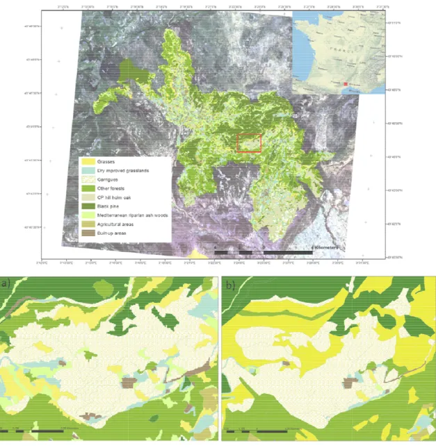
The area of investigation known as the “Foothills of Larzac” comprises a Natura 2000 sitelo-cated in the French Mediterranean BGR and covering an area of 5310 ha. It ispart of southern Massif Central, between Millau (Aveyron) and Lodève (Hérault) (Central coordinates: 3°24'29'' E; 43°45'56'' N-Figure 8). This site is characterized by the presence of limestone plateaus, locally called Causses. The elevation ranges between a minimum of 450 meters and a maximum of 820 meters. The richness of the site is related to the combination of two influ-ences: an influence of the “GrandsCausses” and a Mediterranean influence. Deep cuts in the edge of the plateau create situations that allow the development of beech (Fagussylvatica) on the Mediterranean side. The waters seeping into the limestone and dolomite of the plateau are
9 blocked by impermeable marls. On their tops many karst springs exist allowing the develop-ment of luxurious vegetation and orchids. The foothills of the Larzac area are also a sanctuary to rare plants, associated withvery specific vegetation ofsprings or seeps developing on wet carbonate materials from limestone deposits. These deposits are often low in nutrients and highly carbonated hence limiting the growth rate of plants. The floristic composition is quite diverse and often dominated by very specialized bryophytes. The main habitats of community interest present on this site are:
• Semi-natural dry grasslands and scrubland facies on calcareous substrates (6210 for Natura 2000 code and 34.31 to 34.34 for Corine biotope code). These include primary dry grasslands of the Xerobromion as well as secondary semi-dry grasslands (Meso-bromion grasslands with Bromus erectus) result of extensive grazing or mowing. The latter are mostly orchid-rich and are susceptible to shrub encroachment after the aban-donment of land use activities. The site is mainly characterized by subtype 34.332 corresponding to Middle European Xerobromion grasslands.
• Extensively managed hay meadows of the planar to submountain zones (6510 for the Natura 2000 code and 38.22 for Corine biotope code). According to the interpretation manual of European Union Habitats (European Commission DG Environment 2007), this habitat corresponds to species-rich hay meadows on little to moderately fertilised soils of the plain to submontane levels, belonging to the Arrhenatherion and the
Bra-chypodio-Centaureionnemoralis alliances. These extensive grasslands are rich in
flowers.
• Mediterranean riparian ash woods (92A0 for the Natura 2000 code and 44.63 for Co-rine biotope code). Riparian galleries dominated by tall Fraxinusangustifolia, mostly characteristic of less eutrophic soils than the (Alnus )and poplar (Populus) galleries, and of drier stations, with shorter inundation periods, than those occupied by poplar
10 woods (Aparicio Martinez, Silvestre Domingo, and Junta de Andalucía. Agencia de Medio Ambiente 1987).
The sustainability of these habitats is threatened by the change in anthropogenic activities such as land abandonment (reduction of grazing activities). It is also very much dependent on the physical and chemical properties of the water and its flow. A decrease or an interruption in the water flow may result in the extinction of the vegetation communities or to their de-cline at the benefit of less specialized vegetation species.
3.2 Datasets
3.2.1 Remote sensing
The remote sensing data comprise of two RapidEye images acquired on 23 June 2009 and 08 July 2010 (RE2009, RE2010) in the frame of Geosud project. The project offers online free
access to develop homogeneous and up-to-date spatial information on French ecosystems and territories. These images are part of two complete and consistent coverage of the French terri-tory at a very high spatial resolution. A complete coverage for 2011 is currently under pro-duction. Hence, we consider that the methodology developed on our pilot site could serve as a basis for an approach that is transferable across the 48 Natura 2000 listed sites located in the French Mediterranean BGR and covered by multi-date RapidEye data.
The images have a spatial resolution of five meters and comprise five spectral bands: Blue (b1=B); Green (b2=G); Red (b3=R); Red Edge (b4=RE) andNear infrared (b5=NIR). They were delivered in 25 km large orthorectified blocks.
For each image, the Normalized Difference Vegetation Index (NDVI) was calculated and used as a surrogate for vegetation productivity.
11
3.2.2 Elevation data
A variety of hypotheses have been proposed to account for the high diversity in the spatial distribution of natural and semi-natural habitats (Hubbell et al. 2001), and one explanation has to do with local variations in topography. Elevation data plays a crucial role in many spe-cies, habitat and niche suitability modelling studies (Mücher et al. 2009). In this study, eleva-tion data has been integrated with remote sensing data for its potential influence on the spatial distribution of the habitats present in the study area. Although we agree that other environ-mental variables influence the spatial distribution of the habitats such as soil type, we prefer to use terrain related gradients that can be widely available and hence facilitate easy transfe-rability of the method. Besides, on our pilot site, soil maps were not accessible at a scale of 1/25 000 or better. A Digital elevation model (DEM) with 25-meter grid cells provided by IGN, the French geographic institute, was used. The DEM served as a basis for the calcula-tion of the Topographic Posicalcula-tion Index (TPI). This index is a flexible way to define the rela-tive position of a location along a topographic gradient (ridge top, middle slope or valley) (Guisan, Weiss, and Weiss 1999). The TPI is simply the difference between a cell elevation value and the average elevation of the neighborhood around that cell. Positive values mean the cell is higher than its surroundings while negative values mean it is lower (Jenness 2006). The TPI is very much scale-dependent. Scale is determined by the neighborhood used in the analysis. For our study, several experiments with different windows radii showed that two circular windows sizes with a radius of five and 25 meters respectively showed the most rea-listic representation of the variations in local topography.
3.2.3 Reference data on habitats distribution
The SPLSDA method used in this study belongs to the family of supervised classification algorithms. In the supervised classification framework, the classifier (e.g. Nearest neighbor or maximum likelihood algorithms) needs to be trained using a sample of homogeneous areas
12 that can be identified either directly on the image or using thematic products (e.g. existing maps), or derived from field visits or through the combination of both approaches. Advantag-es include the ability to specify the dAdvantag-esired information classAdvantag-es (MacAlister and Mahaxay 2009). In our case, a map of natural habitats at a nominal scale of 1/25 000 has been provided by the Conservatoire des EspacesNaturels du Languedoc Roussillon (CEN-LR). The map was elaborated in 2007 by manual photointerpretation of aerial photos complemented by field visits. The map covers the Natura 2000 site only partially, but extends beyond its boundaries allowing us to test our method not only within the limits of the Natura 2000 site but also in its surroundings. The habitats were classified according to the European Corine Biotope classifi-cation system that was developed in the 1980s and used to derive the habitats, meeting the requirements of the Habitats Directive. The data was made available in vector format. 52 ha-bitat classes were recorded in the attributes table. Some polygons were assigned with “com-plex” habitat categories that correspond to an association of several habitats. These associa-tions were expressed in the form of percentages of coverage per habitat type. Only “pure” polygons assigned to one habitat class with 100% coverage were retained in this study. Be-sides, some habitat classes corresponded to “non-vegetated” areas such as built-up or water surfaces and others to agricultural areas (e.g. orchards, vineyards, etc.). In this study, only habitat classes that correspond to non-agricultural vegetation classes with a minimum area of 1 ha were considered. Finally, from the initial 52 habitat classes, 15 classes were used for the sample selection (Table 1).
[Table 1]
For each of the 15 habitat classes, half of the total polygons assigned to one specific class has been used for calibrating the SPLSDA algorithm (training set) and the other half for evaluat-ing the quality of the predicted classes (evaluation set).
13
3.3 Methodological framework
In this section, we detail the sequence of procedures used in the preparation of the data, in-cluding image analysis, for their subsequent integration into the SPLSDA algorithm. All the methods were implemented in R statistical software (mixomics package for the SPLSDA and mvoutlier for the multivariate outlier analysis).
3.3.1 Image segmentation
The method was implemented in an object-oriented image analysis framework. Unlike pixel-based approacheswhich only use the layer pixel values, the object-pixel-based techniques can also use shape, texture and other types of information supplied by ancillary data (Bock, Xofis, et al. 2005). This is relevant to the problem of distinguishing ecologically meaningful habitat types which do not have necessarily very distinct spectral features. In addition, object-oriented techniques reduce high spatial frequencynoisepresentinvery high resolution images-byexploitingthespectralandspatialdependencyof neighboring pixels, in the form of objects, and thus increasing the classification accuracy (Blaschke 2010).
Hence the first step of the method consisted in the segmentation of the remote sensing data with the purpose of generating meaningful image objects. This phase drives the next steps of variable extraction to be used in the SPLSDA algorithm. The segmentation was performed using eCognition(Definiens 2011) that allows the integration of heterogeneous datasets in the same analysis, thereby increasing the opportunity for exploiting other sources of information, not inherent to the remote sensing data, in the image classification process. All the available datasets (i.e. remote sensing data, the derived vegetation indices, elevation data) were in-gested in the same project. The RapidEye image of 08 July 2010 with its 5 spectral bands was used as a basis for the segmentation because it showed the highest contrast. In eCognition the segmentation is controlled by three parameters: scale, color (spectral information), and shape. Color and shape can be weighted jointly, each between zero to one and summing to one.
14 Within the shape setting, smoothness or compactness can be defined jointly, each betweenze-ro to one, and summing to one. Scale is a unit-less parameter that contbetweenze-rols the size of image objects, with a larger scale parameter resulting in larger image objects. Several experiments were necessary to decide on the appropriate parameters for image segmentation which can give the smallest possible number of image objects whilst providing homogenous objects in terms of the targeted habitat classes. Homogeneity in this case refers to smaller within-object than between object variance (Laliberte, Fredrickson, and Rango 2007). The following para-meters gave the best segmentation results: colour= 0.8, shape= 0.2, compactness= 0.1, smoothness= 0.9, scale = 10. Prior to the next variable extraction step, urban and agricultural areas were masked out from ancillary data. The information on urban areas was provided by the IGN (BD Topo) while that of agricultural areas was available through the French national Land parcel identification system (RPG). By masking these areas, we were able to obtain image objects that correspond only to natural vegetation.
3.3.2 Variable extraction
The image objects obtained from the segmentation can be characterized by features of differ-ent origin such as spectral values, texture, shape, context relationships and thematic or conti-nuous information supplied by ancillary data. The next step consisted of extracting features for each image object falling within a class of habitat from the reference map on habitats. Hence for each of the 15 classes of habitats, image objects falling within this class were se-lected and defined by several features. Object features can number in the 100s, because they are calculated for each layer: in this case on the five spectral bands as well as on the NDVI for the two REye images in 2009 and 2010 (NDVI2009 , NDVI2010) in addition to the TPI at
five and 25 meters (TPI5 ,TPI25). We excluded shape features such as area, width to length
ratio, shape index, and border length of image objects. Such shape features can be very useful in urban image analysis (Thomas, Hendrix, and Congalton 2003), but natural vegetation
cov-15 er in our study area is better defined by spectral and textural features. Textural features in eCognition are calculated on the gray level co-occurrence matrix (GLCM) and the gray level difference vector (GLDV) of the object pixels, after Haralick et al. (1973). The GLDV is the sum of the diagonals of the GLCM. It counts the number of references to the neighboring pixels’ absolute differences (Definiens 2011), and has shown to be useful in vegetation classi-fications (Laliberte, Fredrickson, and Rango 2007). A total of 98 object features were calcu-lated and used as variables for input to the SPLSDA (Table 2).
[Table 2]
3.3.3 Multivariate outlier analysis
For each of the 15 habitat classes, image objects falling within a habitat class, were selected as samples to be used partly for training and partly for validating the SPLSDA. The total number of sample image objects N was around 2500. These samples were derived from the reference habitat map which was generated through field visits and photointerpretation of aerial imagery in 2007. Several quality issues can be associated with this map such as i) the subjectivity of the photointerpreters in the delineation of homogeneous patches of habitat on the aerial photos, ii) the possible changes between 2007 and the image acquisition dates in 2009 and 2010 and iii) the differences between remote sensing and in-situ habitats observa-tions, each measuring different aspects of the same reality (e.g. indirect vs. direct observation techniques, differences in the spatial resolutions, differences in the typologies and in the defi-nition of homogeneous objects). These quality issues associated with the use of such a large sample increase the possibility of having some isolated outliers but also some groups of sam-ples that differ from the rest within the training set. In the context of PLS, the influence of outlier samples is clearly recognized (P. Filzmoser et al. 2009). It is hence recommended to establish if a test sample is similar enough to those used in training, otherwise the model
16 should not be applied. The possibility of detecting samples whose predictor variables consti-tute an abnormal vector (different from those of training) guarantees in some sense a kind of robustness against abnormal data in the predictor variables (Lletí et al. 2005). In this study, we used an established method for detecting multivariate outliers with robustly estimated Mahalanobis distance and QQ-plot (Gnanadesikan 1977). For a multivariate vector X, the squared Mahalanobis distance between an observation and the sample mean vector is:
/0 = 0− 1 ′34(
0− 1 (Eq.2)
where 1 is the mean and S is the covariance matrix. We can then define a multivariate outlier as a case with a large squared Mahalanobis distance. On a multivariate normal quantile plot, these cases would appear as points in the upper right that are substantially above the line for the expected χ2quantiles. We used an interactive version of this method based on a multiva-riate trimming procedure to calculate squared distances that are not affected by potential out-liers (Peter Filzmoser, Garrett, and Reimann 2005). On each iteration, some observations with the largest / values are cutoff interactively. From the remaining observations, a
trimmed mean and a trimmed covariance matrix are computed. The effect of trimming is that observations with large distances do not contribute to the calculations for the remaining ob-servations. Using the trimmed mean vector and covariance matrix, outliers will appear as points in the upper right that are substantially above the line for the expected χ2quantiles. The analysis was done using mvoutiler package available in R statistical software.
3.3.4 Variable selection and classification with SPLSDA
Given the large number of habitat classes to identify (15 classes in total) and the difficulty in interpreting the visual and numerical results of the SPLSDA, the analysis of the sample data-set was conducted through a stepwise procedure. In a first step, the samples were grouped into three broad physiognomic categories of vegetation: a “Garrigue” group including all
ha-17 bitats that correspond to low, soft-leaved scrubs (31.812, 32.11, 32.64, 32.162, 32.A); a “Grasses” group including habitats with a herbaceous vegetation cover mainly composed of graminea (34.332, 34.36, 34.721, 38.22, 81.1) and a “Forest” group representing habitats with a high density of trees (41.714, 41.9, 42.67, 44.63, 45.313). Such a grouping of habitat classes is based on the hypothesis that physiognomic characteristics of vegetation can be rea-dily distinguished in remote sensing data due to the signature of the dominant communities. Then the SPLSDA analysis is run sequentially on each of the three groups of habitats to ana-lyze the within-group separability and to see which classes of habitats can be considered sep-arately from the rest of the physiognomic group. This stepwise analysis has several advantag-es: it allows handling the large number of classes through a progressive identification of se-parable habitat classes and most of all it improves the computational time of the standard SPLSDA schema.
At each step + was set to − 1 where is the number of classes. For selecting the number of
variables ,-- to keep on each dimension, we plotted the mean classification error rate (10-cross-validation averaged 10 times) for each SPLSDA dimension. The stabilization of the estimated error rate is an indication on the optimal number of variables to be selected.
Once the most discriminant variables have been selected, the final classification has been obtained by running the SPLSDA model on all image objects resulting from the segmentation and falling within the area of investigation. The accuracy of the map of predicted habitat classes was finally analyzed using the evaluation set (see section 3.2.3).
4. Results and discussion
In this section we focus on the results of the multivariate outlier analysis and the stepwise SPLSDA that represent the main contributions of this work.
18
4.1 Detection of outliers in the sample dataset
The multivariate outlier analysis can only be applied for habitat classes with a large sample size(n >> p). Hence only classes 32.A (n = 248), 41.714 (n =550), 42.67 (n =420), 44.63 (n =247), 45.313 (n =252) were analyzed for detecting possible outliers. The multivariate outlier plots displayed in were obtained for the samples of habitat class 32.A. The left figure is the QQ-plot before the removal of outliers while the right figure is the final result after the itera-tive removal of all outliers. Outliers show up as points on the upper right side of the plot for which the Mahalanobis distance is notably greater than the χ2quantile value. Once the outliers have been removed, the distribution of the samples resembles more to a straight-line and the Mahalanobis distance between them is considerably reduced. In total 48 outliers were de-tected and removed from the original sample for habitat class 32.A. The analysis was con-ducted in the same way for the other habitat classes with large samples. Finally, 87 outliers were detected in class 41.714, 110 in class 42.67, 67 in class 44.63 and 81 in class 45.313.
[Figure 1]
4.2 Stepwise SPLSDA analysis
4.2.1 Analysis by physiognomic group
The SPLSDA was run separately on each physiognomic group of vegetation (“Garrigues”, “Grasses” and “Forest”). Given that each group consisted of 5 habitat classes, H was set to 4
( − 1) and the number of variables KeepX to select on each dimension was determined
through the analysis of the average mean classification error rate (Ten cross-validations) for each SPLSDA dimension (Figure 2). For the “Garrigues” group (Figure 2a), the error rate does not stabilize even with four dimensions. Besides, the lowest error rate of 0.42 is observed for 55 selected variables (more than half of the total number of variables used as input to the SPLSDA). The analysis of the error rate suggests that it is very difficult to differentiate
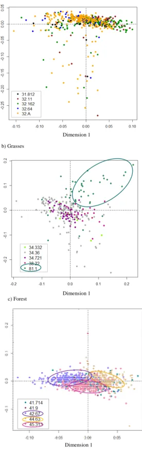
19 among them the classes of habitats of the “Garrigues” group. This is confirmed by Figure 3a which represents the samples by habitat type, within the “Garrigues” group, as a function of the latent variables selected by the SPLSDA. We represent here only the variates (1 and 4) that display the most evident dissimilarities between the samples. The latter show a strong clustering independently of the habitat class to which they belong to, thus confirming the need to group all these samples into one single class (class “Garrigues”). Inversely, the mean error rate of the “Grasses” group shows a relatively low value of 0.32 for only 2 selected va-riables on 4 dimensions (Figure 2b). These parameters were hence used to run the SPLSDA model on the “Grasses” group. The result is illustrated in Figure 3b using the first and the fourth variate. The isolation of class 81.1 from the rest of the habitats of the “Grasses” group as shown in Figure 3b indicates that this class can be analyzed and classified separately. Likewise, a relatively low error rate of approximately 0.37 is observed for the “Forest” group with 9 selected variables on 4 dimensions. Besides, the stabilization of the error rate with 4 dimensions suggests that reducing the subspaceto the first k- 1 dimensions is sufficient to explain the covariance structure of the sample data in the “Forest” group.The subspaceis de-fined by the (single) unit vector that maximizes the squared sample correlation between the response Y and the linear combination of X.
[Figure 2] [Figure 3]
Accordingly, these parameters (H= 4 and keepX= 9) were used to run the SPLSDA model on the samples of the “Forest” group. Figure 3c shows the distribution of the samples on the first and fourth SPLSDA dimensions and gives evidence of the possibility of discriminating classes 42.67, 44.63 and 45.313 from the rest of the classes. Oppositely, the samples of class 41.714 (white oak) seem to be very scattered with some samples falling in the clusters of classes 42.67, 44.63 and 45.313. According to the botanists from the CEN-LR, the white oak
20 species is ubiquitous and can grow both in the foothills and on the plains. In addition, white oak trees are present in the form of mosaics within habitat classes 44.63 and 45.313 which is clearly reflected in the samples distribution in Figure 3c.
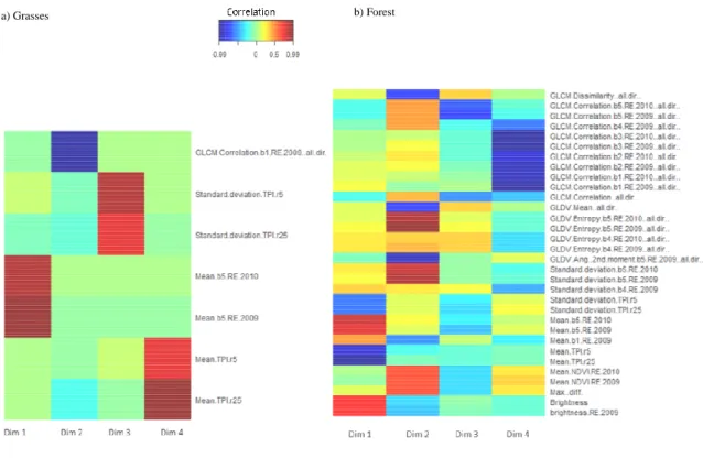
Figure4 a and b provide a closer look on the variables selected by the SPLSDA for the “Grasses” and the “Forest” physiognomic groups respectively. The heat maps of the selected variables by the SPLSDA were obtained by computing the correlations between the original data sets and the scores vectors or latent variables. The most discriminant variables are hence identifiable by high positive (dark red) or negative (deep blue) correlation values. From Fig-ure 4a, we can deduct that the NIR bands of RapidEye images in 2009 and 2010 and the TPI5
and TP25 allowed the discrimination of class 81.1 (Dry improved grasslands). The NIR band
is sensitive to dry matter; thus it is realistic to expect the selection of this variable for the dis-crimination of dry improved grasslands. Besides, according to the field experts, improved grasslands occur predominantly on plains of low elevation. This explains the selection of the topographic variables (TPI5 and TP25) by the SPLSDA for the discrimination of class 81.1.
From Figure 4b, we can deduct that several spectral variables (e.g. brightness, NIR) but also textural (e.g. GLCM correlation) and topographic variables (e.g. TPI5 and TP25) were
neces-sary for the discrimination of classes 42.67, 44.63 and 45.313. These results are also in-line with several studies that demonstrated the usefulness of textural measures for the classifica-tion of tree species (Kim and Hong 2008). Besides, riparian ash woods are likely to be lo-cated in locally lower elevations, thus explaining the selection of the topographic variables by the SPLSDA.
[Figure 4]
4.2.2 Analysis on the final habitat classes
The previous SPLSDA analysis gave insight into the similarities and the differences between habitats classes with comparable physiognomic characteristics. It also showed that the
origi-21 nal grouping of the classes of habitats needs to be reconsidered by excluding class 81.1 from the “Grasses” group and classes 42.67, 44.63 and 45.313 from the “Forest” group and consi-dering them separately in the final classification. Therefore the next step consisted in running the SPLSDA analysis with the new set of habitats classes: “Garrigues” (comprising classes 31.812,32.11, 32.64, 32.162 and32.A),“Grasses” (comprising classes 34.332, 34.36, 34.721 and 38.22), Improved grassland (class 81.1.), Black pine (class 42.67),Mediterraneanriparianashwoods(class44.63),Catalo-Provencal (CP) hill holm-oak (class 45.313) and “Other forests” (comprising classes 41.714 and 41.9). To decide on the number of variables to retain for the final classification, we run the SPLSDA with different dimensions and an increasing number of selected variables. In Figure 5 the mean classifica-tion error rate is shown for each SPLSDA dimension and a selected number of variables. These results show that at least 4 dimensions are needed to discriminate the 7 classes of habi-tats. The error rates on dimensions five and six show parallel variations, and are sometimes equivalent on dimensions 6 and 7. The minimum error rate of 0.31 is obtained on dimension 7 with 16 selected variables and on dimension 6 with 35 variables. If we set the maximum acceptable error rate to 0.32, then it is sufficient to set H to 6 dimensions and the number of variables to choose on each dimension keepX to 4. Those criteria were selected for running the final SPLSDA model with the purpose of predicting the classes of habitats over the entire study area.
[Figure 5] [Figure 6]
Figure 6 shows the samples of the 7 final habitat classes represented by the values of their loading vectors computed on dimensions one and four (left) and dimensions three and six (right). The first and fourth dimensions of the SPLSDA allow the discrimination of dry im-proved grasslands, black pine, oak woodland and riparian ash woods. They fail at
discrimi-22 nating the “Grasses” group and the “Garrigues” group that are almost invisible on the left figure. On the contrary, the third and the sixth dimensions seem to better differentiate the “Grasses” and “Garrigues” groups while the classes of oak woodland and black pines seem to be more scattered on the same dimensions. As already noticed in the previous analysis, the group “Other Forests” shows a less evident clustering and spreads over the other classes of forest habitats (i.e. oak woodland, riparian ash woods and black pine).
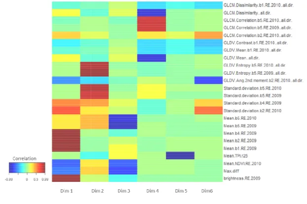
The selected variables that strongly contribute to the discrimination of the seven classes of habitats are shown in Figure 7 and are highlighted by high correlation values with the latent variables. We notice that the variables that mostly contribute to the separation of the habitats are essentially the spectral features of the RapidEye images in 2009 and 2010 (e.g. Mean, brightness and STD) as well as the textural features mainly in the NIR bands of the two im-ages. Curiously, the features derived from the NDVI and the Red band were rarely selected by the SPLSDA and seem to be less important for the discrimination of the habitat classes present in the study area. Temporal variations of the NDVI could help in distinguishing im-proved grasslands when the NDVI is calculated from different observation dates in the annual cycle (Lucas et al. 2007). The two RapidEye images used in our analysis were acquired dur-ing the summer season of 2009 and 2010. Usually, year to year reflectance of the landscape should be relatively similar in the summer period as many vegetation coversare close to max-imum production. This possibly explains the lack of significant contribution of the NDVI to the discrimination of the habitat classes.
[Figure 7]
4.3 Map output and accuracy assessment
The SPLSDA model defined on a subset of variables was then used for predicting the habitats over the full study area. This stage consists in assigning a class of habitat from the seven final habitat classes to each image object resulting from the image segmentation of the remote
23 sensing data. The map resulting from the application of the SPLSDA model is represented in Figure 8. An enlarged part of the mapping is provided in Figure 8a exemplifying the level of detail achieved. Compared to the CEN-LR map resulting from photointerpretation of aerial imagery (Figure 8b), the classification using RapidEye imagery and the SPLSDA approach provides a more detailed delineation of the main habitat classes. However, from the initial 52 habitat classes (including non-vegetated and agricultural classes), the method was successful in distinguishing only seven classes. These performances could be considered as acceptable for reporting obligations in the framework of the Habitats Directive which focus on the cha-racterization of the spatial distribution and the total area of specific habitats of community interest.
[Figure 8]
To assess the accuracy of the habitats map, the evaluation set derived from the CEN-LR map was used (section 3.2.2). It consisted of 1024 image objects classified according to the 15 initially retained habitat classes. The latter had to be regrouped into seven classes to allow their comparison with the classification output and for computing the confusion matrix (Erreur ! Source du renvoi introuvable.). The accuracy of classification was assessed using three quality indicators derived from the confusion matrix: the overall, the user's (u) and the producer's (p) accuracies.
[Table 3]
The overall accuracy (71%) of the map, although not very high can be considered as satisfac-tory in the particular context of the study area, characterized by the complexity and the hete-rogeneity of its habitats. The highest user accuracy was obtained for dry improved grasslands (u=91.97%) followed by riparian ash woods (u= 88.38%). These results are very encouraging given that these two classes were identified in Annex 1 of the EC Habitats Directive as of community interest. Classes that were less well predicted were “Garrigues” (u= 58%, p=
24 79%), Catalo-Provencal hill holm-oak woodland (u= 36%, p= 69%) and “Other forests” (u= 49%, p= 63%). The classes are found typically in complex arrangements of vegetation mo-saics (mainly for “Garrigues” and “Other forests”). They are also regarded as broadly defined and contain many different types of vegetation communities (e.g. “Garrigues”). Some quality issues associated with the use of the CEN-LR map as a reference for validation need to be considered here: although only pure habitat classes (with a percentage of coverage of 100%) were used as a reference for validation, a majority of the image objects derived from the CEN-LR map contained a mix of vegetation types. This is particularly well illustrated for class 41.714 which is very ubiquitous and spread across other forest tree species. A field visit to the study area accompanied by an experienced ecologist confirmed the tendency of the photointerpreters or the field surveyors to give different priorities to the various components of the observed habitat patches,resulting in different extents of these habitats. For this reason, the results of the accuracy assessment presented here should be interpreted with caution. Pro-viding more consistent delineations of habitats and definitions of vegetation types would re-duce the uncertainties both in the training and in the evaluation sets. A solution to be consi-dered is the use of an automatic segmentation of remote sensing data that can ensure consis-tency and can help reducing the amount of time spent in the visual interpretation and the digi-tization of aerial photos.
5. Conclusion and outlooks
This study investigated the use of a relatively new multivariate exploratory approach, the SPLSDA, for the classification of natural and semi-natural Natura 2000 habitats from remote sensing data. Several benefits to the approach can be highlighted:
• The SPLSDA approach is very well suited for the analysis and classification of re-mote sensing data in general and for predicting habitat classes in particular. It includes
25 a built-in variable selection procedure that allows avoiding collinearity and that can remove unnecessary predictors that add noise to the estimation. This is of particular interest in high dimensional multi-class classification problems as in the case of de-tailed classification of Natura 2000 habitats with multi-spectral and multi-date remote sensing data.
• The SPLSDA approach selected relevant and stable variables for the discrimination of habitat classes that could be linked to ecological or biophysical characteristics. The variables selected by the SPLSDA can serve as indicators for feature selection if a standard nearest neighbor classification was to be used. Besides, these variables can also guide the implementation of decision rules, if a rule-based classification, similar to that proposed by Lucas et al.(2007) was to be developed.
• 7 Habitat classes were identified and classified by the approach with an overall accu-racy of 71% including two habitats of community interest (Mediterranean riparian ash woods and dry improved grasslands). To achieve this level of accuracy, only two Ra-pidEye images were required and a DEM with 25 meter grid cells demonstrating the ease of implementation of the method and its update at a reasonable cost and with li-mited technical constraints. Due to lili-mited data input requirements and to its compu-tational efficiency, the SPLSDA i) is a good alternative to other types of variable se-lection approaches in a supervised classification framework and ii) can be easily transferred to other Natura 2000 sites.
For achieving better results in terms of discrimination of a larger number of habitat classes, it is necessary to improve the learning stage of the SPLSDA model. This can be at-tained through the use of more adequate reference data (e.g. field data tailored to the classifi-cation of remote sensing imagery or photointerpretation of homogeneous image objects re-sulting from an automated segmentation of the remote sensing data). Despite the beneficial
26 effect of outliers’ detection and removal thanks to the multivariate outlier analysis, the refer-ence data still includes heterogeneous areas and ill-defined habitats. In addition to the en-hancement of the learning set, a special effort should be dedicated for redefining the typolo-gies of habitats and for establishing a relationship between the classes of habitats in the field and biophysical parameters that can be accessible through remote sensing.
Other data sources could be also tested and included in the SPLSDA analysis for discri-minating a larger number of habitat classes. If available, thematic information on soil proper-ties can be beneficial for the discrimination of Xerobromion grasslands that occur naturally on shallow calcareous soils where no forest growth is possible. Multiseasonal remote sensing data can be also very useful for detecting trends in the NDVI that may help in distinguishing between combinations of vegetation types e.g. improved and semi-improved grasslands) and mainly between coniferous (e.g. Black pine), other evergreen (e.g. holm-oak) and deciduous forest species (e.g. white oak). As recommended by Lucas (2011), multiseasonal image ac-quisitions ought to occur when contrasts inthe spectralreflectanceorassociatedcharacteristic-sof vegetationare exaggeratedandcanbecaptured. Specifically, the need for early spring im-agery before the leaf flush was highlighted as, for many habitats (e.g. broadleaved wood-lands) substantial contrasts with their reflectance in the post-spring period were observed which facilitate their discrimination.
The wider application of the method requires: i) access to suitable reference data on exist-ing habitats, ideally, based on photointerpretation and ground-truthexist-ing by an experienced ecologist, ii) the availability of very high resolution imagery with NIR band as a primary source for segmenting the landscape into homogenous image objects that reflect the habitat patterns and iii) the availability of ancillary data (e.g DEM) that would lead to further en-hancement of the classification of the habitats. As such, the mapping approach proposed here has application on other Natura 2000 sites. It has been successfully applied on Lagoons of
27 Palavas site characterized by the coexistence of different coastal habitats: dune systems, fore-shore and salt marshes. Multi-date Worldview-2 imagery, together with colour infrared aerial photos and a Digital Surface Model were used as an input to the SPLSDA. In a future study, we intend to apply the approach on two new sites, the Aude valley (Mediterranean BGR) and Belledonne plain (Alpine BGR) and to compare our results with those of nearest neighbor and rule-based approaches.
6. References
Aparicio Martinez, Abelardo, Santiago Silvestre Domingo, and Junta de Andalucía. Agencia de Medio Ambiente. 1987. Flora del Parque Natural de la Sierra de Grazalema. Sevilla: Junta de Andalucía, Agencia de Medio Ambiente.
Barker, Matthew, and William Rayens. 2003. “Partial Least Squares for Discrimination.”
Journal of Chemometrics 17 (3) (March 24): 166–173.
Blaschke, T. 2010. “Object Based Image Analysis for Remote Sensing.” ISPRS Journal of
Photogrammetry and Remote Sensing 65 (1) (January): 2–16. Bock, Michael. 2003.
“Remote Sensing and GIS-based Techniques for the Classification and Monitoring of Biotopes: Case Examples for a Wet Grass- and Moor Land Area in Northern Ger-many.” Journal for Nature Conservation 11 (3): 145–155.
Bock, Michael, Godela Rossner, Michael Wissen, Kalle Remm, Tobias Langanke, Stefan Lang, Hermann Klug, Thomas Blaschke, and Borut Vrščaj. 2005. “Spatial Indicators for Nature Conservation from European to Local Scale.” Ecological Indicators 5 (4) (November): 322–338.
Bock, Michael, Panteleimon Xofis, Jonathan Mitchley, Godela Rossner, and Michael Wissen. 2005. “Object-oriented Methods for Habitat Mapping at Multiple Scales – Case Stud-ies from Northern Germany and Wye Downs, UK.” Journal for Nature Conservation 13 (2-3): 75–89.
Boulesteix, Anne-laure. 2004. “PLS Dimension Reduction for Classification with Microarray Data.” In Statistical Applications in Genetics and Molecular Biology 3, Issue 1,
Arti-cle 33, 1–33.
Lê Cao, Kim-Anh, Simon Boitard, and Philippe Besse. 2011. “Sparse PLS Discriminant Analysis: Biologically Relevant Feature Selection and Graphical Displays for Multi-class Problems.” BMC Bioinformatics 12 (1): 253.
Lê Cao, Kim-Anh, Pascal GP Martin, Christèle Robert-Granié, and Philippe Besse. 2009. “Sparse Canonical Methods for Biological Data Integration: Application to a Cross-platform Study.” BMC Bioinformatics 10 (1): 34.
Chun, Hyonho, and S. Keles. 2010. “Sparse Partial Least Squares Regression for Simultane-ous Dimension Reduction and Variable Selection.” Journal of the Royal Statistical
Society: Series B (Statistical Methodology) 72 (1) (January): 3–25.
Chung, Dongjun, and Sunduz Keles. 2010. “Sparse Partial Least Squares Classification for High Dimensional Data.” Statistical Applications in Genetics and Molecular Biology 9 (1) (January 3): 1–30.
28 Consonni, Viviana, DavideBallabio, and Roberto Todeschini.2010. “Evaluation of Model Predictive Ability by External Validation Techniques.” Journal of Chemometrics 24 (3-4) (February 17): 194–201.
Definiens. 2011. “Definiens, 2011: eCognition 4 User Guide”. Definiens Documentation. Munich.
Díaz Varela, R., P. Ramil Rego, S. Calvo Iglesias, and C. Muñoz Sobrino. 2008. “Automatic Habitat Classification Methods Based on Satellite Images: A Practical Assessment in the NW Iberia Coastal Mountains.” Environmental Monitoring and Assessment 144 (1): 229–250.
European Commission DG Environment. 2007. “Interpretation Manual of European Union Habitats.” EUR 27. Brussels: European Commission, DG Environment.
Filzmoser, P., S. Serneels, R. Maronna, and P.J. Van Espen. 2009. “Robust Multivariate Methods in Chemometrics.” In Comprehensive Chemometrics, 681–722. Elsevier. Filzmoser, Peter, Robert G. Garrett, and Clemens Reimann. 2005. “Multivariate Outlier
De-tection in Exploration Geochemistry.” Computers & Geosciences 31 (5) (June): 579– 587.
Filzmoser, Peter, Moritz Gschwandtner, and Valentin Todorov. 2012. “Review of Sparse Methods in Regression and Classification with Application to Chemometrics.”
Jour-nal of Chemometrics 26 (3-4) (March): 42–51.
Gnanadesikan, Ram. 1977. Methods for Statistical Data Analysis of Multivariate
Observa-tions. Wiley Series in Probability and Mathematical Statistics. New York: Wiley.
Guisan, A., S. Weiss, and A. Weiss. 1999. “GLM versus CCA spatial modeling of plant spe-cies distribution.” Plant Ecology 143 (1): 107–122.
Haralick, Robert M., K. Shanmugam, and Its’Hak Dinstein. 1973. “Textural Features for Im-age Classification.” IEEE Transactions on Systems, Man, and Cybernetics 3 (6) (No-vember): 610–621.
Hubbell, Stephen P., Jorge A. Ahumada, Richard Condit, and Robin B. Foster. 2001. “Local Neighborhood Effects on Long-term Survival of Individual Trees in a Neotropical Forest.” Ecological Research 16 (5) (December): 859–875.
Jenness, J. 2006. Topographic Position Index (tpi_jen.avx) Extension for ArcView 3.x, V. 1.2. Jenness Entreprises. http://www.jennessent.com/arcview/tpi.htm.
Keramitsoglou, Iphigenia, Charalambos Kontoes, Nicolaos Sifakis, Jonathan Mitchley, and Panteleimon Xofis. 2005. “Kernel Based Re-classification of Earth Observation Data for Fine Scale Habitat Mapping.” Journal for Nature Conservation 13 (2–3): 91–99. Kerr, Jeremy T., and Marsha Ostrovsky. 2003. “From Space to Species: Ecological
Applica-tions for Remote Sensing.” Trends in Ecology & Evolution 18 (6) (June): 299–305. Kim, Choen, and Sung-Hoo Hong. 2008. “Identification of Tree Species from
High-resolution Satellite Imagery by Using Crown Parameters.” In , edited by Christopher M. U. Neale, Manfred Owe, and Guido D’Urso, 71040N–71040N–8.
Krämer, Nicole. 2007. “An Overview on the Shrinkage Properties of Partial Least Squares Regression.” Computational Statistics 22 (2) (March 9): 249–273.
Laliberte, A.S., E.L. Fredrickson, and A. Rango. 2007. “Combining Decision Trees with Hi-erarchical Object-oriented Image Analysis for Mapping Arid Rangelands.”
Photo-grammetric Engineering and Remote Sensing 73 (2): 197–207.
Lletí, R., E. Meléndez, M.C. Ortiz, L.A. Sarabia, and M.S. Sánchez. 2005. “Outliers in Partial Least Squares Regression.” Analytica Chimica Acta 544 (1-2) (July): 60–70.
Lucas, Richard, Katie Medcalf, Alan Brown, Peter Bunting, Johanna Breyer, Dan Clewley, Steve Keyworth, and Philippa Blackmore. 2011. “Updating the Phase 1 Habitat Map of Wales, UK, Using Satellite Sensor Data.” ISPRS Journal of Photogrammetry and
29 Lucas, Richard, Aled Rowlands, Alan Brown, Steve Keyworth, and Peter Bunting. 2007. “Rule-based Classification of Multi-temporal Satellite Imagery for Habitat and Agri-cultural Land Cover Mapping.” ISPRS Journal of Photogrammetry and Remote
Sens-ing 62 (3): 165–185.
MacAlister, Charlotte, and Manithaphone Mahaxay. 2009. “Mapping Wetlands in the Lower Mekong Basin for Wetland Resource and Conservation Management Using Landsat ETM Images and Field Survey Data.” Journal of Environmental Management 90 (7) (May): 2130–2137.
Mücher, Caspar A., Stephan M. Hennekens, Robert G.H. Bunce, Joop H.J. Schaminée, and Michael E. Schaepman. 2009. “Modelling the Spatial Distribution of Natura 2000 Habitats Across Europe.” Landscape and Urban Planning 92 (2) (September 15): 148–159.
Nagendra, H. 2001. “Using Remote Sensing to Assess Biodiversity.” International Journal of
Remote Sensing 22 (12) (January 1): 2377–2400.
Nagendra, Harini, Richard Lucas, JoãoPradinhoHonrado, Rob H.G. Jongman, Cristina Taran-tino, Maria Adamo, and Paola Mairota. 2012. “Remote Sensing for Conservation Monitoring: Assessing Protected Areas, Habitat Extent, Habitat Condition, Species Diversity, and Threats.” Ecological Indicators (October).
Shen, Haipeng, and Jianhua Z. Huang. 2008. “Sparse Principal Component Analysis via Regularized Low Rank Matrix Approximation.” Journal of Multivariate Analysis 99 (6) (July): 1015–1034.
Thomas, N.a, C.a Hendrix, and R.G.b Congalton. 2003. “A Comparison of Urban Mapping Methods Using High-resolution Digital Imagery.” Photogrammetric Engineering and
Remote Sensing 69 (9): 963–972.
Turner, Woody, Sacha Spector, Ned Gardiner, Matthew Fladeland, Eleanor Sterling, and Marc Steininger. 2003. “Remote Sensing for Biodiversity Science and Conservation.”
Trends in Ecology & Evolution 18 (6) (June): 306–314.
Vanden Borre, J., B. Haest, S. Lang, T. Spanhove, M. Forster, and N.I. Sifakis. 2011. “To-wards a Wider Uptake of Remote Sensing in Natura 2000 Monitoring: Streamlining Remote Sensing Products with Users’ Needs and Expectations.” In Proceedings, 2nd
International Conference on Space Technology (ICST), 1–4.
Weiers, Stefan, Michael Bock, Michael Wissen, and Godela Rossner. 2004. “Mapping and Indicator Approaches for the Assessment of Habitats at Different Scales Using Re-mote Sensing and GIS Methods.” Landscape and Urban Planning 67 (1–4) (March 15): 43–65.
Wolter, P, P Townsend, B Sturtevant, and C Kingdon. 2008. “Remote Sensing of the Distri-bution and Abundance of Host Species for Spruce Budworm in Northern Minnesota and Ontario.” Remote Sensing of Environment 112 (10) (October 15): 3971–3982.
30 Table 1.The main natural habitats existing in the Foothills of LarzacNatura 2000 site of Foo-thills of Larzac. Each class of habitat is assigned a code according to the European Corine Biotope classification system that was developed in the 1980s and used to derive the habitats, meeting the requirements of the Habitats Directive.
31.812 Blackthorn-privet scrub
38.22
Medio-European lowland hay mea-dows
32.11 Evergreen oak matorral 41.714 Eu-Mediterranean white oak woods 32.162 Western deciduous oak matorral 41.9 Chesnut woods
32.64 Supra-Mediterranean box scrub 42.67 Black pine reforestation
32.A Spanish-broom fields 44.63 Mediterranean riparian ash woods 34.332 Middle European xerobromion
grasslands
45.313 Catalo-Provencal hill holm-oak
34.36 Phoenician torgrass swards 81.1 Dry improved grasslands 34.721 Aphyllanthes grasslands
31 Table 2.Summary table of the main object features used as variables for input to the
SPLSDA. All spectral and textural features were computed on both RapidEye images ac-quired in 2009 and 2010.
Spectral Category Feature Definition
Layers values Mean Mean values of image object in the B, G, R, RE, NIR bands STD Standard deviation of image object in the B, G, R, RE, NIR
bands
Brightness Mean of the mean values of all spectral bands of RE images Maximum
dif-ference
Difference between the maximum and the minimum mean intensity values divided by the brightness of all spectral bands Band ratios Mean NDVI Mean values of image object calculated on the NDVI
STD NDVI Standard deviation of image object calculated on the NDVI Textural GLCM Correlation Measure of the linear dependency of gray levels of
neighbor-ing pixels
Dissimilarity Measure of the amount of local variation in the image.
GLDV Second angular moment
Measure of the local homogeneity. The value is high if some elements of the GLDV are large and the remaining ones are small.
Entropy Measure of the randomness of the gray-level distribution Mean The average expressed in terms of the GLDV. The pixel value
is not weighted by its frequency of occurrence itself, but by the frequency of its occurrence in combination with a certain neighbor pixel value.
Contrast Contrast is the opposite of homogeneity. It is a measure of the amount of local variation in the image.
Thematic Topography TPI5 Topographic Position Index calculated with a radius of 5
me-ters
TPI25 Topographic Position Index calculated with a radius of 25
32 Table 3.Confusion matrix of the result of the classification using the SPLSDA model. The reference data is represented in columns and the classification outputs in rows.
Garrigues Grasses Dry improved grasslands
Black pine Riparian ash woods CP hill holm-oak Other forests Garrigues 34 5 3 3 5 5 4 Grasses 0 64 15 0 13 3 2 Dry improved grasslands 0 7 126 0 2 0 2 Black pine 3 3 3 201 17 3 14 Riparian ash woods
0 3 6 10 175 2 2 CP hill holm-oak 3 6 12 16 17 44 24 Other forest 3 8 21 20 25 7 82 Producer accuracy (%) 79.07% 66.67% 67.74% 80.40% 68.90% 68.75% 63.08% User accuracy (%) 57.63% 65.98% 91.97% 82.38% 88.38% 36.07% 49.40% Overall accuracy (%) 70.97%
33 Figure 1.Plot of the ordered robust Mahalanobis distances of the samples of habitat class 32.A against the quantiles of the χ2 distribution (left). If the data is normally distributed these values should approximately correspond to each other, so outliers can be detected visually. By user interaction this procedure is repeated, each time leaving out the observation with the greatest distance. This method can be seen as an iterative deletion of outliers until a straight line appears (right).
Ordered robust Mahalanobis distance
Q u a n ti le s of χ 2
34 Figure 2. Estimated classification error rate (Ten cross validation) with respect to the number of selected variables on each dimension of SPLSDA for the “Garrigues” (a), “Grasses” (b) and “Forest” (c) groups.
a) Garrigues
c) Forest
35 b) Grasses c) Forest Dimension 1 Dimension 1 Dimension 1
Figure 3.Sample representation using the most discriminant dimensions from the SPLSDA for the “Garrigues” (a), “Grasses” (b) and “Forest” (c) groups.
Figure 4. Heat maps of the selected variables by the SPLSDA for the «
« Forest » groups. The colors vary with the degree of correlation between the original data sets and the latent variables.
a) Grasses
Heat maps of the selected variables by the SPLSDA for the «
» groups. The colors vary with the degree of correlation between the original data b) Forest
36 Heat maps of the selected variables by the SPLSDA for the « Grasses » and the » groups. The colors vary with the degree of correlation between the original data
37 Figure 5. Estimated classification error rate (10 cross validation averaged 10 times) with re-spect to the number of selected variables on each dimension of the SPLSDA for the seven final classes of habitats.
0.3 0.35 0.4 0.45 0.5 0.55 0 5 10 15 20 25 30 35 40 45 50 A v e ra g e e rr o r ra te ( r2 )
Number of selected variables
38 Figure 6.Sample representation using the most discriminant dimensions of the SPLSDA model for the seven final classes of habitats.
X -v a ri a te 6 X -v a ri a te 4 X-variate 3 X-variate 1
Figure 7. Heat map representing the correlation values between the selected variables each of the dimensions of the SPLSDA model for the
keepX = 4).
. Heat map representing the correlation values between the selected variables each of the dimensions of the SPLSDA model for the seven final habitat classes (
39 . Heat map representing the correlation values between the selected variables and final habitat classes (H =6 and