Diversity-inducing probability measures for machine learning

Diversity-Inducing Probability Measures for

Machine Learning

by

Chengtao Li

B.S., Tsinghua University (2014)

M.S., Massachusetts Institute of Technology (2016)

Submitted to the Department of Electrical Engineering and Computer

Science

in partial fulfillment of the requirements for the degree of

Doctor of Philosophy

at the

MASSACHUSETTS INSTITUTE OF TECHNOLOGY

February 2019

@

Massachusetts Institute of Technology 2019. All rights reserved.

Author

....

Signature redacted

...

Department of Electrical Engineering and Computer Science

SiginatureAredacted

January 31, 2019

Certified by ... ...

Suvrit Sra

Assistant Professor of Electrical Engineering and Computer Science

Thesis Supervisor

Certified by.

Signature redacted...

Stefanie Jegelka

Assistant Professor of Electrical Engineering and Computer Science

f. Thesis Supervisor

Accepted by...

gnature redacted

...

MASSACHUSETTS INSTITUTE

_\'

_U

_-J

_{Leslie A. Kolodziejski}

OF

r

Professor of Electrical Engineering and Computer Science

FEB 2 12019

Chair,

Department Committee on Graduate Students

Diversity-Inducing Probability Measures for

Machine Learning

by

Chengtao Li

Submitted to the Department of Electrical Engineering and Computer Science on January 31, 2019, in partial fulfillment of the

requirements for the degree of Doctor of Philosophy

Abstract

Subset selection problems arise in machine learning within kernel approximation, experi-mental design, and numerous other applications. In such applications, one often seeks to select diverse subsets of items to represent the population. One way to select such diverse subsets is to sample according to Diversity-Inducing Probability Measures (DIPMs) that assign higher probabilities to more diverse subsets. DIPMs underlie several recent break-throughs in mathematics and theoretical computer science, but their power has not yet been explored for machine learning. In this thesis, we investigate DIPMs, their mathematical properties, sampling algorithms, and applications.

Perhaps the best known instance of a DIPM is a Determinantal Point Process (DPP). DPPs originally arose in quantum physics, and are known to have deep relations to linear algebra, combinatorics, and geometry. We explore applications of DPPs to kernel matrix approximation and kernel ridge regression. In these applications, DPPs deliver strong approximation guarantees and obtain superior performance compared to existing methods. We further develop an MCMC sampling algorithm accelerated by Gauss-type quadratures for DPPs. The algorithm runs several orders of magnitude faster than the existing ones.

DPPs lie in a larger class of DIPMs called Strongly Rayleigh (SR) Measures. Instances of SR measures display a strong negative dependence property known as negative association, and as such can be used to model subset diversity. We study mathematical properties of SR measures, and construct the first provably fast-mixing Markov chain that samples from general SR measures. As a special case, we consider an SR measure called Dual Volume Sampling (DVS), for which we present the first poly-time sampling algorithm.

While all considered distributions over subsets are unconstrained, those of interest in the real world usually come with constraints due to prior knowledge, resource limitations or personal preferences. Hence we investigate sampling from constrained versions of DIPMs. Specifically, we consider DIPMs with cardinality constraints and matroid base constraints and construct poly-time approximate sampling algorithms for them. Such sampling algorithms will enable practical uses of constrained DIPMs in real world.

Thesis Supervisor: Suvrit Sra

Title: Assistant Professor of Electrical Engineering and Computer Science Thesis Supervisor: Stefanie Jegelka

Acknowledgments

First and foremost, I am forever thankful to my advisors, Suvrit Sra and Stefanie Jegelka, for their never-ending guidance and support throughout my PhD. They have always been a strong support for me and gave me the freedom to pursue anything I want. Only with such free environment can I possibly produce any good work. This thesis would not have been possible without them - they were the best advisors that I could have ever asked for.

I am also thankful to my fantastic thesis committee member, Devavrat Shah. He is extremely nice and patient, and has given me very valuable opinions on my work. I am very fortunate to have him on my thesis committee.

Many thanks must also go to my wonderful collaborators, friends and people in my group. I have benefited tremendously from conversations with Yonatan Belinkov, Benson Chen, Hongge Chen, Connor Coley, Wengong Jin, Nate Kushman, Tao Lei, Ruizhi Liao, Ge Liu, Tianren Liu, Hongzhou Lin, Zelda Mariet, David Alvarez Melis, Evan Pu, Tianxiao Shen, Matt Staib, Zi Wang, Jiajun Wu, Keyulu Xu, Zhi Xu, Guowei Zhang, Hongyi Zhang, Jingzhao Zhang, Yu Zhang, Yuan Zhang and Xijia Zheng. I will never forget all those discussions (on any topics) with you at Stata Center, and will always miss those activities we have attended together. I also want to thank staffs at MIT for their help with all administrative things.

A big thank you to all members at MIT-CHIEF (MIT-China Innovation and Entrepreneur-ship Forum), with whom I have spent the last three wonderful years. When I joined MIT-CHIEF three years ago, I knew nothing about entrepreneurship. During these three years I have met so many fantastic people and have learned so much from them. I will never forget the days and nights when we worked together.

There are several people that I want to show my special thank for:

" Jingkai Chen, for being such a supportive friend. He always says how much he has learnt from me, but what I have learnt from him is much more. He sets a very high standard for himself. Encouraged by this, I have been trying to do the same.

" Ning Jiang, for staying with me during the first two years of my PhD, and continue to be my friend afterwards. The beginning of my PhD was a hard time for me, and I

could not sustain without her support. She has became the one who I turn to when I do not know what to do. She could point me to the correct direction with a few words. " Qingkai Liang, for being my best friend throughout my PhD. I cannot recall how many times he had helped me out. I can still remember those days and nights when we chatted and got drunk together. I became a ski lover and wine lover because of him. We even went to wine-tasting courses together and both got level-2 certificate of WSET. My PhD life would be much less awesome without him.

" Chu Ma, for countless meals and table tennis together. She is an excellent example of what a solid female researcher looks like. She is one of the very few people who I know could continue exercising almost every single day. I admire her and am encouraged by her.

" Fangchang Ma, for being such a critical friend on mouth but such a helpful friend at heart. He taught me how to view things critically and allow me to see a new form of humor. I also learnt a lot about leadership from him.

" Fanyu Que, for showing up in my life and staying close with me during the last year of my PhD. She has been bearing with my impatience and naiveness with her incredible patience and tolerance. I could act as a boy in front of her. There is countless number of times when she raised me up. I could not be luckier to have her with me.

* Dajiang Suo, for showing me how a mature man should act. I have benefitted tremendously from learning the way he talks. I feel lucky to be one of his friends. " Yunming Zhang, for being my best roommate for three and a half years, providing me

with so much help. I have to say I am not a perfect roommate, but he is always nice and patient to me. I really appreciate it.

Finally, I would like to thank my parents, Songyue and Jun, for their supports and patience to me through the entire PhD process. They always gave their strongest support whenever I do any decisions. I dedicate this thesis to my wonderful family.

Bibliographic Notes

The main ideas in this thesis have been published in peer-reviewed conferences and one preprint. The list of papers is as follows:

" Fast DPP Sampling for Nystrom with Application to Kernel Methods. Interna-tional Conference on Machine Learning (ICML), 2016.

" Gaussian Quadrature for Matrix Inverse Forms with Applications. International Conference on Machine Learning (ICML), 2016.

" Fast Mixing Markov Chains for Strongly Rayleigh Measures, DPPs, and Con-strained Sampling. Advances in Neural Information Processing Systems (NIPS),

2016

" Polynomial Time Algorithms for Dual Volume Sampling. Advances in Neural Information Processing Systems (NIPS), 2017

" Fast Mixing Markov Chains for Strongly Rayleigh Measures and Variants. In Preparation, 2018

The code for the work presented in this thesis is publicly available at https: //

Contents

1 Introduction 19

2 Determinantal Point Processes for Kernel Methods 25

2.1 Introduction . . . 25

2.2 Background and Notation . . . 27

2.3 DPP for the Nystrnm Method . . . 28

2.4 Low-rank Kernel Ridge Regression . . . 31

2.5 Experiments . . . 34

2.5.1 Kernel Approximation . . . 34

2.5.2 Kernel Ridge Regression . . . 35

2.5.3 Mixing of the Markov Chain DPP . . . 36

2.5.4 Time-Error Tradeoffs . . . 39

2.6 Summary . . . 40

3 Sampling DPP by Efficient MCMC with Gauss Quadrature 41 3.1 Bilinear Inverse Forms (BIFs) . . . . 41

3.1.1 Determinantal Point Processes (DPPs) . . . 43

3.1.2 MCMC for (k-)DPP . . . 44

3.1.3 Other Motivating Applications . . . 46

3.2 Background on Gauss Quadrature . . . 48

3.3 Main Theoretical Results . . . 54

3.3.1 Lower Bounds . . . 55

3.3.3 Convergence rates . . . . 3.3.4 Empirical Evidence . . . . 3.4 Proofs for Main Theoretical Results . . . . 3.5 Generalization: Symmetric Matrices . . . . 3.6 Algorithmic Results and Efficient (k-)DPP Sampling

3.6.1 Retrospective Markov Chain (k-)DPP . . . . 3.6.2 Empirical Evidence . . . . 3.7 Numerical details . . . . 3.8 Summary . . . .

4 Sampling from Strongly Rayleigh Measures

4.1 Introduction . . . . 4.1.1 SR Instantiations . . . . 4.1.2 Sampling using MCMC . . . . 4.1.3 Other Related work . . . . 4.2 Sampling from General Strongly Rayleigh Measures

4.2.1 Experiments . . . . 4.3 Dual Volume Sampling . . . . 4.3.1 Connections and implications. . . . . 4.4 SR Property and Fast Markov Chain Sampling . . . . 4.4.1 Strong Rayleigh Property of DVS . . . . 4.4.2 Implications: MCMC . . . . 4.4.3 Further implications and connections . . . . 4.5 Polynomial-time Dual Volume Sampling . . . . 4.5.1 Marginals . . . . 4.5.2 Sampling . . . . 4.5.3 Derandomization . . . . 4.6 Experiments . . . . 4.7 Summary . . . . 56 57 58 67 . . . 69 69 73 76 77 79 79 80 81 83 83 86 87 89 90 90 93 95 95 96 97 98 . . . . 99 . . . 100

5 Constrained Sampling

5.1 Introduction . . . . 5.2 Sampling from SR with Cardinality Constraint . . . . 5.2.1 Chain Combination for Easy Fast-Mixing Chain Construction 5.2.2 Application to Sampling from SR with Cardinality Constraints 5.3 Sampling from DIPMs with Matroid Base Constraints . . . . 5.4 Experim ents . . . . 5.5 Sum m ary . . . .

6 Conclusion and Open Problems

101 . . . 101 . . . 104 . . . 104 . . . 112 . . . 118 . . . 122 . . . 124 125 A Supplementary Experiments for Chapter 2 127 A. 1 Kernel Approximation . . . 127

A.2 Approximated Kernel Ridge Regression . . . 127

A.3 Mixing of Markov Chain k-DPP . . . 127

A.4 Running Time Analysis . . . 128

B Supplementary Proofs and Experiments for Chapter 4 135 B.1 Partition Function . . . 135

B.2 Marginal Probability . . . 137

B.3 Approximate Sampling via Volume Sampling . . . 141

B.4 Conditional Expectation . . . 144

B.5 Greedy Derandomization . . . 144

B .6 Initialization . . . 146

B.7 Experiments . . . 146

C Supplementary Proofs and Experiments for Chapter 5 149 C. 1 Proof for One-sided Cardinality Constraint . . . 149

C.2 Proof of Thm. 57 . . . 151

C.2.1 Proof for Uniform Matroid Base . . . 151

C.2.2 Proof on Partition Matroid Base . . . 153

C.3 Supplementary Experiments . . . 156

C.3.1 Varying 6 . . . . 156

C.3.2 Varying 3 . . . 157

List of Figures

1-1 Applications examples for subset selection: kernel matrix approximation, video/text summarization and sensor placement. . . . 20 1-2 D PP definition . . . . 21 1-3 Sampled subsets from a 2D panel using DPP and Uniform distribution. . . . 21 1-4 In sensor placement problem, we want to control the size of subsets we are

sampling so as not to end up with sampling too many locations . . . 24 2-1 Relative Frobenius/Spectral norm errors from different kernel approximation

algorithms on Ailerons dataset. . . . . 35 2-2 Improvement in relative Frobenius/spectral norm errors (%) over Un i f

(with corresponding landmark sizes) for kernel approximation, averaged over all datasets. . . . . 36 2-3 Training and testing errors by different Nystr6m-approximated kernel ridge

regression algorithms on Ailerons dataset. . . . . 37 2-4 Improvements in training/testing errors (%) over uniform sampling (with

corresponding landmark sizes) in kernel ridge regression, averaged over all datasets. . . . 37 2-5 Relative Frobenius norm error of DPP-Nystr$m with 50 landmarks as

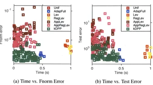
chang-ing across iterations of the Markov Chain. . . . 38 2-6 Time-Error tradeoffs with 50 landmarks on the Ailerons data truncated at

2,000 samples (1,000 training and 1,000 testing). Errors are shown on a log scale. Bottom left is the best (low error, low running time), top right is the w orst. . . . 39

3-1 Lower and upper bounds computed by Gauss-type quadrature in each

itera-tion on uT A-lu with A E RoOxO0. . . . . 57

3-2 Running times (top) and corresponding speedup (bottom) on synthetic data. (k-)DPP is initialized with random subsets of size n/3 and corresponding running times are averaged over 1,000 iterations of the chain. All results are averaged over 3 runs of experiments. . . . 74 4-1 (a) Convergence of marginal and conditional probabilities by DPP on

uni-form matroid, (b,c) comparison between add-delete chain (Algorithm 9) and projection chain (Algorithm 11) for two instances: slowly decaying spectrum and sharp step in the spectrum. . . . . 87 4-2 Results on the CompAct(s) dataset. Results are the median of 10 runs,

except Greedy and Fedorov. Note that Unif, Lev, PL and DVS use less than 1 second to finish experiments. . . . 100 5-1 Convergence of marginal (Ma r g) and conditional (Cond- 1 and Cond-2,

conditioned on 1 and 2 other variables) probabilities of a single variable in a 20-variable Ising model with different (0, 6). Full lines show the means and dotted lines the standard deviations of estimations. . . . 123 5-2 Empirical mixing time analysis when varying dataset sizes, (a) PSRF's for

each set of chains, (b) Approximate mixing time obtained by thresholding PSRF at 1.05. . . . 123 5-3 Convergence of marginal and conditional probabilities by DPP on uniform

m atroid . . . 124 A-1 Relative Frobenius norm and spectral norm error achieved by different

kernel approximation algorithms on the remaining 7 data sets. . . . 128 A-2 Training and test error achieved by different Nystr6m kernel ridge regression

algorithms on the remaining 7 regression datasets. . . . 129 A-3 Performance of Markov chain DPP-Nystr6m with 50 landmarks on Ailerons.

A-4 Performance of Markov chain DPP-Nystr6m with 100 landmarks on Ailerons. Runs for 5,000 iterations. . . . 131 A-5 Performance of Markov chain DPP-Nystr6m with 200 landmarks on Ailerons.

Runs for 5,000 iterations. . . . 132 A-6 Time-Error tradeoff with 20 landmarks on Ailerons of size 4,000. Time and

Errors shown in log-scale. . . . 133 A-7 Time-Error tradeoff with 20 landmarks on California Housing of size 12,000.

Time and Errors shown in log-scale. We didn't include AdapFull, Lev and RegLev due to their inefficiency on larger datasets. . . . 134

B-1 Results on CompAct(s). Note that Unif, Lev, P L and DVS use less than 1 second to finish experiments. . . . 147 B-2 Results on CompAct. Note that Unif, Lev, PL and DVS use less than 1

second to finish experiments. . . . 147 B-3 Results on Abalone. Note that Unif, Lev, PL and DVS use less than 1

second to finish experiments. . . . 147 B-4 Results on Bank32NH. Note that Unif, Lev, PL and DVS use less than 1

second to finish experiments. . . . 148

C-1 Convergence of marginal (Ma rg) and conditional (Cond-1 and Cond-2, conditioned on 1 and 2 other variables) probabilities of a single variable in a 20-variable Ising model. We fix

#

6= 0.5and(c)6 = 0.8.. . . . 157 C-3 Comparisons of PSRF's for marginal estimations with different 6's. (a)

PSRF's with different 6's and (b) the approximate mixing time estimated by thresholding PSRF at 1.05. . . . 158

C-4 Convergence of marginal (Marg) and conditional (Cond-1 and Cond-2, conditioned on 1 and 2 other variables) probabilities of a single variable in a 20-variable Ising model. We fix 6 = 1 and vary

#

#

and (c)

/

/

0 = 2 and (c),3 = 3. . . . 159 C-6 Comparisons of PSRF's for marginal estimations with different O's. (a)

PSRF's with different O's and (b) the approximate mixing time estimated by thresholding of 1.05 on PSRF's. . . . 159 C-7 Convergence of marginal (Marg) and conditional (Cond-1 and Cond-2,

conditioned on 1 and 2 other variables) probabilities of a single variable in a k-DPP on partition matroid base of rank 5, with (a) N = 20; (b) N = 50 and (c) N = 100. Full lines show the means and dotted lines the standard deviations of estimations. . . . 160 C-8 PSRF of marginal (Marg) and conditional (Cond-1 and Cond-2,

condi-tioned on 5 and 10 other variables) probabilities of a single variable in a k-DPP on partition matroid base of rank 5, with (a) N = 20; (b) N = 50 and (c) N = 100. . . . 160 C-9 Convergence of marginal (Marg) and conditional (Cond-5 and Cond-10,

conditioned on 5 and 10 other variables) probabilities of a single variable in a DPP on uniform matroid of rank 30, with (a) N = 50; (b) N = 100 and (c) N = 200. Full lines show the means and dotted lines the standard deviations of estimations. . . . 161 C-10 PSRF of marginal (Marg) and conditional (Cond-5 and Cond-10,

con-ditioned on 5 and 10 other variables) probabilities of a single variable in a DPP on uniform matroid of rank 30, with (a) N = 50; (b) N = 100 and (c) N = 200. . . .. . . .. . .. . . .. .... .. .. ... ... 161

List of Tables

3.1 Data. For all datasets we add an lE-3 times identity matrix to ensure positive definiteness. . . . 75 3.2 Running time and speedup for (k-)DPP. For results on each dataset

(occu-pying two columns), the first column shows the running time (in seconds) and the second column shows the speedup. For each algorithm (occupying two rows), the first row shows results from the original algorithm and the second row shows results from algorithms using our framework. . . . 76

Chapter 1

Introduction

Subset selection problems lie at the heart of many applications where a small subset of items must be selected to represent a larger population. A typical example is kernel matrix approximation [49, 56]. Kernel methods are widely used in machine learning and they need to manipulate kernel matrices with operations like matrix inversion or matrix multiplication. However, the square/cubic time complexity of these operations will be prohibitive when the kernel matrix is large. One solution to large kernel matrix operation is to construct a low-rank approximation of the kernel matrix. Such approximation is done by first selecting a few rows and columns from the kernel matrix. These rows and columns are then multiplied together in certain ways to construct the approximated matrix (See Figure 1-1). Subset selection problems also appear in video summarization [85, 161]. A long video may take tens of hours to watch. To get the main idea of the video quickly, we could create a "trailer" of the video by selecting a subset of scenes and watch the trailer. A similar example is text summarization [119] where we have a large pile of papers to read. Instead of reading the papers page by page, we select a subset of representative paragraphs in the paper and form a summary of all the papers. By reading the summary, we are able understand main ideas in papers within a short time (See Figure 1-1). Another example of subset selection is sensor placement [88, 103]. Here, the task is to monitor a specific area with a certain number of sensors. There are many possible locations to place sensors on. Due to the limited number of sensors, we seek for a subset of locations such that the area monitored by at least one sensor is maximized. (See Figure 1-1).

- - -- Kernel Matrix Approximation

S

-II

Figure 1-1: Applications examples for subset selection: kernel matrix approximation, video/text summarization and sensor placement.

Typically, the selected subsets are expected to fulfill various criteria such as sparsity or diversity. Our focus is on diversity, a criterion that plays a key role in a variety of applications, such as gene network subsampling [19], recommender systems [189], among many others [104, 77, 107, 2, 169, 160].

Diverse subset selection amounts to sampling from the set of all subsets of a ground set according to a measure that places more mass on subsets with qualitatively different items. We call such probability measures Diversity-Inducing Probability Measures (DIPMs). A

well-known example of DIPMs is called Determinantal Point Processes (DPPs). DPPs were first introduced in physics to model the repulsive phenomenon of Fermion particles [127]. Later they were referred to as Determinantal Point Processes [29] and were introduced to machine learning community [107]. Each DPP is associated with a kernel matrix L which quantifies the similarities between items. A DPP captures diversity by assigning subset S probability that is proportional to submatrix determinant (See Figure 1-2). Specifically, we have 7r(S) oc det(Lss).

To illustrate that DPPs capture diversity, we consider sampling a subset of points on a 2-D panel where the dissimilarity between points grows with their distance. We show in

wr(S)

oc

det(Ls,s)

L

&

O

Figure 1-2: DPP definition

Figure 1-3 subsets sampled by DPP versus uniform sampling. If we do uniform sampling where no similarity information between points is considered, we end up with a subset that has clusters at random places. On the other hand, the subset sampled by DPP is spread out,

and each sampled point is far from other points, i.e. the subset is diverse.

DPPs enjoy substantial interest in machine learning [104, 106, 100, 85, 132], in part due to computational tractability of basic tasks such as computing partition functions, sampling, and extracting marginals [94, 107]. Despite being polynomial-time, these tasks remain

1 0.8 0.6 0.4 0.2 0 0 0.5 1 DPP 1 0.8 0.6 0.4 0.2 0 0 0.5 Independent 1

Figure 1-3: Sampled subsets from a 2D panel using DPP and Uniform distribution.

0 0 00 _{o ooo0 o} 0 0 0 0j₀₀ 000 00 00 0~c" 0 0 0 00 a 0 oo oo o0 8 0 0 o * 0 0 000 000 0 non 00 0 o o0 o o o 0 0000 ~% 0 6'a ~ 08 8&' 00 0 0 0 0 6 0 0 0 0

8

infeasible for large datasets. DPP sampling, for example, relies on an eigendecomposition of the DPP kernel, whose cubic complexity is a huge impediment to scalability. Cubic pre-processing costs also impede wider use of the cardinality-constrained variant k-DPP [105]. These drawbacks have triggered work on approximate sampling methods. Much work has been devoted to approximately sampling from a DPP by first approximating its kernel via algorithms such as the Nystrm method [3], Random Kitchen Sinks [153, 1] or matrix ridge approximations [187, 181], and then sample based on this approximation. These methods lead to considerable efficiency gain, but are somewhat inappropriate for sampling because they aim to project the DPP kernel onto a lower dimensional space while minimizing a matrix norm, rather than minimizing an error measure sensitive to determinants. Another approach based on the concept of coresets is proposed to directly minimize the TV distances between the original distribution and the approximated one [112]. This method relies on the structure of the dataset: if the dataset is nicely clustered, the approximation will be both efficient and effective. Alternative approaches use a dual formulation [104], which saves time in preprocessing of the kernel matrix by transforming an eigendecomposition of a large kernel matrix to a smaller one. This is based on the assumption that a low-rank decomposition of kernel matrix is available, which may not always be true.

Another line of work focuses on sampling with Markov chain Monte Carlo [92, 76, 47]. The idea is to maintain an active subset of the ground set, and iteratively update the active set by adding items to or removing items from it. After running certain number of iterations the active subset is viewed as a subset sampled from an approximation of the target distribution. The number of updates needed to produce a good sample from MCMC is low-order polynomial [8, 117]. However, existing Markov chains require storing and updating the inverse of sub-matrices of kernel, which is potentially inefficient. Thus, since its proposal, MCMC sampling from DPP has so far not been used widely in practice.

Nevertheless, DPPs still have huge potential to be applied to subset selection problems where diverse subsets are needed. In the first part of this thesis, we explore the application of DPPs in kernel matrix approximation. We show that with diverse subset of rows and columns selected via DPP, we are able to achieve one of the best performances among existing state-of-art baselines. We further consider applying such approximation to a

downstream application, kernel ridge regression, and show empirically that using DPPs will result in superior performance.

Besides effectiveness, we pursue efficiency in sampling procedure. In the second part of this thesis, we address efficiency of (k-)DPP sampling with MCMC. We accelerate existing MCMC approaches with a retrospective-style algorithmic framework and an ancient technique called Gauss quadrature. Our Markov chain samples valid subsets as existing ones, but is much faster when the kernel L of the (k-)DPP is sparse. In large-scale experiments we observe over 103 times acceleration with our method.

While DPPs are one common example of DIPMs, there is a broader class of probability measures that is diversity-inducing called Strongly Rayleigh (SR) measures. These measures are intimately related to stable polynomials. This viewpoint is first established in [28], which has proved key to uncovering their remarkable properties, both for modeling as well as for fast sampling. SR measures exhibit negative association, a strong, "robust" notion of negative dependence. They have recently emerged as valuable tools in the design of algorithms [6], in the theory of polynomials and combinatorics [28], and in machine learning through DPPs. Despite being important, the mathematical properties of SR measures have largely been unexplored. Only recently in the work of [8] the authors have proved the first poly-time mixing MCMC on a certain class of SR measures called homogeneous SR measures, while the mixing time of MCMC for general SR measuresremains unknown.

For the third part of thesis, we study sampling methods for general SR measures and derive a provably fast mixing Markov chain that is novel and may be of independent interest. Our results provide the first polynomial guarantee for Markov chain sampling from a general DPP, and more generally from an SR distribution. This result also indicates an efficient sampling method for Dual Volume Sampling (DVS), whose poly-time sampling method has remained open since 2013 [13]. Specifically, we prove that DVS lies in the class of SR, thus a poly-time MCMC sampling method follows.

While most DIPMs that we have considered have no explicit constraints, real-world applications usually come with various constraints. Take sensor placement for example. We want to have a precise control over the number of locations sampled, so that we do not end up sampling too many locations (See Figure 1-4). However, little has been known in

*D 0 0

9 0 0

Figure 1-4: In sensor placement problem, we want to control the size of subsets we are sampling so as not to end up with sampling too many locations

efficient sampling methods of constrained DIPMs.

In the last part of this thesis, we study DIPMs with certain constraints. More specifically, we consider matroid base constraints or cardinality constraints. We present theoretical results concerning mixing times of Markov chains for constrained DIPMs, and prove that under certain conditions, all chains mix rapidly. Note that while some of the constrained distributions do lie in the family of SR measures, adding constraints may break the SR property, thus a direct application of fast MCMC for SR measures is not viable, and fast mixing chains have not been known before. We verify empirically that the dependencies of mixing times on several function- or data-related factors are consistent with our analysis.

This thesis is organized as follows: In Chapter 1 we give a brief overview of DIPMs and the problems on which we will focus throughout this thesis. In Chapter 2 we apply DPPs to core machine learning applications including kernel matrix approximation and kernel ridge regressions. We show superior performance of DPP-approximated algorithms. In Chapter 3 we introduce efficient MCMC algorithms for (k-)DPPs accelerated by Gauss-type quadrature. In Chapter 4 we focus on the broader class of SR and show the first poly-time mixing MCMC algorithm. We also revisit Dual Volume Sampling (DVS) and show that DVS lies in the class of SR. In Chapter 5 we consider constrained DIPMs and show efficient MCMC method for these measures. We close this thesis with conclusion and open problems in section 6.

Chapter 2

Determinantal Point Processes for

Kernel Methods

In this chapter, we consider applying DPP to kernel methods, including Nystr6m method and kernel ridge regression. The Nystrm method has long been popular for scaling up kernel methods. However, its theoretical guarantees and empirical performance both critically rely on the selection of suitable landmarks. We study landmark selection via DPPs. We prove that landmarks selected according to a DPP offer guaranteed approximation errors for Nystr6m. Subsequently, we analyze implications for kernel ridge regression, where we also prove the approximation guarantees. For efficient implementation, we use Markov chain DPP accelerated by Gauss quadrature to do the sampling, which will be explained in more details in the next chapter. We present empirical results that support the theoretical analysis, and demonstrate the superior performance of DPP-based landmark selection compared against existing approaches. Materials in this chapter are based on [113].

2.1

Introduction

Matrix low-rank approximation is an important ingredient of modern machine learning methods: many methods rely on operations such as multiplication and inversion of matri-ces. Scaling cubically in the number of data points n, these operations quickly become a bottleneck for large data. In such cases, low-rank approximations promise speedups with a

tolerable loss in accuracy.

A notable example is the Nystr6m method [144, 18], which takes a positive semidefinite matrix L E R n" as input, selects from it a small subset S of columns L.,s, and constructs

the approximation L

= Ls,.. The matrix

L, in its factored form, is then used in

place of L. If the number k = ISI of selected columns is small, then using

L decreases

Since its introduction to the machine learning community, the Nystr6m method has been applied to a wide spectrum of problems, including kernel ICA [15, 162], kernel and spectral methods in computer vision [21, 66], manifold learning [178, 177], regularization [157], and efficient approximate sampling [3]. Recent work [46, 14, 4] has shown risk bounds for Nystr6m applied to various kernel methods.

The most important step of the Nystr6m method is the selection of the column subset S, the so-called landmarks. This choice governs the approximation error and subsequent performance of the approximated learning methods [46]. The most basic strategy is to sample landmarks uniformly at random [184]. More sophisticated non-uniform selection strategies include deterministic greedy schemes [168], incomplete Cholesky decomposition [65, 16], sampling with probabilities proportional to diagonal values [56], to column norms [55], based on leverage scores [79], via K-means [186], and using submatrix determinants [22].

We study landmark selection using Determinantal Point Processes (DPP), discrete probability models that allow tractable sampling of diverse non-independent samples [126, 107]. Our work generalizes the determinantal sampling scheme of [22].1 We refer to our scheme as DPP-Nystr6m, and analyze it from several perspectives.

A key quantity in our analysis is the error of Nystrbm approximation. Suppose c is the target rank; then for selecting k > c landmarks, Nystr6m's error is typically measured using the Frobenius or spectral norm, relative to the best achievable error via rank-c SVD L,; that is, we measure

L - L.,sLts Ls,.HF I - L.,sLs, Ls,112

or

| - L|| FL W L - cJ2

Several authors also use additive instead of relative bounds. However, such bounds are very sensitive to scaling, and become loose even if a single entry of the matrix is large. Thus, we focus on the above relative error bounds.

First, we analyze this approximation error. Previous analysis [22] assumes a cardinality of k = c; we go beyond this limitation and analyze the general case of selecting k > c

columns. Our relative error bounds rely on the properties of characteristic polynomials. Empirically DPP-Nystr6m is seen to obtain approximations superior to other state-of-art methods.

Second, we consider its impact on kernel methods. Specifically, we address the impact of Nystr6m-based kernel approximations on kernel ridge regression. This task has been noted as the main application in [14, 4]. We show risk bounds of DPP-Nystrbm that hold in expectation. Empirically, it achieves the best performance among competing methods.

Third, we consider the efficiency of DPP-Nystr6m; specifically, its tradeoff between error and running time. Since its proposal in [22], determinantal sampling (also realized as k-DPP) has so far not been used widely in practice due to (valid) concerns about its scalability. We use MCMC for DPP sampling and accelerate it with Gauss quadrature. Empirical results indicate that the chain yields favorable results within a small number of iterations, and the best efficiency-accuracy traedoffs compared to state-of-art methods (Figure 2-6).

2.2

Background and Notation

Let L

E

L.j for the j-th column, and, likewise, Ls,. for the rows of L and L.,s for the columns of L indexed by S C [n]. Finally, Ls,s is the submatrix of L with rows and columns indexed by S. In this notation, L, = U.,[,]A[c,,[] UT is the best rank-c approximation to L in both Frobenius and spectral norm. We write r(-) for the rank and (-)t for the pseudoinverse, and denote the decomposition of L by BT B, where B c R( .

|= k landmarks, and approximates L with L.,sL s Ls,.. The actual set of landmarks affects the approximation quality, and has hence been the subject of a substantial body of research [46, 168, 65, 16, 56, 55, 79, 186, 22].

Besides various landmark selection methods, there exist variations to the standard Nystr6m method, such as the ensemble Nystrim method [108] that uses a weighted combi-nation of approximations, or the modified Nystrm method that constructs an approximation L.,sLt sLL,.Ls,. [175]. In this chapter, we focus on the standard Nystr6m method.

2.3 DPP for the Nystro*m Method

Next, we consider sampling landmarks S C [n] from k-DPP(L), and use the approximation Ls = L.,sLtsLs,., referred to as DPP-Nystrbm. This method was introduced in [22], but

without making the explicit connection to DPPs. Our analysis builds on this connection and subsumes existing results which only apply to k = c (recall, c is the rank of the target approximation).

In the remainder of this section, we show following bounds:

Theorem 1 (Relative Error). If S ~ k-DPP(L), then DPP-Nystrbm satisfies the relative errors bounds

| L - L.,s(Ls,s)tLs,.F]

k +

I21

ES JL - Le||F - +1 -c C(.31

ES [HL - L.<s(LsY~LsJJ₂] < k+I (n - c). _(2.3.2)

1 IL - Le|2 -k +1 - c

Our analysis exploits a property of characteristic polynomials observed in [89]. Coeffi-cients of characteristic polynomials are a sum of determinants:

ek(L) = det(BsBs) = ek(A). (2.3.3)

I S1 =k

Lemma 2 ([89]). For any k > c > 0, it holds that

1

k+1( ) <_IE____ ek(A) - k + I1 - c i

With this lemma in hand, we proceed to prove Theorem 1.

Proof (Thm. 1). We begin with the Frobenius norm error, and then show the spectral norm result. Using the decomposition L = BT B, it holds that

ES [H|L - L.,sLt Ls,.HF = [BT [EJ B - BT Bs(BT Bs T B||F]

= Es

[J

where UsEsVs is the SVD of Bs. Next, we extend Us to a full basis U = [Us U.-]. Since

U is orthonormal, we have UUT = I and I - UsUST = USL(U4)T. Plugging in this identity

and applying Cauchy-Schwartz yields

E (I - UsUT)B|F]

=ES

[J|B

V

(b U (U Tbj) I) = 'E~ st ~b U| = ek(L) Is

ek(L) SIs=k

S

= (k + 1) ek+1(L)

ek (L)

By (2.3.3) and Lemma 2 it follows that

(k + 1)ekL < +1A kk (L - C i-c = k /n- c-c --k+l-c ri cHJL - LcHJF. (1: .bTU-LJ l b 11U2) det (BT Bs)J|bTUSI|| A e < ES _I

The bound on the Frobenius norm immediately implies the bound on the spectral norm:

ES

[H|L

L|L

< kn - c||L - L||F < (n - c)||L - Lc12 E

k +I- c k +I- c

Remarks Our bounds are not directly comparable to previous bounds (e.g., [79] on uniform and leverage score sampling) that hold with certain probability since our bounds hold in expectation. However, in Sec. 2.5.1 we extensively experiment with DPP-Nystrbm on various datasets and observe superior accuracies against various existing state-of-art methods.

We also show the bounds that hold with high probability. To show high probability bounds we employ concentration results on homogeneous strongly Rayleigh measures. Specifically, we use the following theorem.

Theorem 3 ([150]). Let P be a k-homogeneous strongly Rayleigh probability measure on

{0, 1}" and

f

P(f - E[f] > af) < exp{-a2_/8k}.

It is known that a k-DPP is a homogeneous strongly Rayleigh measure on {0, 1}' [28, 8], thus Theorem 3 applies to results obtained with k-DPP. Concretely, for the bound in Theorem 1 that holds in expectation, we have the following bound that holds with high probability:

Corollary 4. When sampling S ~ k-DPP(L), for any 6 E (0, 1), with probability at least 1 - 6 we have

IL - L.,s(Ls,s)tLs,.|F

+

/n -c + Z8k log (1/X6) _{2 ,7_=}

|IL - LC||F k+1 -c Z=c+1 I

IL - L.,s(Ls,s)tLs,.|2 _{k + (N - c) + -/8k log(/6)A}

Proof The Lipschitz constants of the relative errors are upper bounded by and

AI respectively. Applying Theorem 3 yields the results.

2.4 Low-rank Kernel Ridge Regression

The theoretical (Section 2.3) and empirical (Section 2.5.1) results suggest that DPP-Nystrbm may be very suitable for scaling kernel learning methods. In this section, we analyze its implications on kernel ridge regression. The experiments in Section 2.5 confirm our results empirically.

Suppose we have n training samples {(X,, y,)}I1, where yj = zi + ci are the observed labels under zero-mean noise, with finite noise covariance. We minimize a regularized empirical loss

min

-

fcF n2

over an RKHS F; equivalently, we solve the problem

min _{f(yi, (L)j) + a Loz,}

aERn)

2

for the corresponding kernel matrix L. With the squared loss f(y, f(x)) =(y - (X))2, the resulting estimator is

n

f(x) Zai k(x, xi), a = (L + nyI) -y, (2.4.1)

covariance by F, we obtain the risk

R{s) = Ez- z|2

n

= ny2_{ZT(L + nyI)-}2_{z + !Tr(FL}2_{(L + n--I)-}2₎

= bias(L) + var(L). (2.4.2)

Observe that the bias term is decreasing (in L) while the variance term is matrix-increasing. Since the estimator (2.4.1) requires expensive matrix inversions, it is common to replace L in (2.4.1) by an approximation L. If L is constructed via Nystrdm we have Li -< L, and it directly follows that the variance shrinks with this substitution, while the bias

increases. Denoting the predictions from

L by L, Theorem 5 completes the picture of how

i

Theorem 5. If L is constructed via DPP-Nystrom and - ;> Tr( L), then

ES > I - (k + 1) ek+1(L)

IZR( ) ny ek(L)

Proof We build upon [14]. Knowing that Var(L) < Var(L) as

Ii

the bias. We write L BT B and L - BTB(BT Bs)tBT B, and bound the difference L - L as

L - = BT(I - Bs(BT Bs)tBT)B = BT US(USF)T B

B BT _{UA (U )}T _{B =F E (bTUg(US )Tb}

3)2I

i'j

S/( |b UI||22 ||bT UI2)1 =

E

V2,J

where

vs

E Ir

(b

<

,

E j7

-LTr(L)

-Y,

have that L < 1, and

(L + nmyI)-<- (L - vsI + nyI)-1 (1 - )-(L +

nI)-

_.

Finally, this matrix inequality imples that

bias(L) ( s

bias(L) nry

Taking expectation over S - k-DPP(L) yields

ES bias(L) > 1-ES VS 1 (k + 1) ek+1 (L)

bias(L) [nyj nY ek(L)

Together with the fact that var(L) > var(L), we obtain

[_(_)

_ZiAj

for any k > c, where the last inequality follows from Lemma 2 and - ;> ITr(L). E

Remarks. Theorem 5 quantifies how the learning results rely on the decay of the spectrum of L. In particular, the ratio ek+1(L)/ek(L) closely relates to the effective rank of L: if Ak > a and Ak+1 < a, this ratio becomes almost zero, resulting in near-perfect approximations and no loss in learning. This also becomes evident in (2.4.4).

Again for the bound in Theorem 5 that holds in expectation, we have the following bound that holds with high probability:

Corollary 6. If i is constructed via DPP-Nystr5m, then with probability at least 1 -bias(L)

is upper-bounded by

1 + 1 ((k+1)ek+l(L) + N/8k log(1/)tr(L)).

n-y e ( L)

Proof Consider the function fs(L) = vs = Ji IIb7 (US)-L I Ej | = tr(L). Since 0 < fs(L) < tr(L), it follows that the Lipschitz constant for fs is at most tr(L). Thus

when S ~ k-DPP and 6 E (0, 1), by applying Theorem 3 we see that the inequality

vs E [vs] + 8k log(1/)tr(L) holds with probability at least 1 - 6. Hence

bias(L) ils ]t+V(L)

-ES < I + E + klog(1/)tr(L)

bias((L) ny ny

= +-y- (k ()ek + V8k log(1/6)tr(L)

holds with probability at least 1 - 6.

There exist works considering DPP methods in this scenario [14, 4]. Although our bounds are not directly comparable to existing ones, we do extensive experiments to com-pare DPP-Nystr6m against other state-of-art methods in Sec. 2.5.2 and observe superior performance of DPP-Nystr6m.

2.5

Experiments

In our experiments, we evaluate the performance of DPP-Nystr6m on both kernel approxi-mation and kernel learning tasks, in terms of running time and accuracy.

We use 8 datasets: Abalone, Ailerons, Elevators, CompAct, CompAct(s), Bank32NH, Bank8FM and California Housing2. We truncated each dataset to be 4,000 samples (3,000 training and 1,000 testing). Throughout our experiments we use an RBF kernel and choose the bandwidth parameter o and regularization parameter A for each dataset by 10-fold cross-validation. We initialize the Gibbs sampler via Kmeans++ and run for 3,000 iterations.

Results are averaged over 3 random subsets of data.

2.5.1

Kernel Approximation

We first explore DPP-Nystr6m (kDPP in the figures) for approximating kernel matrices. We compare to uniform sampling (Un i f) and leverage score sampling (Lev) [79] as baseline landmark selection methods. We also include AdapFull (AdapFu 11) [50] that performs

2

The data is available at http://www.dcc.fc.up.pt/~ltorgo/Regression/DataSets. html

-. Unif . .AdapFull -.. Lev 0.06 0.06 RegLev S....kDPP

@

Figure 2-1: Relative Frobenius/Spectral norm errors from different kernel approximation algorithms on Ailerons dataset.

quite well in practice but scales poorly, as 0(n2), with the size of dataset. Although sampling with regularized leverage score (RegLev) [4] is not originally designed for kernel approximation, we include its results to see how regularization affects leverage score sampling.

Figure 2-1 shows example results on the Ailerons data. DPP-Nystrom performs well, achieving the lowest error as measured in both spectral and Frobenius norm. The only method that is on par in terms of accuracy is AdapFull, which has a much higher running time.

For a different view, Figure 2-2 shows the improvement in error over Un if. Relative improvements are averaged over all data sets. Again, the performance of DPP-Nystrbm almost always dominate those of other methods, and achieves an up to 80% reduction in error.

2.5.2

Kernel Ridge Regression

Next, we apply DPP-Nystr6m to kernel ridge regression, comparing against uniform sam-pling (Unif) [14] and regularized leverage score samsam-pling (RegLev) [4] which have theoretical guarantees for this task. Figure 2-3 illustrates an example result: non-uniform sampling greatly improves accuracy, with kDPP improving over regularized leverage scores

- Spec Error , . Fro Error

Fro Imprpvement 80 - - 80 -E E ) 70- 70-0o ₀ C0L -9 60- 60--- AdapFull S 50 -- 50 Lev RegLev CC_..-.. _kDPP 20 40 60 80 100 20 40 60 80 100 # landmarks # landmarks

Figure 2-2: Improvement in relative Frobenius/spectral norm errors (%) over Uni f (with corresponding landmark sizes) for kernel approximation, averaged over all datasets.

in particular for a small number of landmarks, where a single column has a larger effect. Figure 2-4 displays the average improvement over Unif, averaged over 8 data sets. Again the performance of kDPP dominates those of RegLev and Unif and leads to gains

in accuracy. On average kDPP consistently achieve more than 20% improvement over

Unif.

2.5.3

Mixing of the Markov Chain DPP

In the next experiment, we empirically study the mixing of the Markov chain with respect to matrix approximation errors, the ultimate measure that is of interest in our application of the sampler. We use k = _{50 and vary n from 500 to 4,000. To exclude impacts of the}

initialization, we pick the initial state So uniformly at random. We run the chain for 5,000 iterations, monitoring how the error changes with the number of iterations. The example results in Figure 2-5 show that empirically, the error drops very quickly and afterwards fluctuates only little, indicating a fast convergence of the approximation error. Further results

may be found in the supplementary material.

Notably, our empirical results suggest that the mixing time does not increase much even if n increases greatly, suggesting that the MCMC sampler remains fast even for large n

0 a) 30 25 20 15 10 5 0

Train Error Test Error

30 25 -20 -2 15- 10-5 0 20 40 60 80 100 20 40 60 80 100 # landmarks # landmarks

Figure 2-3: Training and testing errors by different Nystrom-approximated kernel ridge regression algorithms on Ailerons dataset.

Train Improvement 60 - 35o-U) E - U40-0 E E30 - 20-20 40 60 80 100 # landmarks 10 -I-20 Test Improvement RegLev - kDPP \4000-40 60 80 100 # landmarks

Figure 2-4: Improvements in training/testing errors (%) over uniform sampling (with corresponding landmark sizes) in kernel ridge regression, averaged over all datasets.

37 -- Unif RegLev -kDPP 60- ,50-C a) E 40 -0 U_ E 30 - 20-76 10

.1-

I

0.02 0.015 -0.01 -0.005 0 Size=1000 Size=500

r

Figure 2-5: Relative Frobenius norm error of DPP-Nystr6m with 50 landmarks as changing across iterations of the Markov Chain.

0 U) 0.02-0.015 = 0 0 C LL 0.005--L 0 0.01

LUM40*444

2.5.4

Time-Error Tradeoffs

(a) Time vs. Fnorm Error (b) Time vs. Test Error

Figure 2-6: Time-Error tradeoffs with 50 landmarks on the Ailerons data truncated at 2,000 samples (1,000 training and 1,000 testing). Errors are shown on a log scale. Bottom left is the best (low error, low running time), top right is the worst.

Iterative methods like the MCMC sampler offer tradeoffs between time and error. The longer the Markov Chain runs, the closer the sampling distribution is to the desired DPP, and the higher the accuracy obtained by Nystr6m. We hence explicitly show the time and accuracy for 0 to 300 iterations of the sampler.

A similar tradeoff occurs with leverage scores. For the experiments in the other sections, we computed the (regularized) leverage scores for Lev and RegLev exactly. This requires a full, computationally expensive eigendecomposition. For a fast, rougher approximation, we here compare to an approximation mentioned in [4]. Concretely, we sample p elements with probability proportional to the diagonal entries of kernel matrices Lij, and then use a Nystr6m-like method to construct an approximate low-rank decomposition of L, and compute scores based on this approximation. We vary p from 50 to 500 to show the tradeoff for approximated leverage score sampling (AppLev) and regularized leverage score sampling (AppRegLev).

Figure 2-6 summarizes and compares the tradeoffs offered by these different methods. The x-axis indicates time, the y-axis error, so the lower left is the preferred corner. We see that exact leverage scores are accurate but expensive, whereas the approximate versions

empirically lose accuracy. AdapFu 11 is accurate but needs longer time than kDPP. These results are sharpened as n grows. Overall, DPP-Nystr6m offers the best tradeoff of accuracy versus efficiency.

2.6 Summary

In this chapter, we explore the use of k-DPP for sampling good landmarks for the Nys-tr6m method and its further application to kernel ridge regression. We theoretically and empirically observe its competitive performance, for both matrix approximation and ridge regression, compared to state-of-the-art methods. To make this accurate method scalable to large matrices, we consider sampling via MCMC accelerated with Gauss quadrature. Our results indicate that the iterative approach, an MCMC sampler, achieves good landmark samples quickly. Our empirical results demonstrate that among state of the art methods, the iterative sampler yields the best tradeoff between efficiency and accuracy.

Chapter 3

Sampling DPP by Efficient MCMC with

Gauss Quadrature

In this chapter, we focus on Markov chain Monte Carlo sampling for (k-)DPP. We show that the chain involves heavy computation of bilinear inverseforms (BIFs) uTA--u, where A is a positive definite matrix and u a given vector. To accelerate the chain, we present a framework for accelerating a spectrum of machine learning algorithms that rely on computation of BIFs. Our framework is built on Gauss-type quadrature and can easily scale to large, sparse matrices; it allows retrospective computation of lower and upper bounds on uT A--u, which in turn helps accelerate several algorithms. We prove that these bounds improve iteratively, compare their tightness to each other, and show their linear convergence. To our knowledge, our work is the first to demonstrate these key properties of Gauss-type quadrature, which is a classical and exceptionally well-studied topic. We illustrate empirical consequences of our results by using quadrature to accelerate Markov chain (k-)DPP and observe tremendous speedups in several instances. Materials in this chapter are based on [118].

3.1

Bilinear Inverse Forms (BIFs)

Symmetric positive definite matrices abound in machine learning, arising in various guises: covariances, kernels, graph Laplacians, or otherwise. A basic computation with such matrices is the evaluation of the bilinear form uTf(A)v, where

f

v are given vectors. If f(A) = A- 1, we speak of computing the bilinear inverseform (BIF) uTA-lv. If, for instance, u=v=ei (1th canonical vector), then uTf(A)v = (A--1)i is the ith

diagonal entry of the inverse.

In this chapter, we are specifically interested in computing BIFs due to their great value in several machine learning contexts, including the evaluation of a Gaussian density at a point, the Woodbury matrix inversion lemma, implementation of MCMC samplers for Determinantal Point Processes (DPP), computation of graph centrality measures, or greedy

submodular maximization (see Sec. 3.1.3).

When A is large, it is preferable to compute u TAlv iteratively rather than first com-puting A-'v (using Cholesky) at a cost of 0(n3) operations. One idea is to use conjugate gradients to approximately solve Ax = v and to then obtain u TA-v = UTTx. But several applications require precise bounds on numerical estimates to uTA-lv (e.g., in MCMC based DPP samplers such bounds help decide whether to accept or reject a transition in each iteration-see Sec. 3.6.1), so we need a more finessed approach.

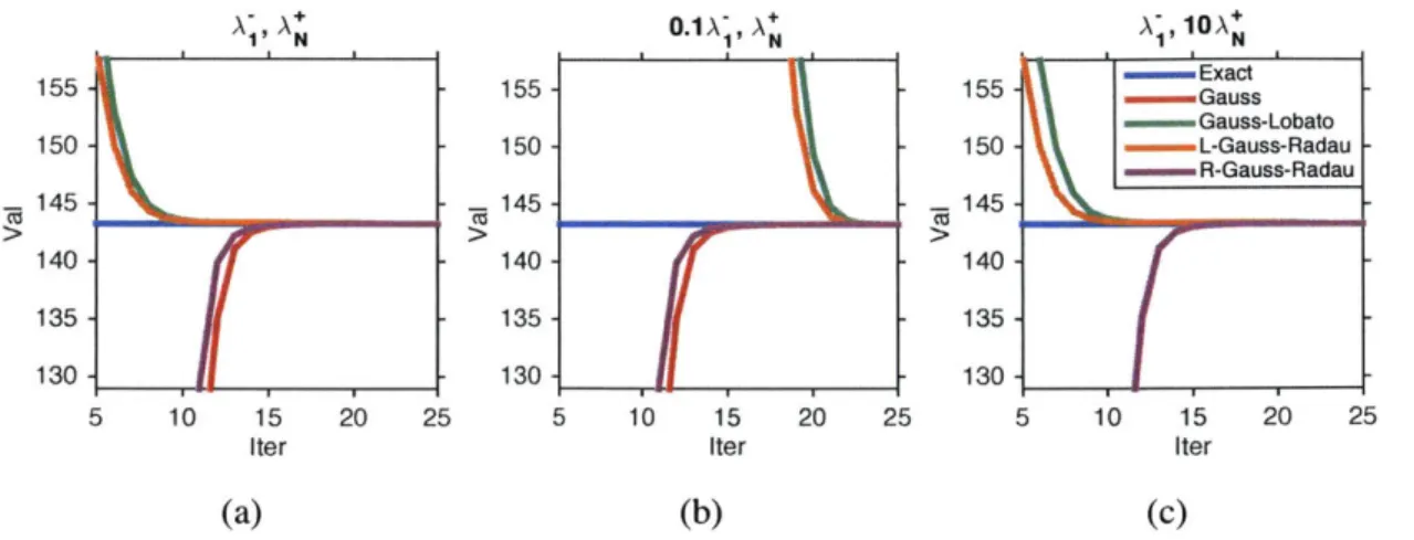
Gauss quadrature is such an approach. Originally proposed in [71] for approximating integrals, Gauss- and Gauss-type quadrature (i.e., Gauss-Lobatto [122] and Gauss-Radau [152] quadrature) have since been applied to approximating bilinear forms including the BIF uT A-lv [17]. [17] also show that Gauss and (right) Gauss-Radau quadrature yield lower bounds, while Gauss-Lobatto and (left) Gauss-Radau yield upper bounds on this bilinear inverse form.

Despite its long history and voluminous existing work (see e.g., [82]), our understanding of Gauss-type quadrature for matrix problems is far from complete. For instance, it is not known whether the bounds on BIFs iteratively improve; nor is it known how the bounds obtained from Gauss, Gauss-Radau and Gauss-Lobatto quadrature compare with each other. We do not even know how fast the iterates of Gauss-Radau or Gauss-Lobatto quadrature converge to the true value of uTA-lV.

Contributions. We address all the aforementioned problems, and make the following main contributions:

- We show that the lower and upper bounds generated by Gauss-type quadrature monoton-ically approach the target value (Thm. 12, Thm. 14, Corr. 15). Furthermore, we show