Boost through reentry trajectory planning for maneuvering reentry vehicles

(1)

Boost Through Reentry Trajectory Planning For

Maneuvering Reentry Vehicles

by

Matthew James Abrahamson

S.B., Aerospace Engineering With Information Technology Massachusetts Institute of Technology (2006)

Submitted to the Department of Aeronautics and Astronautics in partial fulfillment of the requirements for the degree of

Master of Science in Aeronautics and Astronautics at the

MASSACHUSETTS INSTITUTE OF TECHNOLOGY May 2008 MASSACHUSETTS INSTrITTE. OF TECHNOLOGY

OCT

13 2009

LIBRARIES

P/>

Certified by: Accepted by: xRonald J. Proulx, Ph.D.

Principal Member of the Technical Staff The Charles Stark Draper Laboratory, Inc. Technical Supervisor

SJohn

Deyst, Ph.D. Professor of Aeronautics and Astronautics ThesisAdvisor

D v L. Darmofal, Ph.D. Asso jite Department Head Chair, Committee on Graduate Students ~

(2)

(3)

Boost Through Reentry Trajectory Planning For Maneuvering

Reentry Vehicles

by

Matthew James Abrahamson

Submitted to the Department of Aeronautics and Astronautics on May 23, 2008, in partial fulfillment of the

requirements for the degree of

Master of Science in Aeronautics and Astronautics

Abstract

New trajectory planning concepts are explored for rapidly planning a long range, boost-through-reentry mission, using a lightweight, highly maneuverable reentry vehicle. An Aimpoint Map, a set of all possible piercepoints through which a boost-through-reentry trajectory can be flown to a fixed target, contains valuable information about the joint capabilities of the booster and the reentry vehicle. At each piercepoint in the Aimpoint Map, a set of velocities and flight path angles exist that can be reached from launch as well as a set of velocities and flight path angles that allow the target to be reached from the piercepoint. The intersection of these velocity and flight path angle sets provides important information for the trajectory planner about the margins available at each piercepoint in the Aimpoint Map. Boost-through-reentry trajectory optimization is used with a six degrees-of-freedom (6DOF) vehicle model to provide a quantitative assessment of the limiting capabilities of the vehicle flight subject to complex terminal and path constraints. Particular constraints of interest include energy management, max g's, heat-ing rate, final velocity and flight path angle, angle of attack, over-flight considerations, approach azimuth, and booster stage disposal.

Technical Supervisor: Ronald J. Proulx, Ph.D. Title: Principal Member of the Technical Staff

Thesis Advisor: John Deyst, Ph.D.

(4)

(5)

Acknowledgments

First and foremost, I would like to thank Draper Laboratory for the funding and oppor-tunity to perform interesting research over the past two years. Also, I would like to thank my advisor, Ron Proulx, for his ideas and insights that have helped me through the thesis process. Many thanks to Stan Shepperd for providing lectures on everything from Kalman filtering to politics and also serving as a great mentor and friend. Many thanks also to Lee Norris for teaching me how to really put a good powerpoint presentation together. Also thanks to Professor John Deyst for his thoughtful comments on my thesis work as well as his guidance in 16.62x and 16.06.

As I recall the six years I have spent at MIT, there are two things that stand out in my mind as invaluable experiences: Phi Delta Theta Fraternity and The MIT Festival Jazz Ensemble. Some of my most rewarding experiences have come as a member of Phi Delta Theta. It was truly the one experience that made me feel "at home" at MIT. Learning to live and self-govern a house of 40 men is no easy task, and I believe that this experience builds great character and leadership qualities in a young man. I strongly believe in the values and vision of the Fraternity: friendship, sound learning, and moral rectitude. I also take the fraternity motto "One Man Is No Man" to hold true since my journey through MIT would not have been possible without the help and society of others. I only hope that more Fraternities around the country abandon the stereotypical "animal house" culture and return to the core values of Greek life. My experiences in the MIT Festival Jazz Ensemble (FJE) have also given me many rewarding experiences. I would like to thank my director, Dr. Fred Harris, for his creative and humorous instruction during Tuesday and Thursday night rehearsals. They provided a necessary "mind-relief' from the engineering number crunching performed during the day. I would also like to thank Fred for his dedicated effort to make each and every FJE concert a memorable one. I've played alongside jazz greats such as Kenny Werner, Steve Turre, Joe Lovano, Jeff Galindo, Greg Hopkins, and many more due to his hard work.

I would like to thank the AIMSense team for a great run through the Lunar Ventures Business Plan Competition and the MIT 1K Competition. I hope to collaborate with you

(6)

on more entrepreneurial activities in the future.

Finally, I'd like to thank my family and my girlfriend, Shannon, for their love and support over the past few months. I've had to make some sacrifices to complete this thesis and it wouldn't have been possible without their help and support.

This thesis was prepared at The Charles Stark Draper Laboratory, Inc., under Project 22203-004,, Trajectory Optimization, Contract CON01759-7.

Publication of this thesis does not constitute approval by Draper or the sponsoring agency of the findings or conclusions contained herein. It is published for the exchange and stim-ulation of ideas.

3Matthew

J. Abralmson

Date

(7)

(8)

[This page intentionally left blank.]

(9)

4.2.1 Optimality Conditions . . . .. 4.3 Knotting Conditions ... . ... ... 4.4 Parameter Scaling... .. . . . ... 4.4.1 Scaling M ethod ... ... 4.4.2 Segmented Scaling . ... . . . . . . . . .. 4.5 Summary ... .... .... ... 5 The 5.1 Boost Problem Launch Vehicle 5.1.1 Mass Sizing ...

5.1.2 Propellant Burn Rates .. 5.1.3 Thrust Force ... 5.1.4 Booster Length ... 5.1.5 Summary ... 5.2 Environment Models ... 5.2.1 Ellipsoidal-Earth Model 5.2.2 Atmosphere Model . ... 5.3 Launch Vehicle Aerodynamics . . 5.4 Launch Vehicle Attitude Control

5.4.1 Thrust Vector Control . . 5.4.2 Attitude Control System .

. . . . .. .. . . .. . . . .. 114 . . . . . .. . . . . . .. 119 . . . . . . . . . .. 120 . . . . . . . . .121 . . . ... . . . . 123 . . . . . . . . . . . . .. 123 . . . .123 . . . . . . . . . . .125 . . . . . . . . . 12 7 . . . .136 .. . . . . . . . . . .136 . . . .138 84 89 90 90 91 93 94 96 97 98 101 104 105 110 111 113 113

(11)

5.4.3 Aerodynamic Torques . . . ... 5.4.4 Launch Vehicle Control Summary . . . 5.5 Launch Optimal Control Problem Formulation

5.5.1 Initial Conditions ... 5.5.2 Knots . ... 5.5.3 State Bounds ... 5.5.4 Control Bounds ... 5.5.5 Event Constraints . ... 5.5.6 Path Constraints ... 5.6 Launch Vehicle Capabilities . ...

5.6.1 Initial Guess ...

5.6.2 Maximum Piercepoint Range Case . . 5.7 Minimum Piercepoint Range Case . . . . 5.8 Summary . . ...

6 The 6.1

Reentry Problem

Reentry Vehicle Aerodynamics 6.2 Reentry Vehicle Control

6.3 Problem Formulation . . . ... 6.3.1 The Submunitions Deployment 6.3.2 Knots . ...

6.3.3 State Bounds . . . ... 6.3.4 Control Bounds . . . .. 6.3.5 Event Constraints . . . . 6.3.6 Path Constraints . . . . 6.4 Reentry Vehicle Capabilities . . . . . 6.4.1 Ballistic Reentry . . . . 6.4.2 6.4.3 . . . . . . . . . . . . . 167 Missio Maximum And Minimum Downrange Maximum Crossrange ... 6.5 Summary ... 11 . . . . 169 ... 169 n . . .. . . . . . . . 169 . . . .. 171 . . . . . . . 172 . . . . . . . 173 . . . . . . .173 . . . . . . . 174 . . . . . . . 176 . . . . . . .177 . . . . . . . 180 . . . . . . 186 . . . .. 188 138 140 140 140 141 143 144 144 145 147 147 153 158 162 163 164

(12)

7 The Aimpoint Map 191

7.1 Aimpoint Boundaries ... 192

7.1.1 Corner Point Case ... 192

7.2 Aimpoint Minimum and Maximum Piercepoint Cases ... 204

7.3 Launch Footprint ... ... 211

7.3.1 Launch Footprint Trends ... ... 217

7.4 Reverse Reentry Footprint ... ... 220

7.4.1 Reverse Footprint Trends ... ... 222

7.5 Piercepoint V-Gamma Map ... 229

7.5.1 Minimum Point Case ... ... 230

7.5.2 Corner Point Case ... . ... 231

7.5.3 Maximum Point Case ... ... 232

7.5.4 Interior Point Cases ... . ... 233

7.6 Summary ... .... ... 236

8 Conclusions 237 8.1 Future Work ... ... 239

(13)

List of Figures

1-1 Conceptual Vehicle Body With L/D - 2 . ... 1-2 Relationship Between Attitude And Lift In The Lift Plane ...

1-3 Relationship Between Lift And Attitude As Observed By Looking Along The Velocity Vector Direction ...

1-4 Depiction Of A Bank-To-Turn Vehicle, As Seen From Behind The Vehicle Tail ...

1-5 Depiction Of Potential Trajectory Planning Concepts For The New Rapid, Long Range Mission ...

2-1 Earth Centered Inertial Coordinate Frame ... 2-2 Earth Centered Earth Fixed (ECEF) Frame . ... 2-3 Reference (REF) Coordinate Frame . ... 2-4 Up-Downrange-Crossrange Coordinate Frame ... 2-5 Velocity Frame ...

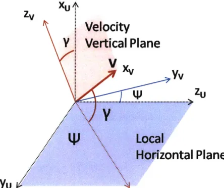
2-6 Representation of Velocity Vertical Frame and Local Horizontal Frame . 2-7 Body Coordinate Frame . . . ...

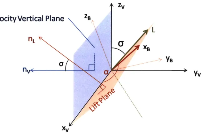
2-8 Relationship Between Sigma and Alpha . ... 2-9 Illustration Of The Lift Plane . ... 2-10 Relationship Between Sigma And The Lift Vector ...

3-1 Position And Velocity States Of The 6DOF System ... 3-2 Illustration Of Relationship Between Frame A And Frame B .

4-1 Example of Knot Locations Along Vehicle Trajectory . . . .

. . . . . . 54

(14)

4-2 Scaled States Using Scaling Method ... ... 108

4-3 Scaled Rates Using Scaling Method ... . 109

4-4 Scaled States Using Segmented Scaling ... ... . . . . . 111

5-1 Flight Segments Of The Boost Portion Of Flight . ... 114

5-2 Illustration of Launch Vehicle Parameters . ... 116

5-3 Isp Variation Over Altitude ... ... ... 121

5-4 Oblate Earth Model With Geodetic Altitude, h, and Geodetic Latitude, K 124 5-5 Comparison Of Atmospheric Density Models Versus Altitude ... 126

5-6 Algorithm Sequence For Automatic Density Curve Fit . ... 127

5-7 Axial Coefficient Of Force As A Function Of Mach Number And Angle Of Attack ... .... ... ... .130

5-8 Normal Coefficient Of Force As A Function Of Mach Number And Angle Of Attack ... ... 131

5-9 The Normalized Center Of Pressure As A Function Of Angle Of Attack And Mach Number ... ... 132

5-10 The Angle of Attack-Averaged Curve Fit To The Axial Coefficient Of Force Plotted Versus Mach Number ... ... 134

5-11 The Mach Number-Averaged Curve Fit For Normal Coefficient Of Force Plotted Versus Angle Of Attack ... 134

5-12 The Angle of Attack-Averaged Curve Fit For Center Of Pressure Plotted Versus Mach Number ... ... 135

5-13 In Plane and Out of Plane Thrust Vectoring Control . ... 137

5-14 External Aerodynamic Torque ... ... ... 139

5-15 Knot Locations Along Launch Trajectory .. ... 142

5-16 Altitude Versus Relative Longitude For Guess Trajectory . ... 148

5-17 Earth-Relative Velocity Versus Time For Guess Trajectory . ... 149

5-18 Flight Path Angle Versus Time For The Guess Trajectory . ... 149

5-19 Nose Pitch Angle Profile For Guess Trajectory . ... 150 5-20 Dynamic Pressure As A Function Of Altitude For The Guess Trajectory . 151

(15)

5-21 5-22 5-23 5-24 5-25 5-26 5-27 5-28 5-29 5-30

Body Pitch Rate Versus Time For Guess Trajectory . ... 152

Maximum Range Boost Trajectory ... . . . 153

Flight Path Angle Profile For Maximum Range Launch Trajectory ... 155

Nose Pitch Angle Profile For Maximum Range Launch Trajectory ... 155

Body Pitch Rate Profile For Maximum Range Trajectory ... . 156

Pitch Controls For Maximum Range Launch Trajectory ... 157

Minimum Range Launch Trajectory ... ... 159

Flight Path Angle Profile For Minimum Range Launch Trajectory ... 159

Nose Pitch Angle Profile For Minimum Range Launch Trajectory ... 160

Drag Profile For Minimum Range Launch Trajectory . ... 161

6-1 Reentry Flight Profile ... ... 164

6-2 Reentry CN as a Function of Angle of Attack . ... 165

6-3 Reentry Vehicle Cx as a Function of Mach Number (M) . ... 166

6-4 Reentry Vehicle Control Flaps ... ... 167

6-5 Submunitions Profile In Terms Of Relative Longitude And Relative Latitude170 6-6 Knots Locations For The Reentry Problem . ... 171

6-7 Ballistic Reentry Trajectory ... ... ... . . 177

6-8 Nose Pitch Angle Profile For Ballistic Reentry Trajectory ... . 178

6-9 Velocity And Flight Path Angle Profiles For The Ballistic Reentry Trajectory179 6-10 Comparison Of Maximum And Minimum Downrange Reentry Trajectories 181 6-11 Velocity And Flight Path Angle Profiles For Minimum Range Reentry Tra-jectory ... ... 182

6-12 Velocity And Flight Path Angle Profiles For Maximum Range Reentry Trajectory ... ... ... 183

6-13 Nose Pitch Angle Profile Versus Time For Minimum Range Reentry Tra-jectory ... ... ... 184

6-14 Nose Pitch Angle Profile For Maximum Range Reentry Trajectory ... 184 6-15 Optimal Pitch Flap Control For The Minimum Range Reentry Trajectory . 185 6-16 Optimal Pitch Flap Control For The Maximum Range Reentry Trajectory 185

(16)

Maximum Crossrange Reentry Trajectory . ... 186

Pitch And Yaw Flap Controls For Maximum Crossrange Reentry Trajectory 187 Heading Angle Profile For Maximum Crossrange Trajectory . ... 188

7-1 Illustration Of Geometry Used To Computed Corner Point Trajectory 193 Corner Point Trajectory of Aimpoint Map . . . . Top-View of Corner Point Trajectory . . . . Side-View of Corner Point Trajectory ... Velocity Profile Of Corner Point Trajectory . . . . Flight Path Angle Profile For Corner Point Trajectory Heading Angle Profile For Corner Point Trajectory . . Nose Attitude Profile For Corner Point Trajectory . . . Pitch Control Profile For Corner Point Trajectory . . . Yaw Control Profile For Corner Point Trajectory. . . . . . . . . . 194 . . . . . 195 ... 196 . . . 197 . . . . .198 . . . . .200 . . . 202 . . . . .203 . . . . . 204 7-11 Concept For Sweeping Across The Aimpoint Map To Compute Minimum

And Maximum Boundaries . ... . . . . . . . . . .. 7-12 The Aimpoint Map For The Submunitions Mission . . . . 7-13 Top-View Of Minimum Boundary Trajectories . . . . 7-14 Aimpoint Minimum Boundary Trajectories . . . . 7-15 Flight Path Angle Profile For Minimum Aimpoint Boundary Trajectories . 7-16 Top View Of Maximum Piercepoint Range Trajectories . . . . 7-17 Maximum Boundary Trajectories ...

7-18 Illustration of Skip Regions Along Aimpoint Boundaries . . . . 7-19 Flight Path Angle Profile For Minimum y Trajectory With /Ppierce = 15

deg, Apierce = 4 deg .. .. .. .. .. . .. . . . . . .... 7-20 Flight Path Angle For Shallowest Launch Trajectory For [tpierce = 15 deg,

Apierce - 4 deg . . .. . . . . . . . ... . . ...

7-21 Steepest And Shallowest Launch Trajectories For 1Ipierce = 15 deg, A ierce

= 4 deg ... ... . ...

7-22 Launch Foorprint For [pierce = 15 deg, Apierce = 4 deg . . . . 6-17 6-18 6-19 7-2 7-3 7-4 7-5 7-6 7-7 7-8 7-9 7-10 205 206 207 208 208 210 211 212 213 214 215 216 -- -'~i~-~i- ~r-r;;;;ix-i~-~-in---il-;-i -^ -i- u~- i;~~-~.-rr-e-~-l;;~i --- li- ; ;; ,---~II--,---~- -i-;- i -l--r tl r- ir;i--c--;;;;r-ii-*;-~m-;;rx ~.-n~

(17)

7-23 Maximum And Minimum Velocity Trajectories For pfpierce = 15 deg, Apierce

= 4 deg, ypierce = -31.9 deg ... ... 218 7-24 Piercepoint Locations At Various Ranges For 0 (to) = 4 deg . ... 219 7-25 Launch Footprints For Various Piercepoints Within The Aimpoint Map . . 219 7-26 Piercepoint Located In The Aimpoint Map At p = 15 deg, A = 4 deg . . . 221 7-27 The Reverse Footprint For tpierce = 15 deg, Apierce = 4 deg ... . 221 7-28 Interior Piercepoints Chosen For Comparison Of Reverse Footprints . . . . 223 7-29 Reverse Footprints For Interior Piercepoints . ... 223 7-30 Shallow Reentry Trajectory From ppierce = 19 deg, Apierce = 0 deg ... 224 7-31 Piercepoints Located Along The Maximum Aimpoint Boundary ... 225 7-32 Reverse Footprints For Piercepoints Along The Maximum Aimpoint

Bound-ary ... ... ... 226

7-33 Reverse Footprints For Trajectories With 09 (to) = 4 deg . ... 228 7-34 Piercepoint V-7y Map For Minimum Aimpoint Boundary Piercepoint

Cor-responding To O(to) = 4 deg ... ... 230 7-35 The Piercepoint V-y Map For The Corner Point Trajectory ... 231 7-36 Piercepoint V-7 Map For Maximum Aimpoint Boundary Corresponding

To ip(to) = 26 deg ... ... ... 232 7-37 Piercepoint V-7 Map For ftpierce = 15 deg, Apierce = 4 deg ... 234

(18)

(19)

List of Tables

5.1 Launch Vehicle Properties ... ... 123 5.2 The Axial Force Coefficient Cx As A Function Of Angle Of Attack And

Mach Number ... ... 130

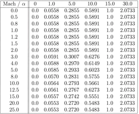
5.3 The Normal Force Coefficient CN As A Function Of Angle Of Attack And

Mach Number ... ... 131

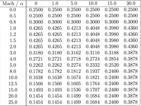
5.4 The Center Of Pressure Cp As A Function Of Angle Of Attack And Mach Number Expressed As A Percentage Of Vehicle Length . ... 132

(20)

(21)

Chapter 1 Introduction

In the years following the end of the Cold War, the United States has seen a dramatic shift in the character of its global adversaries. The state of the world today finds a proliferation of dangerous weapon technologies to small, decentralized extremist groups operating in some of the most remote locations of the world. As these threats continually evolve, so must our preparedness. While the U.S. nuclear arsenal has proved valuable in the past for satisfying the nation's deterrence policies against other superpower nations such as the USSR and China, it provides no such deterrence against emerging rogue threats. A rapid, long range, conventional weapon capability is desired to counter such emerging threats.

Current rapid, long range vehicle capabilities include Intercontinental Ballistic Missiles (ICBMs) and Submarine Launched Ballistic Missiles (SLBMs). These systems fly both endo- and exo-atmospherically, have ranges of well over 5,000 miles, are guided during boost, and can reach a target within 30 minutes [9]. However, these vehicles are typically designed for static, predetermined targets and exhibit little-to-no maneuvering capability (ballistic) during reentry. In addition, the use of nuclear-capable vehicles for conventional applications is undesirable since it could lead to a misinterpretation of U.S. intentions by other nations. Another vehicle option currently available for rapid, long range con-ventional missions is the Sea-Launched Cruise Missile (SLCM). However, many of these cruise missiles travel at subsonic speeds, requiring two or more hours to reach a maximum distance of 1,500 nautical miles 1. Therefore, a new vehicle traveling at hypersonic speeds

(22)

is needed to close the 0-to-60 minute response gap for conventional payloads 2. This new vehicle will exhibit advanced maneuvering characteristics for range extension with a total mission completion time of under one hour. The need to plan for a rapid, long range mission using a lightweight, highly maneuverable vehicle requires the formulation of a completely new approach to mission design and planning.

The new time-sensitive mission requires both flexibility and continual readiness for U.S. forces. The mission planner must now be prepared to plan and execute a mission within a short time of target detection. Uncertainties in both the target location and U.S. ship/sub location, prior to target detection, will require a great deal of mission planning flexibility. For example, a ship patrolling the South China Sea must be able to respond to a threat in North Korea without flying over the People's Democratic Republic of China. Therefore, a maneuvering reentry vehicle with maximum coverage and high precision capabilities is desired.

The primary enabler to rapid mission planning is boost-through-reentry trajectory

op-timization. Such a capability can be used to maximize vehicle coverage while satisfying

important fly-out, en route and terminal mission constraints (both technical and political), such as energy management, max g's, heating rate, final velocity and flight path angle, angle of attack, over-flight considerations, approach azimuth, and booster stage disposal. Trajectory optimization will provide the mission planner with a quantitative assessment of the vehicle capabilities and limitations with regard to its maximum and minimum ma-neuvering characteristics. Through careful examination of these capabilities, new mission possibilities may emerge, such as aiming the launch vehicle in a direction other than directly at the target or remaining in the atmosphere for a greater portion of flight.

In addition to defining the inherent capabilities of a proposed vehicle GN&C system, trajectory optimization also serves to define a multitude of mission options to the mission planner. The most pressing concern, with respect to planning a mission of this type, is choosing where to aim the launch vehicle such that the reentry vehicle can reach the target. Calculation of the launch vehicle "feasible aimpoints" involves tying together the capabilities of the launch system with the capabilities of the reentry system. The ultimate

2

T. Benedict, A New Role for the Trident Fleet, Military.com, July 31 2006

(23)

goal is to demonstrate the properties of an aimpoint map that the mission planner can use for quickly and effectively aiming his launch vehicle.

The work presented here will analyze the boost-through-reentry optimization of a conceptual maneuvering reentry vehicle using a skid-to-turn control approach for the purpose of defining the characteristics of an aimpoint map. The conceptual maneuvering reentry vehicle for this mission is desired to be lightweight, travel at speeds up to Mach 16, and have a lift-to-drag ratio of approximately two.

1.1 Maneuvering Reentry Vehicles

A maneuvering reentry vehicle can be classified as a vehicle designed to enter a planetary atmosphere from orbital altitudes with the capability of performing preplanned flight maneuvers using either thrusters or flaps [9]. Reentry vehicles have been an active area of research since the dawn of the space age in the 1950s. The basic premise behind the reentry vehicle is to develop a body that can safely and accurately transport a payload from Earth orbit to a point on the Earth's surface. The development of reentry vehicle guidance systems has been a particularly active area of research due to the difficulty of maneuvering to a precise terminal location given the complex hypersonic aerodynamics encountered upon reentry. A variety of guidance schemes for maneuvering reentry vehicles have been conceptualized and studied over the past 40 years, leading to modern advances in both manned and unmanned vehicles.

Beginning with the development of the first ICBMs in the 1950s, unmanned reentry vehicles were developed and built to follow a ballistic (non-maneuvering) trajectory to a target on the Earth's surface [9]. With this design, all vehicle guidance maneuvers were performed during the launch portion of flight with the remainder of the flight flown ballis-tically [9]. In the 1960s, research in manned reentry vehicles became a national priority as the United States sought to establish a manned space presence with the Mercury, Gem-ini, and Apollo manned space programs. These vehicles used a high angle-of-attack trim condition along with a steering guidance law based on lift bank angle modulation to steer the capsule to the desired landing spot in the ocean [11]. By the 1970s and 1980s,

(24)

inter-est in higher precision targeting during reentry led to several research and development studies involving maneuverable reentry vehicles, including the Advanced Maneuverable Reentry Vehicle (AMaRV) [9], Precision Guided Reentry Vehicle (PGRV) [9], and U.S. Space Shuttle [15]. The AMaRV test flights in 1980-1981 were the first to demonstrate a high altitude maneuvering capability with new angles of attack, speed, acceleration, and guidance features [9]. The PGRV R&D program was an effort to build upon the AMaRV project by demonstrating a terminal guidance capability [9]. In contrast, the U.S. Space Shuttle was more limited in its design due to strict g-loading and heating limits enacted to ensure crew survivability and protection of its reusable thermal protection system. It was designed to fly at high angle of attack trim conditions for a majority of its reen-try flight before energy management maneuvers were executed below 83,000 ft and final maneuvering to its runway below 10,000 feet [15].

Recent increases in computational power have provided a catalyst for research into higher fidelity reentry vehicle models exhibiting new flight characteristics with increased accuracy and maneuverability. Technologies developed for the AMaRV project in the 1980s have been revived recently for the development of a Common Aero Vehicle (CAV), a multi-mission capable reentry system for transportation of cargo, payload, or weapons through the atmosphere to the Earth's surface [13]. The CAV is designed to weigh 500 pounds and transport a nominal payload of 800 pounds to the Earth's surface. Addition-ally, it travels at speeds of up to Mach 30, has a cross range capability of 2,400 nautical miles from its reentry point, and can reach its destination on the Earth's surface in less than 90 minutes [13].

Clarke [12] investigated the maneuvering capabilities of the CAV using Legendre Pseu-dospectral Optimization, a direct collocation method. The mission profile used in Clarke's study examined the reentry portion of the vehicle trajectory with initial conditions of 40 kilometers (131,233 ft) altitude and a velocity of 7,000 m/s (22,965 ft/s). In particular, Clarke examined the effect of heat loads, dynamic pressure limits, and lift-to-drag ratio on the maximum control margin of the vehicle. The study used a 3 degrees-of-freedom (3DOF) model to govern the motion of the vehicle while assuming a time lag in the command of angle-of-attack and lift bank angle. The angle-of-attack and lift bank

(25)

an-gle rates were assumed to be instantaneously controlled. In addition, the vehicle model was assumed to have lift proportional to angle of attack, and a drag polar that increases quadratically with lift [12].

Other recent reentry vehicles studied include the Kistler K-1 Orbital Vehicle, the X-33, and the Crew Exploration Vehicle (CEV). Each of these vehicles are designed for a manned crew and, therefore, have much greater restrictions on maneuvering capability as compared to the CAV. Bibeau [16] generated optimal reentry trajectories for the Kistler K-1 vehicle using a direct collocation approach to discretize the optimal control problem, using as few as 10 node points. The Kistler K-1 is a reusable vehicle designed to place one or more payloads in low Earth orbit and return to a designated circular landing area 6,000 feet in diameter [17]. Bibeau modeled the K-1 vehicle motion using 4 degrees-of-freedom (4DOF) equations of motion, initialized at an entry interface (EI) altitude of 400,000 ft (121.9 kin) and a velocity on the order of 26,000 feet per second (7,925 m/s) [17]. The model assumed fixed-trim angle-of-attack conditions during reentry with the vehicle bank angle used as the control variable for maneuvering. The optimization metric used was a weighted combination of control effort and target miss distance [16]. Similarly, Bairstow [11] examined the reentry characteristics of the Crew Exploration Vehicle (CEV) using similar initial conditions and a fixed-trim angle of attack. A guidance algorithm was designed to perform lift bank angle modulation upon reentry for extended range maneuvering to a land-based landing site.

The X-33 is an autonomous, reusable launch vehicle with aerodynamic control provided during reentry by a set of in-board and out-board elevons, split body flaps, and dual rudders [15]. Bollino [15] examined the reentry capabilities of the X-33 using a high-fidelity six degrees-of-freedom (6DOF) model with Legendre Pseudospectral Optimization. Unlike the other manned vehicle models mentioned above (i.e., K-1, CEV), the X-33 is not required to reenter at a fixed trim condition and thus has much greater maneuvering capability than the other vehicle models. In addition, Bollino concluded that optimal vehicle capabilities predicted by 6DOF models can be significantly more accurate than optimal capabilities predicted by a 3DOF model [15]. However, the X-33 is still a much larger, less agile vehicle than the vehicle to be considered in this study. Additionally,

(26)

the X-33 is an asymmetric vehicle which uses a bank-to-turn (BTT) control approach while the vehicle in this study is symmetric about the vehicle nose and uses a skid-to-turn

(STT) control approach.

Undurti [1] examined the optimal reentry characteristics of a novel triconic-shaped maneuvering reentry vehicle designed by Textron Systems, Inc. The vehicle was modeled using four degrees-of-freedom (4DOF) equations of motion with a quadratic lag modeled for commanding the angle of attack and lift bank angle. Undurti investigated the vari-ation of landing footprints due to limits on maximum G-loading, stagnvari-ation point heat rate, and lift-to-drag ratio (L/D) using a Legendre Pseudospectral Optimization Method. Complex phenomena were encountered in landing footprints with high L/D ratios due to the enhanced ability of the vehicle to skip. For this study, a vehicle with an L/D of approximately two will be used to explore more of this complex phenomena. Instead of computing landing footprints, however, this study will focus on computing the aimpoint map, or "footprint in the sky", along with associated characteristics that will enhance mission planning capabilities.

The vehicle in this study exhibits different characteristics from all of the aforemen-tioned vehicles. Therefore, the vehicle model developed for this study will include several modeling choices that are different than those used in prior studies. First, the vehicle in this thesis will be modeled using a six degrees-of-freedom (6DOF) model so as to incorpo-rate rotational motion. This will accuincorpo-rately model the ability of the vehicle to command both attitude and the proper lift magnitude and direction for maneuvering. Second, the vehicle will maneuver using a skid-to-turn control approach, as will be described in sec-tion 1.2. Third, the vehicle considered in this study will be much smaller, in volume and mass, and will reenter the atmosphere at suborbital speeds approaching Mach 16 rather than at orbital speeds. Fourth, and most importantly, the entire boost-through-reentry vehicle flight will be considered as a unified optimization problem. While many previous studies have performed optimization of the reentry flight with arbitrarily-chosen initial conditions, the reentry initial conditions in this study will be directly tied to the capability of the launch vehicle to target a reentry point. This represents a complex and challenging optimization problem.

(27)

A conceptual model of the reentry vehicle is depicted in Figure 1-1. This vehicle weighs 300 lbs, has a maximum diameter of 21 inches, a length of 1.43 meters, and has a lift-to-drag ratio of approximately two.

Figure 1-1: Conceptual Vehicle Body With L/D 2

(28)

-1.2

Skid-To-Turn Control

The maneuvering reentry vehicle considered in this study will exhibit a skid-to-turn (STT) control approach, in which both the pitch and yaw plane responses have identical behavior due to body symmetry about the axis of roll [4]. Such a STT-controlled vehicle can maneuver in any preferred radial direction that is normal to the axis of roll (XB) with equal control response. In fact, the roll attitude of the vehicle is often stabilized to a fixed reference position for the STT control strategy, allowing the use of a non-rolling body frame [10]. The purpose of using such a model is that the cross coupling between pitch, roll, and yaw is eliminated, allowing a reduction in the number of necessary state variables.

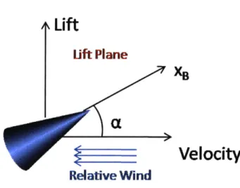
The STT control approach dictates the motion of the vehicle body by orienting the nose of the body in a particular direction relative to the velocity vector. By orienting the body in this way, the vehicle is able to direct the aerodynamic forces in a desired direction. Unlike asymmetric vehicles, the roll attitude (about the nose) of this vehicle will have no effect on the direction or magnitude of the aerodynamic force since the relative wind pressure acting perpendicular to the nose axis exhibits the same force independent of which vehicle side is facing it. The lift force is directed in a plane spanned by the velocity vector and the nose pointing vector called the lift plane. The vehicle will turn by orienting the vehicle attitude (and, therefore, lift vector) in a particular direction relative to the velocity vector. The images in Figures 1-2 and 1-2 depict the necessary attitude of the vehicle for making a turn toward the left. Figure 1-2 shows the attitude of the vehicle within the lift plane while Figure 1-3 shows the range of allowable attitude pointing directions relative to the velocity vector. The resultant lift force is denoted as

L, the angle of attack is denoted as a, and the lift bank angle is denoted as a. Also, the

displacement of the nose vector from the velocity vector in the vertical plane is defined as the pitch channel and the displacement in the horizontal plane is defined as the yaw

channel [10]. The lift bank angle determines the radial direction relative to the velocity

vector in which the attitude points, while the angle of attack determines how far along that direction the nose attitude is pointed. A particular attitude is shown within this

(29)

range that serves to turn the vehicle toward the left with the maximum angle of attack values, amax.

Lift

Lift Plane

xB

Velocity

Relative

Wind

Figure 1-2: Relationship Between Attitude And Lift In The Lift Plane

Notice in Figure 1-2 and 1-3 that the lift can be resolved into a component in the vertical plane, L cos a, and a component in the horizontal plane, L sin a, dependent on the lift bank angle. While the vertical component affects the in-plane motion of the vehicle, it is the horizontal component that creates out of plane motion and turns the vehicle. The vehicle is essentially generating lateral force by allowing the relative wind to push it one way or another, so the vehicle can be thought of as slipping, or skidding, in a direction when it executes a turn. The goal of STT control is to direct the correct amount of horizontal lift using pitch and yaw control that obtains the desired turning while still satisfying the in-plane motion.

In contrast, the bank-to-turn (BTT) control approach directs the lift force using lifting surfaces (e.g. wings) that are fixed to the body in a particular orientation. For vehicles using this approach, there is a preferred body vertical direction that points perpendicular to the lifting surface and a body side direction that points along the lifting surface in a direction perpendicular to the body nose and body vertical. While the STT approach relied on relative wind exerted against the vehicle body to generate aerodynamic force, the BTT approach primarily relies on the lifting surface, which exhibits a much larger reference area and force coefficient than the body. Therefore, the majority of the lift force will be directed perpendicular to the lifting surface and the lift direction may be changed

(30)

Locus Of Possible

Locations For xB With

a,,

Pitch Channel

Region Of All Possible x, Relative To The Velocity Vector

Figure 1-3: Relationship Between Lift Velocity Vector Direction

And Attitude As Observed By Looking Along The

Lcoso

Vertical

Plane

XB (into page) Yaw Channel

(31)

by changing the roll attitude of the vehicle. The remaining component of aerodynamic force due to pressure exerted on areas of the vehicle body other than the lifting surfaces is resolved as a sideslip force that acts in the side direction. Thus, the vehicle banks (or rolls) about the roll axis in order to divert the lift force in a desired turning direction.

It is important to note that the definitions of body vertical direction and body side direction are not applicable to the STT vehicle due to symmetry. For BTT vehicles, the

body roll angle, v, is used to defined the orientation of the body vertical direction relative

to the local vertical plane. While lift is often split up into a vertical lift component, Lv, in the body vertical direction and a sideslip force component, Ls, in the body side direction for BTT vehicles, it cannot defined as such for STT vehicles. The only analogous definitions for an STT vehicle are the pitch channel and yaw channel directions. Figure 1-4 illustrates a typical BTT vehicle, as observed from the aft, for comparison to the STT approach. In particular, the difference between the lift bank angle and the body roll angle should be noted. While the lift bank angle describes the direction of the lift vector relative to the vertical, the body roll angle describes the roll attitude of the vehicle body.

Notice that the STT and BTT control methods require different maneuvers to achieve the desired turning. The STT control method must pitch and yaw the nose vector to a desired position before the desired accelerations are obtained while BTT control can simply roll without changing the nose vector to obtain the desired acceleration. However, BTT control strategies suffer from increased complexity due to the coupling of the roll, pitch, and yaw channels [10]. Therefore, a STT control model is used for the symmetric reentry vehicle in this study.

(32)

Vertical

I

IPlane

I

I I I I I I

L

"

Velocity Vector Fuselage Wing

Figure 1-4: Depiction Of A Bank-To-Turn Vehicle, As Seen From Behind The Vehicle Tail

(33)

1.3 Mission Planning Considerations

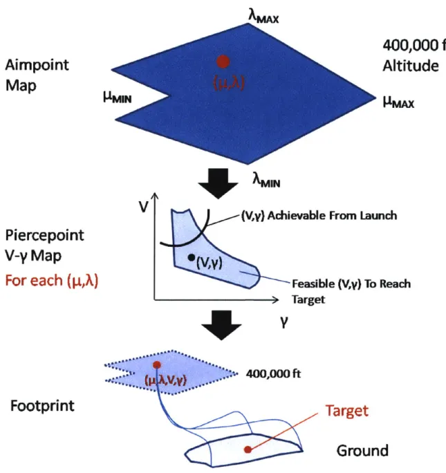
Planning for the new rapid, long range mission requires a completely new set of tools and approaches. The fundamental question for the mission planner to consider is where to aim the launch vehicle such that the reentry vehicle can safely and accurately reach its target while satisfying all necessary flight constraints. The answer to this question is influenced by a variety of complex factors, including environmental perturbations, vehicle dynamics and control authority, mission constraints, flight path constraints, and navi-gational performance. A clear and concise method for depicting the vehicle capabilities associated with each choice of aimpoint is desired. This thesis will discuss the concept of an Aimpoint Map, which represents the locus of all points at the reentry interface that can be reached by the launch vehicle and from which the reentry vehicle can reach the target. The reentry interface is chosen in this problem to occur at an altitude of 400,000 feet, since the atmosphere first begins to have an effect on the vehicle motion below this altitude. The goal of this thesis is to understand the scope of the Aimpoint Map and investigate specific properties of the Aimpoint Map related to the vehicle maneuvering capabilities.

The Aimpoint Map is defined as the collection of latitude (A) and longitude (p) points at an altitude of 400,000 feet through which a boost-through-reentry trajectory can be flown that satisfies all terminal and path constraints for both the launch and reentry portions of flight. At each point (p,A) in the Aimpoint Map, there exists a collection of velocity magnitude and flight path angle pairs (V - -y) that can both be obtained

from launch and used as valid reentry conditions for maneuvering to the target. Let the space of all such V - -7 pairs at a given piercepoint in the Aimpoint Map be defined as the

Piercepoint V-'y Map for the given piercepoint. For all reentry points within the Aimpoint

Map, at least one V - -/ pair must overlap between the launch V - y pairs and the reentry

V - 7 pairs to ensure the validity of a boost-through-reentry trajectory that flied through a particular (p,A) point. Some points in the Aimpoint Map may have many more V--y pairs than other points, suggesting that these points are more robust to uncertainties in the vehicle flight. Furthermore, given a chosen point in the Aimpoint Map and a chosen

(34)

V - y pair in the Piercepoint V--y Map, a footprint of reachable landing locations exists

which contains the target of interest. Undurti [1] demonstrated the computation of these footprints for a variety of reentry vehicles in his work. Therefore, the work presented here will focus on demonstration of the Aimpoint Map and the Piercepoint V-7 Map. These concepts are illustrated in Figure 1-5. This goal of this thesis is to demonstrate the properties of such mission planning maps for the new rapid, long range mission.

(35)

Aimpoint

Map

Piercepoint

V-y

Map

For each (i,A)

VIMIN

400,000 ft

Altitude

VIMAX

AMIN

(V,y) Achievable From Launch

Feasible (V,y) To Reach > Target

Footprint

_Target

Ground

Figure 1-5: Depiction Of Potential Trajectory Planning Concepts For The New Rapid, Long Range Mission

1.4 Trajectory Optimization

Boost-through-reentry trajectory optimization is the primary method used to investigate the complex mission planning concepts described in the previous section. A variety of trajectory optimization tools exist today that exhibit different approaches to the opti-~.;;ii;;;;;~~'..-'~

(36)

mization problem. This section will briefly describe the fundamental differences between available approaches and explain which approach is best for solving this problem.

Trajectory optimization describes a variety of methods -and approaches for determining

a vehicle trajectory that optimizes a chosen performance index subject to a set of dynamic, path, and boundary constraints. It is founded upon the principles of optimal control, in which a set of controls is chosen to influence an evolving system state in some optimal manner. Optimal control problems are particularly challenging optimization problems because they almost always involve constraints in the form of differential equations. These constraints require that the system state evolves according to some fundamental law of motion over time. For the boost-through-reentry maneuvering mission described above, these constraints ensure that the vehicle motion is governed by Newton's Second Law over the entire flight.

The trajectory optimization problem can be approached in many ways. The desired solution is one that is both optimal and feasible. Optimality asserts that the performance index is at a minimum value while feasibility asserts that all constraints are satisfied. Many different approaches are available for verifying both the optimality and feasibility of an optimal control problem. Two main classifications of approaches to solving optimal control problems exist today: direct methods and indirect methods [7].

Most complex optimal control problems are solved numerically using nonlinear pro-gramming (NLP) principles. Both direct and indirect methods perform iterations of Newton's methods to solve for a finite set of unknowns [7]. The difference between them lies in the particular application of Newton's method. Indirect methods use Newton's method to solve a multipoint boundary value problem (BVP) that is formulated using Pontryagin's Minimum Principle and the Calculus of Variations. Any solution to the BVP will satisfy the first-order optimality conditions, which are the necessary conditions de-rived from the Calculus of Variations. In contrast, direct methods use Newton's method to iteratively conduct a search for the solution that reduces the performance index at each iteration until a minimum is converged upon [7]. At every Newton iteration, direct methods must compute gradients in an effort to move in a direction that moves closer to the minimum performance index. Thus, indirect methods seek to influence the

(37)

perfor-mance index indirectly through a set of derived necessary conditions while direct methods perform iterations that directly influence the performance index at each time step [7].

The fundamental drawback to using indirect methods, as compared to direct meth-ods, is that a new set of necessary conditions must be analytically derived for each new optimization application. This can be difficult and time consuming for complicated dy-namical systems, such as the vehicle investigated in this study. In addition, indirect methods typically require better initial guesses than direct methods and have difficulty solving problems with path inequality constraints [7]. However, as mentioned before, solutions to indirect methods are guaranteed to satisfy first-order optimality conditions and do not require any additional check on feasibility and optimality [7], whereas direct methods typically do not provide a method for checking the optimality conditions. Di-rect methods can also suffer from high computation costs and inaccuracies when analytic gradients are not available. For very complicated optimization problems, such as the problem considered in this study, gradients must be computed numerically using finite difference approximations, representing a source of potential inaccuracies and increased computation time.

Among direct and indirect methods, shooting methods and collocation methods are the most popular. Direct and indirect variants exist for both shooting and collocation meth-ods. Shooting methods approach the problem by solving an initial value problem within each Newton iteration. Direct shooting propagates the trajectory to an end condition, evaluates the constraints and performance index, and returns these values to the Newton iterator for a search towards the minimum performance index that satisfies all flight con-straints. Similarly, indirect shooting propagates the necessary conditions to the end state, evaluates the constraint residuals, and iterates until the BVP is solved. Shooting meth-ods suffer from high sensitivity to small perturbations early in the trajectory. Since these methods iterate over values evaluated at the end of a propagation, small changes early in the propagation can have very large, nonlinear effects at the terminal boundary. Ad-ditionally, these methods are only reasonable for problems containing a small number of variables since the finite difference approximations for the gradient are obtained through a numerical integration of the trajectory [7]. If many gradients must be computed and

(38)

checked for each Newton iteration, the problem can become very time consuming. Many commercial optimizers, such as POST, utilize the direct shooting approach for a variety of problems while indirect shooting has primarily been used to solve very specialized cases due to sensitivity issues [7].

Collocation methods solve the trajectory optimization problem by discretizing the tra-jectory into a set of grid points, or nodes [7]. By discretizing the tratra-jectory, collocation methods transform the original trajectory optimization problem into a discrete NLP prob-lem where the variables are the states and controls at each node point. At each node, the trajectory states must be chosen such that they satisfy the differential equations gov-erning the motion of the state, as well as other boundary and path constraints. This approach differs significantly from the shooting method, which numerically integrates an entire trajectory during each Newton iteration. The NLP approach requires no numerical integration. Rather, a series of iterations are performed to choose the trajectory states at the nodes that minimize the performance index. Indirect collocation seeks to satisfy the dynamics of the BVP at each node while direct collocation seeks to satisfy the trajec-tory dynamics at each node while iterating over the performance index. Both approaches have the disadvantage of solving a NLP problem with a very large number of variables. However, many direct collocation methods are able to increase computational efficiency by exploiting the sparsity of the gradient matrices [7]. Unlike all of the other methods mentioned, direct collocation methods have the distinct advantage of being able to solve problems with path inequalities without needing to define portions of the trajectory where each path constraint is active and inactive a priori [7].

The exact spacing of the nodes has been an active area of research in optimization theory. It is advantageous to choose a spacing for the nodes that allows for the best polynomial approximation of the trajectory states by values evaluated at the node points [12]. Pseudospectral (PS) methods are direct collocation methods that choose the nodes to be located at the Legendre-Gauss-Lobatto (LGL) points, which provide the optimal node spacing for constructing Legendre polynomial approximations [6] [12]. Pseudospectral methods are increasingly popular for numerically solving optimal control problems because they offer an exponential convergence rate for the approximation of analytic functions [19].

(39)

For the optimal control problems addressed in this thesis, a direct collocation method using Pseudospectral discretization will be used. This approach is chosen because the problems in this thesis involve a variety of complex path and terminal constraints that cannot be solved easily with other approaches. In addition, a variety of different metrics will be optimized in these problems, which are readily achieved with direct methods using a single formulation, but require many different formulations for indirect methods. Fur-thermore, the LGL node spacing provides superior convergence properties [19]. DIDO, a MATLAB application for solving smooth and nonsmooth hybrid optimal control prob-lems using Pseudospectral methods, will be used to solve the optimization probprob-lems in this thesis [6]. DIDO will numerically solve an optimal control problem involving a dy-namic model of the vehicle and a formulation of the flight constraints. These models will be developed in the coming chapters for application to DIDO.

1.5 Thesis Overview

The goal of this thesis is to investigate properties of potential mission planning concepts for the new long-range, high-precision boost-through-reentry mission. Chapter 2 will develop a set of relevant coordinate frames and parameters for describing the complex boost and reentry motion of the vehicle relative to a rotating, spherical Earth. In chapter 3, a six degrees-of-freedom (6DOF) vehicle model will be derived for governing the translational and rotational motion of the vehicle in flight. Chapter 4 will discuss the formulation of the optimal control problem, while chapter 5 and chapter 6 will discuss vehicle models for boost and reentry. Finally, chapter 7 ties together the boost and reentry portions of flight with the computation of a representative Aimpoint Map.

(40)

(41)

Chapter 2 Coordinate Frames

This chapter will develop the framework for describing the motion of a manuevering reentry vehicle moving at hypersonic speeds in the Earth's atmosphere. A variety of coordinate frames will be developed to adequately describe the translational and rotational motion of the vehicle including:

* Earth Centered Inertial Coordinate Frame (ECI)

* Earth Centered Earth Fixed Coordinate Frame (ECEF) * Reference Plane Coordinate Frame (REF)

* Up-Downrange-Crossrange Coordinate Frame (UDC) * Velocity Coordinate Frame (V)

* Non-Rolling Body Coordinate Frame (B)

The goal of this chapter is to develop a series of coordinate systems that define relevant parameters for position, velocity, and attitude determination and exhibit uniform validity for both endo-atmospheric and exo-atmospheric flight regimes.

2.1 Earth Centered Inertial (ECI) Coordinate Frame

The Earth Centered Inertial Coordinate Frame is an inertial reference frame fixed at the center of the Earth. An Earth centered inertial frame can have many different orientations,

(42)

provided that it is fixed to the center of the Earth and non-rotating. A commonly used inertial frame is the J2000 frame, a geocentric inertial coordinate frame that is defined with reference to the Julian Epoch of January 1, 2000. The z-axis, 2i, points along the Earth's rotation axis through the Geographic North Pole, defined as 90 degrees North Latitude. The x-axis, RI, points in the direction of the Vernal Point, defined as the unit vector pointing from the center of the Earth to the Sun location during the Vernal Equinox (referenced to the Julian Epoch). The third axis, yI = 2I x RI, completes the right-handed coordinate system. By definition, the I1 - YI plane is aligned with the Earth's equator,

defined as 0 degrees latitude.

Z,

X,

Equator

VI

Figure 2-1: Earth Centered Inertial Coordinate Frame

The ECI frame translates with the Earth as it revolves around the Sun, but does not rotate with the Earth. The position and velocity of the vehicle in this frame, therefore, are inertial and are defined relative to a fixed orientation in space. Since the work in this study is concerned with motion relative to the Earth's surface, additional reference frames are required to adequately define Earth-relative motion with continually changing local vertical and local horizontal planes.

(43)

2.2 Earth Centered Earth Fixed (ECEF) Coordinate

Frame

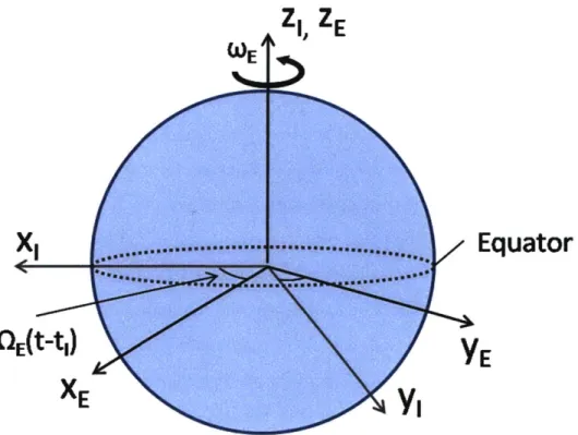
The Earth Centered Earth Fixed Coordinate Frame is an Earth-fixed rotating frame that is positioned at the center of the Earth and rotates about the Earth's rotation axis. The Earth's rotation axis is assumed to rotate with a constant rotation rate, QE, of 7.292115 x 10- 5 radians per second, neglecting precession and nutation effects. The x-axis, kE, points to 0 degrees latitude, 0 degrees longitude at all times. The z-axis, _ZE, is aligned with the Earth's rotation axis and the y-axis, YE = 2E X kE, completes the

right-handed coordinate system. The X^E - YE plane defines the Earth Equatorial Plane with ZE pointing perpendicular to the Equator and through the Geographic North Pole.

At any time t, the transformation from the ECI frame to the ECEF frame involves a rotation of QE(t- tI), where t₁is the reference time when the -I₁and XE axes were last aligned. Zl, ZE WE

X

~.

Equator

QE(t-tJ)

E

XE

|Y

Figure 2-2: Earth Centered Earth Fixed (ECEF) Frame

(44)

cosQE(t - t1) in E (t - ) 0 T = - sin E(t - t) COS QE(t--t ) 0

0 0 1

The angular velocity vector of the ECEF frame with respect to the ECI frame is

EI EZI = QEZE

2.3 Reference Plane (REF) Coordinate Frame

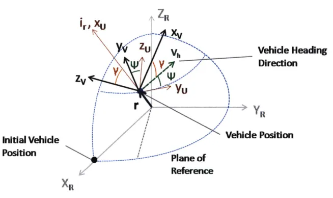
The Reference Plane Coordinate Frame is an Earth-fixed, rotating frame positioned at the center of the Earth with axes positioned along a chosen plane of reference passing through the center of the Earth. It rotates with the same rotation rate as the ECEF frame, and therefore is observed to be fixed relative to the ECEF frame. The purpose of the Reference Plane Coordinate Frame is to provide a frame that measures vehicle motion relative to a chosen plane of reference. In this frame, the Equator, used as a plane of reference in the ECEF frame, is replaced by a new plane of reference. This plane of reference can be defined by an initial vehicle position and heading or by a plane containing a launch point and a landing point. Ikawa [2] derives equations of motion for a vehicle traveling relative to a plane of reference defined by the initial heading of the vehicle. In this study, the plane of reference will be defined as the plane containing both the initial location and the final destination. The use of such a coordinate frame can be particularly advantageous when when attempting to measure maximum downrange and maximum crossrange capabilities from a plane of interest. In addition, the use of a reference plane can avoid singularities that occur when angular values (e.g. latitude) approach 90 degrees. The new variables defining the vehicle position in this frame will be defined as relative longitude, p, and

relative latitude, A, as measured relative to the plane of reference and the initial vehicle

location.

The axes are transformed from the ECEF frame such that the x and y axes lie in a

(45)

inl--SZE

XE

*

a

Initial Vehide

SLocation

Equator

YE

Plane of

Reference

Figure 2-3: Reference (REF) Coordinate Frame

chosen plane of reference and the z axis points perpendicular to this plane. The x-axis,

XR, points towards the initial vehicle position, while the z-axis, ZR, is directed normal

to the plane of reference and the y-axis, YR = R x ^R, completes the right-handed coordinate system.

The initial vehicle position and plane of reference can be described in terms of the three angles (o, io, and 00. The first angle, (o, describes the nodal point shift of the plane of reference, defined as the positive angle measured counter-clockwise along the Equator from the RE axis to the nodal point of the reference plane, iN. The unit direction of nodal point is defined as

1N - ZE X ZR

can then be computed as the

angle between _|2E_X _^RjXE and i

4o can then be computed as the angle between X-E and iN:

(46)

4Io = cos- ' IN " XE

JiNJI^E1E

The second angle, io, defines the inclination of the plane of reference with respect to the Equator. This is defined mathematically as

o = COS1 ZR ZE

so = cos Z

The third angle, 0o, defines the initial vehicle angular position along the plane of reference as measured from the node, iN Similarly, 0o can be defined mathematically as:

0 O-1 IN 'XR

0o =

cos-iN HXR

When io, 00, and 1o are equal to zero, the plane of reference becomes the Equator and

p and A represent the longitude and latitude location of a point on the Earth. With the

use of the REF coordinate frame, the Earth-relative vehicle position can now be expressed relative to any arbitrary reference point and reference plane.

The REF frame can be obtained from the ECEF coordinate frame through a series of three rotations as follows:

1. Rotation about the iE axis by (o.

2. Rotation about the iN vector by io.

3. Rotation about the 2R axis by 00.

Thus, the transformation matrix from ECEF coordinates to REF coordinates is defined

cos 00 sin 00 0 -sin0 0 cos00 0 0 0 1 0 0 cos io sin io - sinio cos io cos Qo sin Q₀ 0 -sin o cos o 0 0 0 1

:I _ 3:_~ii~\_i ij/;i ^i___ ___ ~-~-li---~-l l__~__r ~ ~ l~_ i ---~--~- I^ ICIC~X ~ ILIIL~ii ii~-l~ii-ii ii--i-- Il---i----l- r-* ... ... .l*

Boost through reentry trajectory planning for maneuvering reentry vehicles

Boost Through Reentry Trajectory Planning For

Maneuvering Reentry Vehicles

OCT

13 2009

LIBRARIES

ARCHIVES

P/>

SJohn

Boost Through Reentry Trajectory Planning For Maneuvering

Reentry Vehicles

by

Matthew James Abrahamson

Abstract

Acknowledgments

3Matthew

J. Abralmson

Date

Contents

List of Figures

List of Tables

Chapter 1

Introduction

1.1

Maneuvering Reentry Vehicles

-1.2

Skid-To-Turn Control

Lift

xB

Velocity

Relative

Wind

a,,

Vertical

Plane

Vertical

I

IPlane

I

L

"

1.3

Mission Planning Considerations

Aimpoint

Map

Piercepoint

V-y

Map

For each (i,A)

400,000 ft

Altitude

Footprint

Target

Ground

1.4

Trajectory Optimization

1.5

Thesis Overview

Chapter 2

Coordinate Frames

2.1

Earth Centered Inertial (ECI) Coordinate Frame

X,

Equator

VI

2.2

Earth Centered Earth Fixed (ECEF) Coordinate

Frame

X

~.

Equator

QE(t-tJ)

E

XE

|Y

2.3

Reference Plane (REF) Coordinate Frame

XE

*

a

_Target