Analyzing Multiple Product Development Projects Based
On Information and Resource Constraints
Ali Yassine+ & Tyson Browning* +
Massachusetts Institute of Technology
*
Lockheed Martin Aeronautics Company
Abstract
Product development (PD) and engineering design processes are often characterized by the
information flowing among activities. In PD, this flow forms a complex activity web—a process
that can be viewed as a complex system. Most literature on the subject of information flow in
PD focuses on a single project, where precedence information constraints (based solely on
necessary information and possible assumptions) determine the execution sequence for the
activities and the resultant project lead-time. In this paper, we consider multiple PD projects that
share a common set of design resources. Especially in this setting, precedence information
availability is insufficient to assure that activities will execute on time. We extend the
information flow modeling literature by including resource availability. We model several PD
projects as a portfolio, where activity execution is based on both information and resource
availability. We demonstrate the effects of accounting for resource constraints on both
individual projects’ and portfolio lead-time distributions.
+ Corresponding author: MIT, CTPID, Rm. E40-253, Cambridge, MA. 02139. Tel. (617)258-7734, Fax (617)452-2265, E-mail: [email protected]
1. Introduction
A fast product development (PD) process can provide a source of competitive advantage
[17, 23]. The speed of a PD process is largely influenced by how it is structured and managed.
However, managing PD projects has always been a challenge in the manufacturing industry due
to the unpredictable nature of engineering design, where design iterations are a pervasive
phenomenon. Successful project completion requires repetition and updating of many
development activities. Iteration influences PD cost and schedule immensely. Even though
particular iterations are not necessarily known with certainty prior to project execution, a skilled
manger (equipped with the right tools) can identify many potentially iterative development
activities and plan accordingly. Understanding the web of information flow in a project can help
identify potential iterations. Unfortunately, many PD managers fail to plan for iterations;
consequently, PD projects incur schedule and cost overruns [2, 5] - often forcing them ultimately
to sacrifice scope or to fail.
The PD process management problem is compounded when companies manage a
portfolio of PD projects at once. In a multi-project PD environment, organizations tend to
micromanage their PD portfolio [9, 11, 26]. That is, managers direct attention to one project at a
time and allocate resources accordingly, ignoring the interactions and interdependencies between
projects. Instead, scarce development resources should be managed from a PD system
perspective and allocated to maximize the value of the whole portfolio.
Researchers have suggested many models, tools, and techniques to help managers plan
and control PD projects more effectively [22]. One such tool is the Design Structure Matrix
(DSM), which provides a means of representing a complex system (such as a process) based on
its constituent elements (activities) and their relationships (information flow). DSM-based
literature focuses on a single project and the flow of information within. In the DSM
methodology, precedence constraints based on information dependencies determine the optimal
execution sequence for a set of activities. In this paper, we introduce an important, new
constraint, resources, into the DSM analysis. When we consider multiple, simultaneous
development projects within an organization (sharing a common set of design resources), the
availability of predecessor information is insufficient to assure that activities will be executed on
time. We address resource availability through a project portfolio plan that constrains activity
execution based on both information and resource availability.
This paper has two primary purposes. First, we demonstrate that a DSM model can
meaningfully represent both multiple PD projects and resource constraints. Second, based on
this extension, we develop a simulation model of multiple PD projects, which results in the
development of performance measures for each individual project and for the portfolio as a
whole.
Resource constraints force choices about which activities to support at a given time. To
make this decision, we define a preference function that determines the insertion points of
resource constraints in an aggregate DSM representing the entire portfolio of projects. The
preference function is used to simulate the mental decision-making process that resources (i.e.,
project participants or processors) go through when dealing with multiple projects, thereby
allowing us to simulate the execution of activities in a multi-tasking environment.
The simulation model presented in this paper provides organizations with an analytical
tool to analyze the impact of multi-tasking and resource allocation policies on project and
portfolio lead times. This will ultimately assist organizations in the development of better
The paper is organized as follows. Section 2 surveys the literature for existing single and
multi-project modeling and management techniques, and Section 3 reviews the DSM
methodology. In Section 4, we introduce several modeling constructs that are essential for the
building the multi-project model. Section 5 describes how the model is simulated, and Section 6
provides an example with simulation results and sensitivity analysis of some important model
parameters. Finally, Section 7 summarizes and concludes the paper.
2. Literature review
A review of project management literature in general, and PD management in particular,
reveals the existence of numerous models addressing both single and multiple projects. Perhaps
the most visited problem is the well-known resource-constrained-project-scheduling problem
(RCPSP) resulting in many exact solutions (all based on a 0-1 integer linear programming
formulation) and numerous heuristic procedures. Brucker et al. [6] provide a recent,
comprehensive review. A natural extension to the RCPSP deals with multiple projects [13]. The
major deficiency of the RCPSP formulations in dealing with PD management problems is their
inability to address feedback loops that result in the rework of some activities.1 This literature
differs from our paper in a major way. While RCPSP techniques seek to optimize the scheduling
of activities based on generic precedence and resource constraints, we are evaluating project lead
times using predetermined and fixed project architectures and schedules based on a fuller
characterization of information flow.
Other researchers suggest the use of queuing networks [20], Petri nets [14], or stochastic
dynamic programming [3] to capture the stochastic nature of information flows in PD processes
1 Methods such as GERT (Graphical Evaluation and Review Technique) addressed this deficiency by accounting for uncertainties in the sequence of activities in the project (Neumann, 1990). However, GERT charts provide poor visualization of the full information flow in a design process and do not account for multiple projects.
and build corresponding simulation models. For instance, Adler et al. [1] analyze an activity
network allowing for reentrant queues (to model rework) using a discrete event simulation. The
simulation allowed them to identify bottleneck activities and several other process
characteristics. Our paper is closely related to this research stream, but contrary to these models
that assume stochastic arrivals of activities, instead we assume, at the outset of the simulation,
that the number of projects and activities are planned; uncertainty is only found in rework
occurrence and activity duration.
Simulation of PD projects has also been used in computational, micro-contingency
organization theory by Levitt et al. [15]. This research relates to our work even though we focus
on project management and Levitt’s research focuses on organizational design. Levitt’s research
employs simulation techniques to understand and predict the effects of alternative organization
and work process designs on project performance in complex organizations. In order to simulate
a project in an organizational setting, Levitt and his research team define a set of attributes that
describe the project activities, the project participants, communication between participants, and
the organizational structure. Similarly, our simulation employs attributes for activities, projects,
and personal preferences to build the processor preference function. We are interested in
understanding how the preference dynamics of PD participants involved in multiple projects
influences PD performance.
Another related research stream is multi-criteria methods for project selection [4], usually
in R&D environments [16, 24]. These techniques utilize a set of measures to evaluate each
project within a portfolio and then calculate a weighted utility measure for each. This allows the
prioritization of the projects. However, this approach utilizes little if any information about the
efficiency of each project’s PD process architecture. In this paper, we utilize a similar technique
simulation, thus combining these multi-criteria techniques with information flow simulation
techniques.
Finally, our model relates to the critical chain methodology developed by Goldratt [11].
Goldratt established a set of generic rules to improve multi-project performance that include, in
addition to buffer management, avoidance of resource multitasking. He conjectured that
resource multitasking results in lead time increase due to the lack of clear priority, but he did not
show how to measure these priorities in order to eliminate possible resource confusion. In this
paper, we explicitly account for different priorities in a multitasking environment.
3. The Design Structure Matrix (DSM) Model
DSM-based models have been used to represent the technical relationships between
design activities in complex PD projects. The simplest DSM model of a design project is a
binary, square matrix with n rows and columns, and m non-zero elements, where n is the number
of activities and m is the number of dependencies between the activities. Activity names are
listed down the left side of the matrix as row headings and across the top as column headings in
the same order. If activity i depends on activity j, then the value of element ij (row i, column j) is
unity (or marked with a “n”). Otherwise, the value of the element is zero (or left empty). In the
binary matrix representation, the diagonal elements of the matrix do not have any interpretation
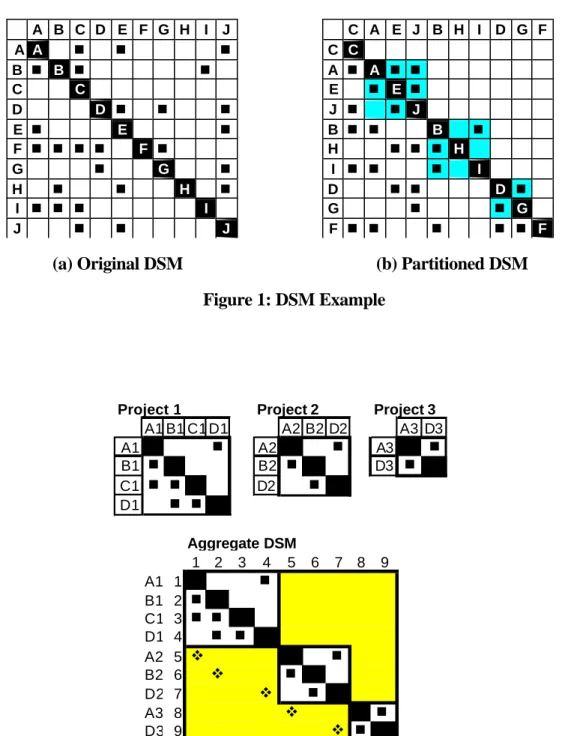
in describing the project, so they are usually either left empty or blacked out. Sample DSMs are
shown in Figure 1. In this convention, subdiagonal elements in the DSM represent feed-forward
information flows among the activities and superdiagonal elements represent feedbacks.2
Feedback information flow captures much of the iteration and rework potential in a design
project.
2
The DSM model can be used to determine an improved sequence for the design activities
[10]. Reordering the activities within the DSM can eliminate or reduce the number and impact
of feedback loops in the project. Partitioning3 is the process of resequencing the DSM rows and
columns such that the new DSM arrangement contains minimal feedback marks—i.e., towards
lower-triangular form. For complex engineering projects, it is highly unlikely that mere row and
column manipulation will achieve a complete lower-triangular form. Therefore, the analyst’s
objective changes from eliminating the feedback marks to moving them as close as possible to
the diagonal (this form of the matrix is known as block triangular). In doing so, fewer activities
will be involved in iteration cycles, resulting in a faster and more predictable development
process. Figure 1b shows the result of partitioning the DSM in Figure 1a.
The partitioned DSM (Figure 1b) shows the existence of three iterative blocks (the
highlighted squares along the diagonal): A-E-J, B-H-I, and D-G. The activities included in a
block are coupled and are candidates for iteration. For example, consider the execution of the
activities within block (B-H-I) and assume that all activities prior to activity B are completed.
Activity B requires inputs from activities C and A (already completed) and activity I, which is
not completed yet. Therefore, activity B starts with missing information (perhaps making a
guess on the value required from activity I). Once activity B is completed, it delivers its output
information to both activities H and I. When activity I finishes its original work, it delivers its
output information back to activity B (as represented by the feedback mark in the block). At this
point, activity B reevaluates its earlier results in light of the new information received; thus,
activity B might or might not need to perform another iteration (some rework). If iteration is
performed by activity B, then we refer to it as first-order rework. Due to the coupled nature of
the block, second-order rework is also possible. That is, if activity B, which feeds activities H
3
and I, is reworked, then there is a chance that either activity H, activity I, or both will also need
to be repeated. This is called second-order rework. If activity I is reworked, then the iterative
process, described above, might be repeated several times, resulting in higher-order rework.
Several extensions to the base DSM model have been proposed to include more
information in the matrix (e.g., [5, 7, 28]). Reviewing all of these extensions is outside the scope
of this paper. However, one such extension directly related to this paper is a method to perform
Monte Carlo simulation on the DSM [28]. The DSM simulation model characterizes the design
process as being composed of activities that depend on each other for information. Changes in
that information cause rework. As discussed earlier, rework in one activity can cause a chain
reaction through supposedly finished and in-progress activities. Activity rework is a function of
rework risk, which combines the probability of a change in inputs and the impact this change
might have on the dependent activities. The impact measure used in the simulation represents
the fraction of the original work (i.e., activity duration) that needs to be repeated or reworked.
Both probabilities and impacts are numbers between 0 and 1 and they replace the marks in the
binary DSM. Thus, the simulation model is represented by two identical DSMs, one containing
probabilities of information change and the other containing the impacts of change. In the
probability DSM, the superdiagonal marks are replaced by first-order rework probabilities, and
the lower-diagonal marks are replaced by second-order rework probabilities. The simulation
also accounts for stochastic activity duration by using three point estimates (optimistic, most
likely, and pessimistic) to form a triangle distribution. In this paper, we utilize a similar
simulation; however, we expand the simulation into multiple projects and include the impact of
4. A Framework for Multi-Project Simulation
This section discusses three modeling constructs employed: aggregate DSMs, project
queues, and processor preference functions.
4.1 The Multi-Project DSM Model
In this subsection, we discuss the extension of the single-project DSM to include multiple
projects and resource constraints. We refer to the multi-project DSM as the aggregate DSM.
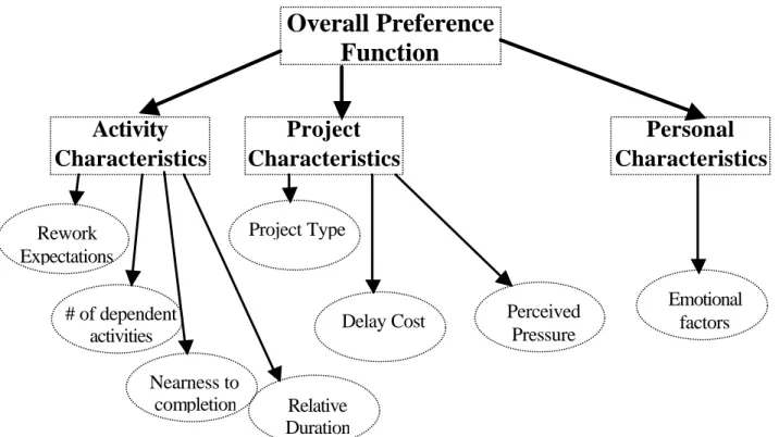
Building the aggregate DSM is best illustrated through a simple example. Consider three
development projects occurring simultaneously (projects 1, 2, and 3) and involving four
development resources/processors (A, B, C, and D), as shown in the top part of Figure 2.
Processor A is assigned to all projects as depicted in the Figure by A1, A2, and A3. Processor B
is assigned to projects 1 and 2 as depicted in the Figure by B1 and B2. The same representation
holds for processors C and D.
The aggregate DSM, shown in the lower part of Figure 2, combines the DSMs for each
project. The square marks (“n”) inside the aggregate DSM represent information constraints,
while the diamond marks (“v”) represent resource constraints. Note that the diamond marks
shown in the figure represent only one possible resource constraint profile. The arrangement
shown assumes that activities in project 1 are preferred to activities in project 2, and activities in
project 2 are preferred to activities in project 3. For example, the diamond mark in row 5 and
column 1 conveys that A2 depends on A1 finish for its execution. Inserting this mark in row 1
column 5, instead, would reverse the resource dependency. In general, if a processor is assigned
to p projects, then there are (p!) possible priority profiles for that processor.
The aggregate DSM provides managers of multiple projects a simple snapshot of the
within projects and across multiple projects, while explicitly accounting for resource contention.4
Partitioning the aggregate DSM reveals an improved information flow and clear resource
prioritization across the whole PD portfolio as compared to independently partitioning the
individual project DSMs.
4.2 Project Queues
Each processor can be involved in multiple activities (from the same or different
projects), but they can only work on one project’s activity at any given moment. The list of
activities from different projects is called the project queue for a processor. We will refer to each
processor’s project queue as Qi, where i is the processor index. At any time, t, Qi(t) consists of
two mutually exclusive and collectively exhaustive partitions: Ai(t) and Ii(t).
The processor’s active queue, Ai(t), contains a subset of Qi(t) that is readily available for
work (based on predecessor information availability only) at time t. The processor must choose
one of these activities to work on. The inactive queue, Ii(t), contains all other activities. Recall
that coupled activities are those activities involved in an iterative block. A work policy is used to
allocate coupled activities to either Ai(t) or Ii(t) based on how the activities are sequenced in the
DSM (the process architecture determined by partitioning). The first activities in the coupled
block make assumptions about the later activities’ inputs and are assigned to Ai(t).
4 In this paper we assume no information dependencies (only resource constraints) between projects, but the aggregate DSM can accommodate such dependencies by allowing the insertion of a combination of square and diamond marks outside the individual projects blocks.
4.3 The Preference Function
If a processor is assigned to two projects and it can perform work on either one, at a
given instant in time, the choice is made based on a preference function that includes activity,
project, and processor characteristics. The preference function addresses the following concerns:
a. When faced with a choice, which activity (in which project) should a processor work on?
b. What is the impact of the above decision on PD time?
The preference function (or priority profile) ranks the activities in processors’ active
queues, so that the activity with the highest priority is selected to work on. Preference or priority
is a function of activity, project, and processor attributes. The attribute hierarchy is shown in the
tree of Figure 3. Determining how to weight the attributes requires conducting interviews with
the processors involved in the different projects to solicit their mental value model they use when
determining activity priorities. For an extensive explanation of the method we used for building
the attribute hierarchy and selecting convenient attribute measures, the reader is referred to
Keeney’s book on value focused thinking [12]. Our preference function consists of a weighted
combination of the eight attributes listed and discussed in Table 1.
Each branch, i, in the attribute hierarchy (Figure 3) has a weight, ki, and a utility or
preference value, Ui, which is a function of the attribute level, xi. The utility functions or curves
used are shown in Figure 5. To arrive at an overall preference index for each activity, we use a
weighted sum: U(x1, …., xn) =
∑
= n i i i iU x k 1 )
( . Each utility curve is defined over [0,1], and all of
the weights are positive and sum to one, so the overall preference index is also defined over
[0,1]. Once a preference index is calculated for each activity in a processor’s active queue, the
Assessing the weight and utility curve for each attribute requires interviews with the
different processors. There are numerous assessment techniques suggested in the decision
analysis literature. Discussing all such techniques is outside the scope of this paper; however,
the interested reader is referred to [8]. The simplest technique is the direct assessment technique,
where participants are asked to score each attribute on a scale (say from 0 to 100). Then, these
scores are normalized through dividing each attribute’s score by the sum of all scores. A more
sophisticated assessment can be employed using the AHP method of pair-wise comparisons [27].
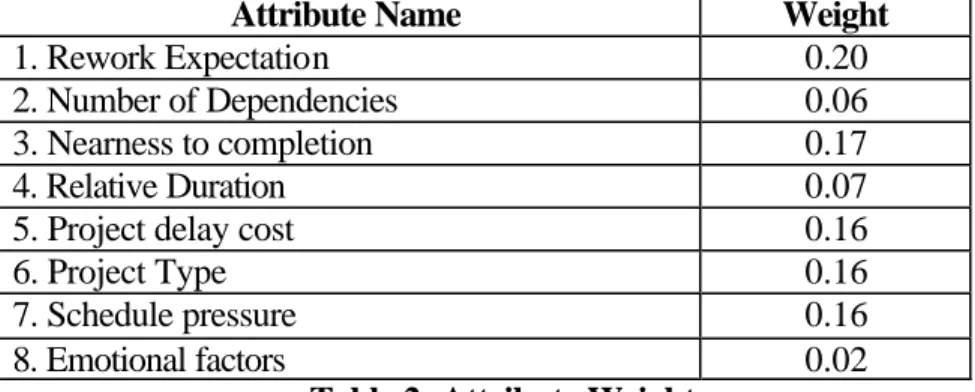
Table 2 provides the attribute weights directly assessed by conducting a set of structured
interviews with PD project managers from a chemical products manufacturing firm.5 The single
attribute utility functions shown in Figure 5 were assessed during the same interview process
using the mid-level splitting method [8].6
It is worth noting that we have run our simulations using one set of attribute weights and
the same utility curves for all the processors because we recommend conducting interviews for
their assessment in a group environment. This will eliminate any biases in the assessment
process and achieve group consensus on the attribute weights and the shape of the utility curves.
Alternatively, the model can easily be modified to allow for different weights and utility curves
for each processor; however, multiple one-on-one interviews will be required instead of the
group assessments.
5
The authors gratefully acknowledge the help of Brad Boersen, an SDM Masters student at MIT, in conducting the interviews for determining the set of relevant attributes, assessing the attributes’ weights, and soliciting the shapes of the single utility functions. 6 Initally, it might be more practical to use linear utility functions (after assessing the end points) instead of expending effort during an interview to solicit non-linear ones. After performing the first round of simulations and conducting some sensitivity analysis to determine if lead times are highly sensitive to the shape of the utility functions, then it will be worth going back to the participants to reassess their utility functions. Otherwise, linear utility functions may suffice.
4.4 Model Assumptions
a. Each project is important to somebody (no consensus on the most important project to work
on), so processors must choose which activities to work on based on various criteria.
b. There is a one-to-one correspondence between activities and processors.
c. Projects are independent except for resource constraints (i.e., all marks in the aggregate
DSM, outside of the individual project blocks, represent resource constraints).
d. Initially, switching costs / penalties are not considered. However, we later remove this
assumption by accounting for switching penalties when a processor begins working on a new
activity.
5. Simulating the Model
The simulation is implemented in a spreadsheet model using Excel Visual Basic macro
programming.7 All input information (i.e. project data and the corresponding activity details) is
entered into the Excel spreadsheet. Then, the simulation starts by executing the simulation
macros. The results of the simulation are displayed as a set of lead-time distributions for each
project and for the whole portfolio.
In our simulation, project execution is guided by a specific work policy. We use a simple
work policy that requires all predecessor activities to be completed before an activity is eligible
to begin work. However, coupled activities can begin work without inputs from downstream
activities within their block (by making assumptions about the nature of those inputs). Prior to
the beginning of the simulation, the aggregate DSM is partitioned in order to the minimal set of
coupled activities.8 Then, a nominal duration for each activity is randomly sampled from its
7
The multi-project DSM simulation program can be downloaded from <http://web.mit.edu/dsm/Tutorial/Multiple-DSMs.htm> 8
triangular distribution.9 These sampled durations are saved in a temporary vector for later use
within a single simulation run.
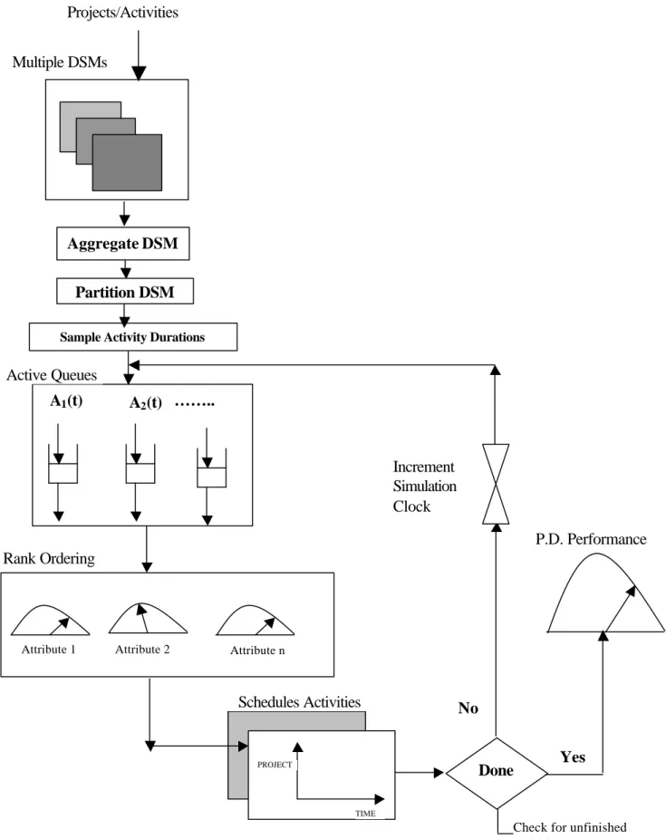
Once the DSM is partitioned and nominal activity durations are sampled, the simulation
proceeds through increments of time, ∆t.10 At each time step, the simulation must (a) determine which activities are worked on (b) record the amount of work accomplished, and (c) check for
possible rework. Determining which activities can be worked requires two steps:
a. Determine which activities are eligible to do work based only on information constraints.
Activities that have work to do and for which all predecessor activities are completed (i.e.,
for which all upstream input information is available) are eligible.
b. Assign eligible activities to their processors, thereby determining each processor’s active
queue. If any processor has more than one activity in their active queue, then the preference
algorithm is invoked to select the activity the processor will address in the current time step.
This step essentially entails temporarily inserting additional marks into the DSM that
represent processors’ preferences for eligible activities.
Each processor’s active queue is redetermined at each time step. If it is empty, then the
processor is idle. If it contains a single activity, then the processor works on that activity. If the
active queue contains more than one activity, then the preference function is invoked to
determine which activity the processor will work on. At each time step, the simulation deducts a
fraction of “work to be done” from each working activity. Finally, at the end of each time step,
the simulation macro notes all activities that have just finished (nominal duration or rework). The
macro performs another check to determine the coupled ones by inspecting the partitioned
aggregate DSM. For each one of these finished and coupled activities, a probabilistic call is
9 The triangular distribution for each activity duration is represented by the minimum, likely, and maximum duration values in the input spreadsheet
made to determine whether this activity will trigger rework for other coupled activities within its
block. If rework is triggered, then the amount of rework is determined from the impact DSM and
added to the “work to be done” on the impacted activity.
A simulation run provides a simulated duration for each project in the portfolio, and for
the portfolio as a whole. The simulation is run many times (e.g., 1000 times) to provide a
distribution of duration outcomes. A pictorial flowchart for the above algorithm is shown in
Figure 6.
6. Example
In this section we illustrate the application of the simulation model. This example
consists of three PD projects (numbered 1, 2, and 3) sharing eight development resources (named
A through H). The aggregate DSMs showing information dependencies, feedback probabilities,
and rework impacts are shown in Figure 7. The three-point duration estimates for each activity
and its deadline are shown in Table 3. Table 4 contains project-related input data such as project
type, deadline, budget, and cost of delay.
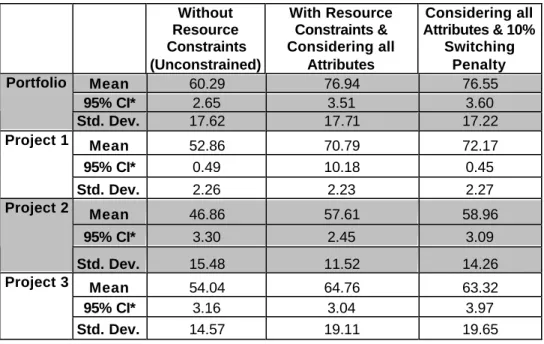
6.1 Simulation Results
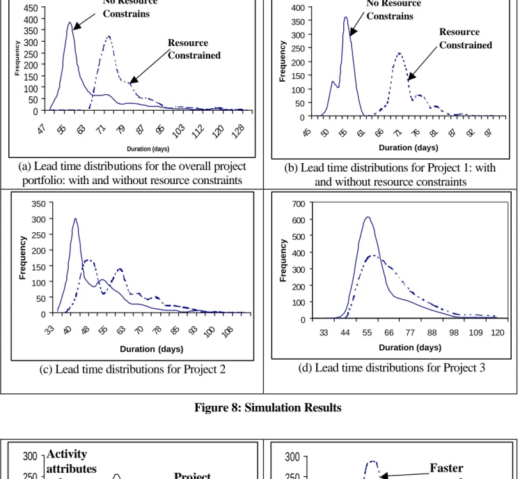
The simulation output is represented by a series of lead-time distributions as shown in
Figure 8.11 The first chart (Figure 8a) represents the development time distribution for the whole
PD portfolio. The other three charts (Figures 8b, 8c, and 8d) represent lead-time distributions for
the individual projects. The solid curves represent time distributions when resource constraints
are not accounted for—i.e., assuming unlimited resources. The dashed curves, however,
10
A discrete event simulation was considered (and could provide a superior approach) but would be more difficult to implement in a spreadsheet without substantial additional coding and/or third party software. The simple, time-advancing simulation suffices to demonstrate the insights of the model.
represent time distributions when activities compete for resources and priorities are assigned to
them based on the eight attributes discussed earlier. The shift form the solid curves to the dashed
curves represents the strength of resource contention and the degree of error in information flow
models that do not account for resource contention. For example, inspecting Figure 8d shows
that project 3 was minimally impacted by the resource constraints as compared to projects 1 and
2. Similarly, inspecting Figure 8b reveals that project 1 was the most impacted. The means and
standard deviations for all distributions are shown in Table 5.
6.2 Sensitivity Analysis
Sensitivity analysis can be performed on any of the model parameters including activity
duration, probabilities of feedback, and rework impacts. In this paper, however, we restrict the
sensitivity analyses to those parameters that directly relate to the preference attributes and
resource constraints. See [5] for additional sensitivity analyses.
6.2.1 Project Versus Activity Priority Rules
In this scenario, we simulated the example problem using only the project attributes in
the preference function (i.e., all attributes within the project category were equally weighted,
while activity and processor attributes were set to zero). Then, we reversed this scenario by
considering only activity attributes in the preference function. The results of both simulations are
shown in Figure 9a. The figure does not show a major difference between the scenarios. Testing
did not show any significant statistical difference between both means and variances.
11
6.2.2 Faster Versus Slower Rework Policy
In a similar fashion, the model was modified to shed light on whether processors should
react to design changes faster or slower (i.e., rework schedule) and its impact on development
lead times. This was accomplished by assigning a relatively high weight to the “rework risk”
attribute (other attributes were scaled back) and then running the simulation with two different
utility shapes: increasing and decreasing utility functions. That is, at each time step (and for all
processors), if there is rework to be done, then it will be a priority to work on. The reverse
scenario implements a work policy that prohibits processors from doing rework on any activity
unless they have no other work to do. The results of both simulations are shown in Figure 9b.
The figure shows that if faster rework policy is implemented in this development environment,
then a more predictable development process will be achieved (dashed curve has a relatively
smaller variance compared to the solid curve).
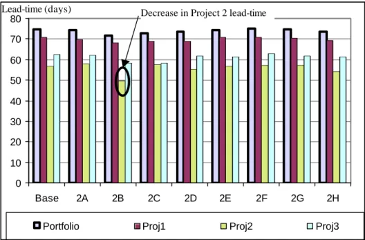
6.2.3 Effect of Adding Resources
To assess the impact of adding an extra processor of a specific type (i.e., of type A, B, or
C, etc.) on portfolio and projects’ lead times, we simulated the portfolio eight times. Each of
these eight simulations assumes that there are two processors of a certain type.12 We increase the
capacity of the processors one at a time, while keeping the capacity of the rest of the processors
at their nominal values (i.e., one processor of each type). For the processor that has a capacity of
two, when faced with a choice to work on more than one activity, it works on the one with the
highest priority and the second processor is called upon to perform work on the activity with the
second highest priority.13
12 The number of processors available for each type is entered by the user as part of the simulation inputs.
13 It is worth noting that if the processor with a capacity of two has only one activity to work on at a certain time, then having two processors available to work on the same activity does not reduce the duration of that activity. Only one processor does the work required.
Figure 10 shows the results of the eight different simulations compared to the base case
(one processor of each type). The figure shows that the addition of an extra processor (of any
type) does not really benefit the project portfolio in general (i.e., reduce mean lead-time). In this
example, at the portfolio level, no one single processor is significantly responsible for the delay
due to multi-tasking.14 Similarly, at the project level, projects 1 and 3 would not benefit from
such an increase in resources.15 However, project 2 benefits from adding a second processor of
type B (significant reduction in project 2 lead time as marked by the ellipse in the figure).
6.3 Including Switching Costs
Switching between activities typically causes a period of reduced productivity as the
processor begins the new activity. We account for this phenomenon by allowing a percentage of
the new activity’s duration to proceed at 50% efficiency. This percentage (10% for the
example)16 is converted into a number of time steps in which the reduction of the activity’s
remaining work is only reduced by half its normal amount.
Including the 10% switching penalty resulted in the distributions shown in Figure 11.
Contrary to expectation, the lead-time distribution was not shifted to the right due to switching
cost penalty. Instead, the two distributions (i.e. “without switching penalty” and “with
switching”) overlap. The reason for this is due to the fact that none of the activities were
preempted during execution and that there was a consistent priority for each activity at every
time step of the simulation. Therefore, in this graph, the magnitude of a shift can be viewed as a
measure for the amount of preemption that occurred during the execution of the projects.
14 Of course, this is only true in the case of this example problem, not for any project portfolio.
15 No statistically significant difference was detected in the means of projects 1 or 3 under the eight different resource configurations.
16
7. Summary and Conclusion
This paper discusses an extension to information flow modeling to analyze the
performance of multiple PD projects sharing a common set of development resources. We utilize
a set of activity, project, and personal attributes in order to prioritize executable activities. This
preference function is imbedded in a DSM simulation model to build lead-time distributions for
the project portfolio and the individual projects.
Some of the model limitations, which could be overcome by possible extensions, are as
follows. First, the model assumes that all the projects and their activities are known prior to
running the simulation. In some organizations, their PD portfolio evolves dynamically over time
and projects are continuously added to and deleted from the portfolio. This situation could be
accounted for by revisiting the model at whenever such an event occurs. In fact, the model could
help with the analysis of the impacts of such events. Second, projects within the same portfolio
might be interdependent through more than shared resources. That is, the success or failure of,
or rework in, one project might influence other projects. Our model assumes that projects are
only interdependent through shared resources. However, additional dependencies could also be
included. Another extension can address PD performance issues resulting from placing a ceiling
on the number of projects a processor can be involved in at any point in time. Furthermore, our
model does not currently explore overlapping of dependent activities or other alternative work
policies. However, the work policy we use could be modified. Finally, the sensitivity of
development lead time to changes in attributes’ weights could be assessed in more details by
designing a full-blown factorial experiment (where each attribute is treated as a factor) and
running the simulation for the different factor configurations [18].
In conclusion, the main advantage of the methodology presented in this paper over other
scenarios in a multi-project environment. These scenarios can include all, or a subset, of the
following: (a) feedback structure and process architecture within individual projects, (b) the use
of partitioning to arrive at an improved information flow, (c) limited resources shared among
multiple projects, (d) project switching penalties or costs, and (e) different preference profiles for
activity executions. All of the above features are implemented in a user-friendly, Excel-based
environment allowing users to interact with the simulation, adjust its parameters, and perform
References
[1] P. Adler, A. Mandelbaum, V. Nguyen, and E. Schwerer, "From Project to Process Management: Empirically-Based Framework for Analyzing Product Development Time," Management Science, Vol. 41, No. 3, pp. 458-483, March 1995.
[2] H. Bashir and V. Thomson, “Metrics for Design Projects: A Review,” Design Studies, Vol 20, No 3, pp. 263-277, May 1999.
[3] U. Belhe and A. Kusiak, “Dynamic Scheduling of Design Activities with
Resource Constraints,” IEEE Transactions on Systems, Man, and Cybernetics – Part A: Systems and Humans, Vol. 27, No. 1, January 1997, pp. 105-111.
[4] J. Brad, “Using Multicriteria Methods in Early Stages of New Product Development,” Journal of Operational Research Society, Vol. 41, No. 8, pp. 755-766, 1990.
[5] T. Browning and S. Eppinger, "A Model for Development Project Cost and Schedule Planning," M.I.T. Sloan School of Management, Cambridge, MA, Working Paper no. 4050, November 1998.
[6] P. Brucker, A. Drexl, R. Mohring and K. Neumann, “Resource Constrained Project Scheduling: Notation, Classification, Models, and Methods,” European Journal of Operational Research, Vol. 112, pp. 3-41, 1999.
[7] M. Carrascosa, S. Eppinger and D. Whitney, “Using the Design Structure
Matrix to Estimate Product Development Time,” Proceedings of the ASME Design Engineering Technical Conferences, Sep. 1998, Atlanta, Georgia, USA.
[8] R. Clemen, Making Hard Decisions: An Introduction to Decision Analysis. Duxbury Press, New York, 1996.
[9] M. Cusumano and K. Nobeoka, Thinking Beyond Lean. Free Press, 1998.
[10] S. Eppinger, D. Whitney, R. Smith and D. Gebala, "A Model-Based Method for Organizing Tasks in Product Development," Research in Engineering Design, Vol. 6, No. 1, pp. 1-13, 1994.
[11] E. Goldratt, Critical Chain. The North River Press, Great Barrington, MA., 1997.
[12] R. Keeney. Value Focused Thinking. Harvard University Press, Cambridge, MA, 1992.
[13] R. Kolisch. Project Scheduling under Resource Constraints. Physica-Verlag, 1995.
[14] A. Kumar and L. Ganesh, “Use of Petri Nets for Resource Allocation in Projects,” IEEE Transactions in Engineering Management, Vol. 45, No. 1, Feb 1998, pp. 49-56.
[15] R. Levitt, J. Thomsen, T. Christiansen, J. Kunz, Y. Jin, and C. Nass, “Simulating Project Work Processes and Organizations: Toward a Micro-Contingency Theory of Organizational Design,” Management Science, Vol. 45, No. 11, November 1999, pp. 1479-1495.
[16] M. Liberatore, “An Extension of the Analytic Hierarchy Process for Industrial R&D Project Selection and Resource Allocation,” IEEE Transactions on Engineering Management, Vol. EM-34, No. 1, pp. 12-18, Feb. 1987.
[17] M. Meyer and J. Utterback, “Product Development Time and Commercial Success,” IEEE Transactions on Engineering Management, Vol 42, No 4, pp. 297-304, Nov 1995.
[18] D. Montgomery. Design and Analysis of Experiments. New York: John Wiley & Sons, 1996.
[19] K. Neumann, Stochastic Project Networks: Temporal Analysis, Scheduling and Cost Minimization. Berlin: Springer-Verlag, 1990.
[20] D. Reinertsen. Managing the Design Factory: A Product Developer's Toolkit. Free Press, 1997.
[21] Smith, Preston and Reinertsen, Donald, Developing Products in Half the Time. New York, NY: ITP, 1995.
[22] R. Smith and J. Morrow, "Product Development Process Modeling," Design Studies, Vol. 20, pp. 237-261, 1999.
[23] G. Stalk, “Time – The Next Source of Competitive Advantage,” Harvard Business Review, Vol 66, No 4, pp. 41-51, July/Aug 1988.
[24] T. Stewart, “A Multi-Criteria Decision Support System for R&D Project Selection,” Journal of Operational Research Society, Vol. 42, No. 1, pp. 17-26, 1991.
[25] J. Warfield, "Binary Matrices in System Modeling," IEEE Transactions on Systems, Man, and Cybernetics, vol. 3, pp. 441-449, 1973.
[26] S. Wheelwright and K. Clark, "Creating Project Plans to Focus Product Development," Harvard Bus. Rev., Mar-Apr 1992.
[27] W. Winston, Operations Research: Applications and Algorithms. Wadsworth Publishing, 1997.
[28] A. Yassine, D. Falkenburg and K. Chelst, “Engineering Design Management: an
Information Structure Approach,” International Journal of Production Research, vol. 37, no. 13, 1999.
A B C D E F G H I J A A n n n B n B n n C C D D n n n E n E n F n n n n F n G n G n H n n H n I n n n I J n n J C A E J B H I D G F C C A n A n n E n E n J n n J B n n B n H n n n H I n n n I D n n D n G n n G F n n n n n F
(a) Original DSM (b) Partitioned DSM
Figure 1: DSM Example
Figure 2: DSM Representation of Three Projects and Their Aggregate DSM
Project 1 Project 2 Project 3
A1 B1 C1 D1 A2 B2 D2 A3 D3 A1 n A2 n A3 n B1 n B2 n D3 n C1 n n D2 n D1 n n Aggregate DSM 1 2 3 4 5 6 7 8 9 A1 1 n B1 2 n C1 3 n n D1 4 n n A2 5 v n B2 6 v n D2 7 v n A3 8 v v n D3 9 v v n
Activity Deadline Finished Remaining Case A t t Case B Case C
Figure 4: Schedule Pre ssure Calculation
Overall Preference
Function
Activity
Characteristics
Project
Characteristics
Personal
Characteristics
# of dependent activities Nearness to completion Rework Expectations Delay Cost Project Type Emotional factors Perceived PressureFigure 3: Attribute Hierarchy Tree
Relative Duration
0 0.2 0.4 0.6 0.8 1 Rework Risk
(a) Rework Risk
0 0.2 0.4 0.6 0.8 1 6 5 4 3 2 1 0 # Dependent Tasks
(b) Number of dependent activities
0 0.2 0.4 0.6 0.8 1 % Work Remaining (c) Nearness to completion 0 0 . 2 0 . 4 0 . 6 0 . 8 1 R e l a t i v e D u r a t i o n (d) Relative duration 0 0.2 0.4 0.6 0.8 1 60 50 40 30 20 10 0 Cost of Delay
(e) Cost of project delay
0 0.2 0.4 0.6 0.8 1 3 2 1 Project Type (f) Project type 0 0.2 0.4 0.6 0.8 1 20% 10% 0%
% Schedule Overrun (Projected)
(g) Schedule pressure 0 0.2 0.4 0.6 0.8 1 0 0.1 0.2 0.3 0.4 0.5 0.6 0.7 0.8 0.9 1 Random number Utility
(h) Personal / Random factors Figure 5: Utility Curves Used in the Simulation
Multiple DSMs
Projects/Activities
A1(t)
Active Queues
Rank Ordering
Attribute 1 Attribute 2 Attribute n
P.D. Performance
Figure 6: The Simulation Model
Schedules Activities TIME PROJECT Done No Yes Increment Simulation Clock A2(t) Aggregate DSM Partition DSM ……..
Check for unfinished activities
A1 B 1 C1 D1 E1 F1 G1 H 1 A2 B2 C2 F2 D 2 H2 B3 D 3 A3 C3 G3 H3 A1 .2 B1 .5 C1 .7 D1 .9 .4 .3 E1 F 1 .6 G1 .5 .5 H1 .9 .6 .8 .8 A2 .1 B2 .4 .4 C2 .5 F 2 .9 .7 D2 .5 .6 H2 .4 .3 .7 B3 .3 .2 .3 D3 .5 .4 A3 C3 .7 .8 G3 .8 .8 .9 H3 .8 .9
(a) Rework probabilities
A1 B 1 C1 D1 E1 F1 G1 H1 A2 B2 C2 F2 D2 H 2 B3 D3 A3 C3 G3 H3 A1 .9 B1 .5 C1 .5 D1 .9 .5 .4 E1 F1 .9 G1 .5 .4 H1 .8 .5 .8 .9 A2 .4 B2 .4 .5 C2 .5 F2 .9 .7 D2 .5 .6 H2 1.0 .6 .7 B3 .4 .4 .2 D3 .2 .6 A3 C3 .7 .5 G3 .9 .6 .5 H3 1.0 .7
(a) Rework Impacts
0 50 100 150 200 250 300 350 400 450 47 55 63 71 79 87 95 103 112 120 128 Duration (days) Frequency
(a) Lead time distributions for the overall project portfolio: with and without resource constraints
0 50 100 150 200 250 300 350 400 45 50 55 61 66 71 76 81 87 92 97 Duration (days) Frequency
(b) Lead time distributions for Project 1: with and without resource constraints
0 50 100 150 200 250 300 350 33 40 48 55 63 70 78 85 93 100 108 Duration (days) Frequency
(c) Lead time distributions for Project 2
0 100 200 300 400 500 600 700 33 44 55 66 77 88 98 109 120 Duration (days) Frequency
(d) Lead time distributions for Project 3
Figure 8: Simulation Results
0 50 100 150 200 250 300 47 55 63 71 79 87 95 103 112 120 Duration (days) Frequency
(a) Project versus Activity Attributes
0 50 100 150 200 250 300 47 55 63 71 79 87 95 103 112 120 Duration (days) Frequency
(b) Slower versus faster rework
Figure 9: Scenario Analysis
Resource Constrained No Resource Constrains Resource Constrained Project attributes only Activity attributes only Faster rework Slower rework No Resource Constrains
Figure 10: Sensitivity of Lead Time to Resource Addition
(“2A” denotes the availability of two processors of type “A” and one processor of each of the other remaining types)
0 50 100 150 200 250 300 350 47 55 63 71 79 87 95 103 112 120 128 Duration (days) Frequency
Figure 11: Including Switching Penalties
Without Switching Penalty With Switching Penalty 0 10 20 30 40 50 60 70 80 Base 2A 2B 2C 2D 2E 2F 2G 2H
Portfolio Proj1 Proj2 Proj3
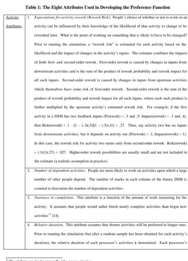
Table 1: The Eight Attributes Used in Developing the Preference Function
Activity Attributes
1. Expectations for activity rework (Rework Risk). People’s choice of whether or not to work on an activity can be influenced by their knowledge of the likelihood of that activity to change or be reworked later. What is the point of working on something that is likely to have to be changed? Prior to running the simulation, a “rework risk” is estimated for each activity based on the likelihood and the impact of changes in the activity’s inputs. The estimate combines the impacts of both first- and second-order rework. First-order rework is caused by changes in inputs from downstream activities and is the sum of the product of rework probability and rework impact for all such inputs. Second-order rework is caused by changes in inputs from upstream activities which themselves have some risk of first-order rework. Second-order rework is the sum of the product of rework probability and rework impact for all such inputs, where each such product is further multiplied by the upstream activity’s estimated rework risk. For examp le, if the first activity in a DSM has two feedback inputs (P(rework) = .3 and .5; Impact(rework) = .3 and .4), then Risk(rework) = 1 - [1 – (..3)(.3)][1 – (.5)(.4)] = .27. Then, say activity two has no inputs from downstream activities, but it depends on activity one (P(rework) = .1; Impact(rework) = 1). In this case, the rework risk for activity two stems only from second-order rework: Risk(rework) = (.1)(1)(.27) = .027. Higher-order rework possibilities are usually small and are not included in the estimate (a realistic assumption in practice).
2. Number of dependent activities. People are more likely to work on activities upon which a large number of other people depend. The number of marks in each column of the binary DSM is counted to determine the number of dependent activities.
3. Nearness to completion. This attribute is a function of the amount of work remaining for the activity. It assumes that people would rather finish nearly complete activities than begin new activities17 [14].
4. Relative duration. This attribute assumes that shorter activities will be preferred to longer ones. Prior to running the simulation (but after a random sample has been obtained for each activity’s duration), the relative duration of each processor’s activities is determined. Each processor’s
17
activities are classified as either the shortest or the longest duration activity for that processor, or else in-between. (This attribute can also be set to prefer longer activities.)
Project Attributes
5. Cost of project delay [21]. A cost of delay is supplied for each project as an input to the simulation. Activities in projects with higher costs of delay are given greater priority.
6. Project type. Project type is also given for each project as an input to the simulation. We classify project type based on project visibility and/or priority—which is either “high,” “medium/normal,” or “low.”
7. Schedule pressure. As a project falls behind schedule, pressure builds to finish its activities. Each project and each activity within it have scheduled completion times or deadlines, which are provided as inputs to the simulation. Project schedule pressure is the sum of the schedule pressure contributions of all of its activities. The schedule pressure contribution of each activit y is calculated depending on which of three cases it falls into, as shown in Figure 4. In Case A, the activity is running ahead of schedule, and it makes no contribution to its project’s schedule pressure. In Case B, the activity has not yet missed its deadline, but it is projected to do so. In this case, the schedule pressure contribution is proportional to the amount of projected overrun. In Case C, the activity has already missed its deadline. The entire, remaining portion of the activity contributes to the schedule pressure, along with the amount by which the activity is running behind its deadline. The schedule pressure contributions of all activities in a project are summed to arrive at a number, which is normalized against the deadline to arrive at a percentage of anticipated schedule overrun. As this percentage grows, schedule pressure increases. Thus, delinquent activities with early deadlines contribute much more to schedule pressure than activities with later deadlines.
Processor Attribute
8. Personal and interpersonal factors. It is impossible to represent the comprehensive set of factors that influence a processor’s choice of projects and activities. Therefore, we utilize a random factor to represent other influences, including personal and interpersonal (and even irrational) factors. The random factor can represent personality, risk propensity or averseness, interpersonal relationships—really anything not attributable to the other attributes.
Attribute Name Weight
1. Rework Expectation 0.20
2. Number of Dependencies 0.06 3. Nearness to completion 0.17
4. Relative Duration 0.07
5. Project delay cost 0.16
6. Project Type 0.16
7. Schedule pressure 0.16
8. Emotional factors 0.02
Table 2: Attribute Weights
Duration (days)
Activity
Name Min. Likely Max.
Activity Deadlines A1 5 10 15 10 B1 3 5 7 15 C1 6 7 8 22 D1 15 17 20 32 E1 6 7 8 7 F1 3 4 5 19 G1 5 7 10 29 H1 10 11 12 40 A2 5 8 10 8 B2 3 5 7 13 C2 10 13 15 26 F2 2 4 6 30 D2 8 10 14 40 H2 4 6 8 46 B3 6 7 8 7 D3 10 12 15 19 A3 8 12 15 12 C3 4 6 9 25 G3 10 10 12 35 H3 8 10 13 45
Table 3: Activity Data
Project Number
Project Type
Deadline Budget Cost of Delay ($k/day) 1 3 = Low visibility 40 80 50
2 2 = Normal 46 50 40
3 2 = Normal 45 40 50
Without Resource Constraints (Unconstrained) With Resource Constraints & Considering all Attributes Considering all Attributes & 10% Switching Penalty Mean 60.29 76.94 76.55 95% CI* 2.65 3.51 3.60 Portfolio Std. Dev. 17.62 17.71 17.22 Mean 52.86 70.79 72.17 95% CI* 0.49 10.18 0.45 Project 1 Std. Dev. 2.26 2.23 2.27 Mean 46.86 57.61 58.96 95% CI* 3.30 2.45 3.09 Project 2 Std. Dev. 15.48 11.52 14.26 Mean 54.04 64.76 63.32 95% CI* 3.16 3.04 3.97 Project 3 Std. Dev. 14.57 19.11 19.65
Table 5: Simulation Results and Comparison of Means