HAL Id: hal-01095288
https://hal.inria.fr/hal-01095288
Submitted on 13 Jan 2015HAL is a multi-disciplinary open access archive for the deposit and dissemination of sci-entific research documents, whether they are pub-lished or not. The documents may come from teaching and research institutions in France or abroad, or from public or private research centers.
L’archive ouverte pluridisciplinaire HAL, est destinée au dépôt et à la diffusion de documents scientifiques de niveau recherche, publiés ou non, émanant des établissements d’enseignement et de recherche français ou étrangers, des laboratoires publics ou privés.
Assessing the effects of architectural variations on light
partitioning within virtual wheat – pea mixtures
Romain Barillot, Abraham J. Escobar-Gutierrez, Christian Fournier, Pierre
Huynh, Didier Combes
To cite this version:
Romain Barillot, Abraham J. Escobar-Gutierrez, Christian Fournier, Pierre Huynh, Didier Combes. Assessing the effects of architectural variations on light partitioning within virtual wheat – pea mix-tures. Annals of Botany, Oxford University Press (OUP), 2014, Special Issue: Functional-Structural Plant Modelling, 114 (4), pp.13. �10.1093/aob/mcu099�. �hal-01095288�
a
Currentaddress: INRA, Centre de Versailles-Grignon, U.M.R. INRA / AgroParisTech
Type of article: original article
1
2
Title: Assessing the effects of architectural variations on light partitioning within virtual
3
wheat–pea mixtures.
4
Authornames and affiliations: Romain BARILLOT1,a,
5
Abraham J. ESCOBAR-GUTIÉRREZ2, Christian FOURNIER3,4, Pierre HUYNH1, and Didier 6
COMBES2*. 7
Addresses: 1LUNAM Université, Groupe Ecole Supérieure d'Agriculture, UPSP
8
Légumineuses, Ecophysiologie Végétale, Agroécologie, 55 rue Rabelais, BP 30748, F-49007 9
Angers cedex 01, France. 10
2
INRA, UR4 P3F, Equipe Ecophysiologie des plantes fourragères, Le Chêne - RD 150, BP 6, 11
F-86600 Lusignan, France. 12
3
INRA, UMR 759 LEPSE, F-34060 Montpellier, France 13
4
SupAgro, UMR 759 LEPSE, F-34060 Montpellier, France 14
15
Running title: Effects of plant architecture on light partitioning in wheat-pea mixtures
16
CORRESPONDING AUTHOR:didier.combes@lusignan.inra.fr
ABSTRACT
1Background and AimsPredicting light partitioning in crop mixtures is critical to improving
2
the productivity of such complex systems. Furthermore, light interception has been shown to 3
be closely linked to plant architecture.The aim of the present work was therefore to analyse 4
the relationships between plant architecture and light partitioning within wheat-pea mixtures. 5
To address this issue, we used an existing model for wheat (Fournier et al., 2003) and 6
developed a new model for pea morphogenesis. Both models were then used to assess the 7
effects of architectural variations in light partitioning. 8
MethodsFirst, a deterministic model (L-Pea) was developed in order to obtain dynamic
9
reconstructions of pea architecture. L-Pea model is based on the L-systems formalism and 10
consists of modules for „vegetative development‟ and „organ extension‟. A tripartite simulator 11
was then built up from pea and wheat models interfaced with a radiative transfer model. 12
Architectural parameters from both plant models, selected on the basis of their contribution to 13
Leaf Area Index (LAI), height and leaf geometry, were then modified in order to generate 14
contrasting architectures of wheat and pea. 15
Key resultsBy scaling-down our analysis to the organ scale, we showed that the number of
16
branches/tillers and length of internodes markedly determined the partitioning of light within 17
mixtures. Temporal relationships between light partitioning and the LAI and height of 18
different species showed that light capture is mainly related to the architectural traits involved 19
in (i) plant LAI during the early stages of development, and (ii) plant height during the onset 20
of inter-specific competition. 21
ConclusionsIn silico experiments enabled to study of the intrinsic effects of architectural
22
parameters on the partitioning of light in mixtures. Our findings showed that plant 23
architecture is an important criterion for the identification/breeding of plant ideotypes, 1
particular with respect to light partitioning. 2
3
Key words:architectural parameters, Functional Structural Plant Model, intercropping, LAI,
4
light interception, L-Systems, Pisum sativum (pea), plant architecture, plant height, Triticum 5
aestivum (wheat)
INTRODUCTION
1In the current context of improving the sustainability of agriculture, there is renewed 2
interest in the growing of crop mixtures, referred to as intercropping (Willey, 1979, Anil et al., 3
1998). Crop mixtures can indeed produce high and stabilized yields; they can also enable a 4
reduction in the use of fertilizers and pesticides and enhance biodiversity conservation (Ofori 5
and Stern, 1987, Jensen, 1996, Corre-Hellou et al., 2006, Malézieux et al., 2009). These 6
benefits result from the trade-off between the complementarity and competition between 7
mixed species with respect to resource capture and use. In particular, the ability of component 8
species in the canopy to capture light strongly determines both their potential productivity and 9
their proportion in the mixture at harvest. Understanding the modalities of light partitioning is 10
therefore a crucial area of study. 11
The partitioning of light among mixed species is closely linked to their temporal and 12
spatial development. On the one hand, the period of time where one of the crops has not yet 13
developed has important effects on the partitioning of light and hence on growth of the 14
mixture. These situations are notably encountered in relay cropping(Malézieux et al., 15
2009)wheremixed crops do not grow simultaneously but tend to exhibit a partial overlap (e.g. 16
maize-beans, groundnut-cotton). On the other hand, the interception of light by plant stands is 17
also closely related to the physical structure of the canopy (Ross, 1981a, Sinoquet and 18
Caldwell, 1995) which itself is determined by the architecture (Godin, 2000) of the 19
individuals growing within the stand (Moulia et al., 1998). Such a multi-scale description of 20
canopy structure highlights the fact that architectural parameters defined at the organ scale 21
can significantly affect light partitioning. Unlike homogeneous monospecific stands, where 22
plants have roughly the same architecture, intercropping systems involve at least two species 23
which may display differing architectural patterns (e.g. agroforestry systems, cereal–legume 24
mixtures). Characterising the architecture of intercropped plants, and its variability (genotypic 25
and environmental) is therefore a critical issue that could guide the choice of the 1
species/cultivars to be mixed in intercropping systems and hence their degree of 2
complementarity (Sinoquet and Caldwell, 1995, Sonohat et al., 2002). 3
Exploiting the variability of plant architecture is of great interest in the context of 4
intercropping systems; however, few methods are available to assess and quantify the impact 5
of different architectural patterns on the partitioning of light between mixed species. To the 6
best of our knowledge, and because of experimental and cost constraints, light partitioning 7
within interspecific mixtures cannot be assessed directly by radiation sensors (Sonohat et al., 8
2002). The only feasible alternative at present is a modelling approach that involves various 9
concepts and formalisms for (i) representation of the canopy and (ii) the calculation of light 10
interception. Most studies are based on the turbid medium approach where the canopy is 11
represented using a statistical model and light interception is given by Beer-Lambert‟s law 12
(Sinoquet et al., 1990, Monsi and Saeki, 2005). The turbid medium paradigm has thus been 13
applied to several intercropping systems such as pea–barley (Corre-Hellou et al., 2009), 14
maize-bean (Tsubo and Walker, 2002, Tsubo et al., 2005), perennial mixtures (Faurie et al., 15
1996, Lantinga et al., 1999) or agroforestry systems (Noordwijk and Lusiana, 1999). These 16
approaches were based on a simplified description of the canopy given by integrative 17
parameters such as Leaf Area Index (LAI), plant height and mean leaf inclination. However, 18
due to their underlying hypotheses, crop models coupled to the turbid medium approach 19
cannot explicitly account for plant architecture sensustricto. Therefore, such models are not 20
suitable to assess the relationships between light partitioning and architectural parameters 21
(organ scale) of the component species. Moreover, the turbid medium analogy applied to 22
intercropping systems has also been shown to produce inaccurate estimations of light 23
partitioning in some complex canopy structures (Sonohat et al., 2002, Combes et al., 2008, 24
structural plant models (FSPM), are able to take account of interactions between plant 1
architecture, their physiological functioning and environmental conditions (for a review see: 2
Fourcaud et al., 2008, Vos et al., 2010, DeJong et al., 2011). FSPMs therefore represent a 3
suitable framework to understand the modalities of light partitioning within intercropping 4
systems. Such approaches have been used to quantify light partitioning within contrasting 5
canopies: agroforestry (Lamanda et al., 2008), a legume-weed system (Cici et al., 2008) and 6
grass-legume mixtures involving perennial and annual species (Sonohat et al., 2002, Barillot 7
et al., 2011).
8
The aim of the present study was therefore to investigate the influence of architectural 9
variations on the partitioning of light among mixed species using a FSPM approach. To 10
achieve this, we decided to use grass-legume mixtures, a commonly used intercropping 11
system in temperate regions (e.g. wheat-pea, triticale-broad bean, tall fescue-alfalfa) and 12
tropical zones (e.g. maize-bean). Our approach consisted in using a wholly in silico 13
framework based on dynamic architectural models of both the species in a grass-legume 14
mixture. For the grass species, we used an existing wheat model (ADEL-Wheat, Fournier et 15
al., 2003), while for the legume species, we chose pea for which we developed a new model.
16
Both models were combined to analyse the effects of architectural changes on the level of 17
light partitioning in virtual wheat-pea mixtures. These architectural models do not account for 18
any plastic responses of plants to their environment. This approach thus enabled us to assess 19
the intrinsic effect of specific architectural traits on the partitioning of light. 20
MATERIALS AND METHODS
21Description and parameterization of the L-Pea model
22
The virtual plant model for pea (L-Pea ) was developed using the L-Py platform 23
(Boudon et al., 2012) which combines the formalism of L-systems (Lindenmayer, 1968, 24
Prusinkiewicz and Lindenmayer, 1990) with Python, an open source and dynamic 1
programming language. The structural organisation of stems was described as a modular 2
system (Godin et al., 1999) i.e. as a collection of repeated basic units called phytomers (Gray, 3
1849, White, 1979). Using this formalism, the main vegetative organs of pea were represented 4
by a bracketed string made up of the following modules: apex (apical meristem), A; 5
internodes, I; stipules, S; and axillary buds B. Thus, the apex production rule used in the L-6
Pea model is: 7
A I [S] [S][B]n A,
8
meaning that the initiation of a phytomer by the apex (A) is associated with the production 9
() of an internode (I), two stipules (S), n axillary buds (B) and an ongoing apex. Square 10
brackets are topological rules that indicate branches. Each module (virtual organ) bears its 11
own state i.e. identification (cultivar, plant, stem and phytomer to which they belong), age, 12
length and amount of intercepted light. 13
In the model proposed here, the morphogenesis of pea is dependent on the growing 14
degree day (GDD) cumulated since sowing (base temperature = 0°C). Thermal time drives the 15
two main modules represented in the L-Pea model: (i) vegetative development and (ii) the 16
extension of vegetative organs. Parameterization of the vegetative development module (Table 17
1) was derived from an experiment conducted under field conditions on pea (cv Lucy) 18
intercropped with wheat. Details on growing conditions and measurements can be found in 19
the article Barillot et al. (2014). Moreover, these data were completed by a supplementary 20
experiment designed to characterise the extension kinetics of stipules and internodes. 21
Measurements were performed on isolated pea plants grown in growth cabinets (see details in 22
[Supplementary Information]). 23
Vegetative development module 1
Rate of phytomer appearance
2
The L-Pea model does not account sensusstricto for the initiation of vegetative 3
primordia by the apical meristem (plastochron). In fact, the leaf appearance rate (RL) as
4
measured by Barillot et al. (2014) was used directly in the model to initiate the production of 5
a new phytomer which immediately starts its visible growth i.e. no hidden growth period was 6
considered. Therefore, the production and appearance of phytomers (concomitant events in 7
the model) were implemented as a linear function of the leaf appearance rate: 8
𝑁𝑝𝑦𝑡𝑜 𝑝,𝑠 (𝑡) = min(𝑅𝐿(𝑝,𝑠)∗ 𝑡, 𝑝𝑦𝑡𝑜_𝑓𝑖𝑛𝑎𝑙(𝑝,𝑠)) Equation 1
where Nphyto(p,s)(t) is the number of visible phytomers at a given thermal time t (GDD,Growing
9
Degree Day from emergence) for plant p and stem s; parameter RL(p,s)is the rate of leaf
10
appearance used as the rate of phytomer appearance (phytomer C° day-1); and phyto_final(p,s)
11
is the final number of phytomers. Parameters RL(p,s) and phyto_final(p,s) are input parameters of
12
the model which can be specified for each plant (p) and stem (s) i.e. main stems and each 13
lateral branch. Note that the phyto_final(p,s) of main stems measured in Barillot et al. (2014)
14
was low so that the model could account for death of the apical meristem of main stems, 15
which frequently occurs in winter pea cultivars that experience cold temperatures (Jeudy and 16
Munier-Jolain, 2005, Barillot et al., 2014). 17
Branching
18
Based on our previous experiment on intercropped pea (Barillot et al., 2014), we only 19
considered first-order branches. Branching is therefore handled by the model through two 20
main input parameters (Table 1) which are: (i) the number of axillary buds (nb_branchn)
21
located at each node (n) of the main stem, and (ii) the time of bud break (bud_breakrk).
22
Branches were denoted according to their topological position, i.e. main stems were denoted 23
as 0, and then branches emerging from node nof the main stem were referenced as Axis-1
n. Properly speaking, the axillary buds should rather be called “active buds” as they represent
2
those which actually lead to development of a branch and not the total number of buds. Based 3
on the measurements made by Barillot et al. (2014), the L-Pea model was set with, 4
𝑛𝑏_𝑏𝑟𝑎𝑛𝑐𝑛 = 2,0, 𝑓𝑜𝑟 1 ≤ 𝑛 ≤ 2𝑓𝑜𝑟 𝑛 > 2
Organ extension module 5
Organ growth kinetics
6
The extension of internodes and stipules is assumed to follow a β function (Yin et al., 7 2003): 8 𝐿𝑡,𝑜𝑟𝑔 = 𝐿𝑓𝑖𝑛𝑎𝑙 𝑜𝑟𝑔 1 + 𝑡𝑒𝑛𝑑𝑜𝑟𝑔 − 𝑡 𝑡𝑒𝑛𝑑𝑜𝑟𝑔 − 𝑡𝑚𝑎𝑥𝑜𝑟𝑔 𝑡 − 𝑡𝑏𝑎𝑠𝑒𝑜𝑟𝑔 𝑡𝑒𝑛𝑑𝑜𝑟𝑔 − 𝑡𝑏𝑎𝑠𝑒𝑜𝑟𝑔 𝑡𝑒𝑛𝑑 𝑜𝑟𝑔 − 𝑡𝑏𝑎𝑠𝑒 𝑜𝑟𝑔 𝑡𝑒𝑛𝑑 𝑜𝑟𝑔 − 𝑡𝑚𝑎𝑥 𝑜𝑟𝑔 , for 𝑡 < 𝑡𝑒𝑛𝑑𝑜𝑟𝑔 𝐿𝑓𝑖𝑛𝑎𝑙 𝑜𝑟𝑔 , for 𝑡 ≥ 𝑡𝑒𝑛𝑑𝑜𝑟𝑔 Equation 2
whereLfinal (mm) is the final organ length, t (°C day) the current age of the organ, tbase the
9
beginning of organ extension (°C day), tmax (°C day) the time point at which the maximum
10
rate of organ extension is reached, and tend (°C day) is the duration of organ extension. The
11
values for the parameters tbase,tmaxand tend shown in Table 1 were normalized by the time of the
12
first organ starting its extension in a phytomer. Our results showed that the development of 13
phytomers was initiated by the emergence of stipules (tbase = 0°C day) which started to grow
14
slightly earlier than internodes [Supplementary Information]. The final length reached by 15
organs (Lfinal) is defined as a function of the normalised phytomer rank ([Supplementary
16
Information]).
17 18 19
The width of stipules (Wstipule) at time twas derived from an allometric rule:
1
𝑊𝑡,𝑠𝑡𝑖𝑝𝑢𝑙𝑒 = 𝑘 ∗ 𝐿𝑡,𝑠𝑡𝑖𝑝𝑢𝑙𝑒 (R² = 0.95) Equation 3
wherek is the allometric coefficient and Lt,stipule is stipule length.
2
Senescence
3
In the L-pea model, shoot senescence only concerns stipules that are removed once 4
their lifetime has elapsed (Table 1). The values for leaf lifespan were derived from Lecoeur 5
(2005). 6
Geometric interpretation of the model 7
Internodes were associated to generalised cylinders. Stipules were reconstructed from 8
a library of about 200 geometric objects obtained from the photographs used to extract stipule 9
shape. 10
ADEL-Wheat model
11
Virtual wheat plants were obtained from a dynamic and 3D architectural model of 12
wheat development (Fournier et al., 2003). This model is available on the Openalea platform 13
(Pradal et al., 2008). The dataset was derived from an experiment carried out by Bertheloot et 14
al. (2009) where wheat (cultivar Caphorn) was grown under field conditions with low 15
nitrogen fertilization at a density of 250 plants m-2. The model simulates the elongation 16
kinetics of individual organs, and their geometric shape. The development and death of tillers 17
was also accounted for in the model and was kept constant in our simulations. 18
The input parameters of both the ADEL-Wheat and L-Pea models used to build up the virtual 19
mixtures were thus based on experiments with low nitrogen levels similar to those applied by 20
farmers in Western Europe. 21
Virtual wheat–pea mixtures: interfacing the L-Pea and ADEL-Wheat models
1
The L-pea model was implemented on the Openalea platform so that it could be 2
interfaced with ADEL-Wheat. Wheat and pea mock-ups were merged in scene graphs using 3
the PlantGL graphic library (Pradal et al., 2009). Simulations were processed from 0 to 4
2000 GDD with a time step of 50 GDD (Table 2). The inter-row spacing of mixtures was 5
0.17 m, with a final density of 125 plants m-2 for wheat and 45 plants m-2 for pea i.e. 50% of 6
the optimum density of each crop as generally encountered in Western European farming 7
practices (Corre-Hellou et al., 2006). The component species were mixed within each row in 8
virtual mixtures of 0.5x0.5 m (two rows including 18 wheat plants and 6 pea plants). 9
Light partitioning within virtual wheat–pea mixtures
10
The virtual wheat–pea mixtures were coupled with a radiative transfer model that 11
estimates the dynamics of PAR partitioning at each step of the growing cycle. Calculations of 12
light interception were provided by the nested radiosity model,Caribu, developed by Chelle 13
and Andrieu (1998). The computations only considered diffuse radiations according to the 14
Uniform OverCast (UOC) sky radiation distribution (Moon and Spencer, 1942). Diffuse 15
radiations were approximated using a set of 20 light sources. Light interception by each organ 16
was computed for each direction and then integrated over the sky vault by summing up the 17
weighted values obtained from all 20 directions. In order to prevent any border effects, the 18
basic mixture plot of 0.25 m-2 was duplicated using an option of the Caribu model. 19
Building contrasting wheat and pea architectures
20
The architectural parameters of both models were set initially to ensure the smallest 21
possible difference of LAI and height dynamics between wheat and pea. This first simulation 22
is hereinafter called the reference simulation (see detailed architecture in Table 3and Figure 23
1). 24
Architectural alterations were then applied to both plant models in order to quantify 1
their impact on light partitioning throughout the growing cycle of the mixture. These 2
architectural parameters were selected as a function of their contribution to the Leaf Area 3
Index (LAI), plant height and leaf geometry. (i) Variations in LAI were obtained by increasing 4
or decreasing the number of tillers and branches produced by wheat and pea, respectively. (ii) 5
Variations in plant height were obtained by altering the final length of internodes. (iii) During 6
previous studies (Barillot et al., 2011, Barillot et al., 2012), it was found that leaf inclination 7
had minor effects on light partitioning within virtual wheat–pea mixtures when compared to 8
the LAI and height of the species. In order to validate this assumption, light partitioning was 9
also estimated within mixtures where the leaf inclination of pea was altered. Based on the 10
initial values set for the reference simulation, 25% and 50% variations in both directions were 11
applied to each architectural parameter. 12
All simulations were performed by modifying one parameter at a time, which thus 13
represented a total of 21 simulations. The effects of each architectural parameter (simul) on 14
plant LAI and height and on light partitioning were compared to the reference simulation 15
(Ref) by calculating the relative variations: 16
𝑅𝑒𝑙𝑎𝑡𝑖𝑣𝑒 𝑣𝑎𝑟𝑖𝑎𝑡𝑖𝑜𝑛 = (𝑅𝑒𝑓 − 𝑆𝑖𝑚𝑢𝑙) 𝑅𝑒𝑓 Equation 4
17
Based on these simulations, we were able to analyse the relationships between light 18
partitioning and variations in the species ratios of LAI and height. To this end, five particular 19
stages during development were selected (see Table 2). The first dates represented the 20
vegetative stages of the two species and onset of their lateral development (branching and 21
tillering). Vertical elongation phases were then selected, as well as the flowering periods of 22
wheat and pea. The relationships between light partitioning and species LAI and height were 23
finally studied during the last stages of development nearing physiological maturity 1 (2000 GDD). 2
RESULTS
3 Reference simulation 4The dynamics of LAI, height and light interception efficiency (LIE: the fraction of 5
incident light intercepted by a species or the whole mixture) for the reference simulation are 6
shown in Figure 2. Between 200 and 2000 GDD after sowing (Figure 2A), the LAI kinetics of 7
the whole mixture and of each component species followed typical kinetics as of those 8
observed in pea–barley mixtures (e.g.Corre-Hellou et al., 2009). The mixture reached a 9
maximum LAI of 6.30 at the time of wheat and pea flowering (1400 GDD). After 1700 GDD, 10
the senescence of wheat and pea leaves gave rise to a fall in the mixture LAI to 4.45. 11
Differences between the LAI of wheat and pea did not exceed 0.66. 12
Pea was taller than wheat from the early stages of development to 1000 GDD, a period 13
which corresponds to the elongation of wheat internodes (Figure 2B). The stable height of pea 14
observed between 800 and 1000 GDD could be explained by: (i) the death of the main stem, 15
causing a cessation of vertical growth, and (ii) the delayed growth of branches that overtopped 16
the main stems as from 1100 GDD and led to a final height of 0.70 m. The height of wheat 17
also remained at 0.11 m between 400 and 700 GDD i.e. before internode elongation which 18
resulted in a maximum height of 0.70 m. 19
The LIE of the mixture increased rapidly until the final height of species had nearly 20
been reached (1500 GDD) and then stabilized at 0.9, meaning that 90% of incident light was 21
intercepted by the canopy (Figure 2C). As a consequence of these greater LAI and height 22
values, pea captured on average 62% of the light intercepted by the overall mixture up to 23
1100 GDD. The contribution of wheat to light interception by the mixture subsequently 1
averaged 57% until 1700 GDD. 2
Variations in species LAI and height in response to architectural alterations
3
LAI variations 4
Alterations in the number of branches produced by pea dramatically affected its LAI 5
from the early stages of development (400-500 GDD, Figure 3). Based on the reference 6
simulation, similar absolute variations in LAI were observed after an equivalent increase or 7
decrease in the number of branches, thus defining symmetric variations. As expected, the 8
greatest differences in LAI were observed when the number of branches increased or 9
decreased by 50% (+0.50 and -0.52, respectively). 10
Alterations in the number of tillers produced by wheat also led to strong relative 11
variations in LAI, although the amplitude was less marked than in pea (Figure 3). These 12
effects were observable from 600-650 GDD i.e. during tiller production. Maximum relative 13
variations of +0.30 and -0.37 in wheat LAI were observed at the end of tillering (850 GDD) 14
and resulted from a 50% increase or decrease in the number of tillers, respectively. Relative 15
variations in LAI then rapidly diminished as from 900 GDD under each scenario. After 16
flowering (around 1500 GDD), these plants even reached the same LAI values as those of the 17
reference simulation. This was due to a parameter relative to tiller death which led to the same 18
final number of tillers as the reference simulation because: (i) the tillers removed under the 19
-25 and -50% scenarios were also intended to regress in the reference simulation, and (ii) the 20
tillers added (+25 and +50% scenarios) were set to regress at the same time as those in the 21
reference simulation. 22
Height variations 1
Symmetrical absolute variations in the height of pea and wheat were observed after an 2
equivalent increase or decrease in internode length (Figure 4). Relative variations in pea 3
height were constant from 800 GDD to the end of the growing cycle (maximum variations of 4
0.47 and -0.47 under the +50% and -50% scenarios, respectively). 5
The effect of internode length on plant height was observed later in wheat than in pea, 6
as the elongation of wheat internodes started from 1000 GDD. Maximum relative variations 7
were observed at 1400 GDD (0.33) and 1500 GDD (-0.31) consecutive to a 50% increase or 8
decrease in internode length, respectively. 9
Effects of architectural modifications on light partitioning
10
Figure 5 shows (i) the effects of branching/tillering, internode length and leaf 11
inclination (pea) on the fraction of light (%PAR) intercepted by a particular species over the 12
interception of the whole mixture (values are thus complementary between pea and wheat), 13
and (ii) variations in %PAR expressed as a function of the reference simulation. Interestingly, 14
the modifications made to architectural parameters led to asymmetric responses of light 15
partitioning even though they symmetrically affected LAI and plant height (same absolute 16
variations observed after an increase or decrease in a given parameter). Indeed, increasing or 17
reducing the value of an architectural parameter (branching, height, or leaf inclination) did not 18
result in similar absolute variations in light partitioning but rather defined asymmetric 19
responses. 20
Branching 21
Alterations to the number of branches/tillers led to greater variations in light 22
partitioning in pea than in wheat. This was particularly the case when the number of branches 23
was reduced as this dramatically decreased the proportion of light intercepted by pea from the 24
early stages of development (500 GDD). Reducing the number of pea branches by 25% or 1
50% caused maximum losses of light interception of 17% and 53%, respectively, just before 2
the flowering stages (1250 GDD, Figure 5B). By contrast, increasing the number of branches 3
resulted in smaller variations in light partitioning than those caused by their reduction (a 20% 4
maximum gain of light capture under both the +25% and +50% scenarios). Compared to the 5
branch modifications applied to pea, the number of wheat tillers led to slight relative 6
variations in light partitioning (15% at most). The variations in wheat LAI which can be seen 7
in Figure 3 (30-35 %) therefore had little effect on light. 8
Internode length 9
Modifications to internode length (Figure 5C and D) appeared to have the most 10
dramatic effects on light partitioning when compared to branching (at most an 81% gain and a 11
65% loss in light capture). In both pea and wheat, longer internodes resulted in a marked 12
increase in light interception when compared to the reference simulation. For both species, 13
strong asymmetry was found regarding variations in light partitioning between plants 14
subjected to an increase in their internode length and in those whose internodes were reduced, 15
especially from 1500 GDD. From this stage of development, the effects of internode length 16
which had caused a gain in light interception by pea (i.e. longer internodes for pea and shorter 17
for wheat) started to decline until maturity. By contrast, alterations which increased wheat 18
height (i.e. shorter internodes for pea and longer for wheat) maintained wheat dominance in 19
terms of light interception until maturity. Figure 5D also shows that similar variations in light 20
partitioning could result from an increase in the internode length of pea, or an equivalent 21
reduction in wheat internodes. By contrast, increasing the internode length of wheat did not 22
cause a similar gain in light interception as an equivalent reduction of pea internodes. Indeed, 23
wheat was the most dominant species in terms of light capture when the internodes of pea 24
were shortened by 25% or 50% (respectively up to 76% and 85% of light captured by wheat). 25
Increasing the internode length of wheat by 50% resulted in a similar gain in light interception 1
than when the internode length of pea was reduced by 25%. 2
Leaf inclination of pea 3
Alterations to the inclination of pea leaves clearly had minor effects on light 4
partitioning when compared to the changes applied to branching and internode length. 5
Nevertheless, increasing leaf inclination by 50% (i.e. the leaves became more erect) reduced 6
light capture of pea by 18% at most. 7
Light partitioning as a function of the ratios of species LAI and height
8
The results described above evidenced the dynamics of light partitioning in response 9
to contrasting plant architectures. As illustrated in Figure 3 and Figure 4, such architectural 10
alterations induced a broad range of variations in the LAI and height of the component 11
species. The next step was therefore to analyse the relationships between light partitioning 12
and variations affecting both ratios of species LAI and height (Figure 6). This analysis was 13
performed at five particular stages of development (Table 2). 14
During the early stages of development (500 GDD), the architectural modifications 15
made mainly affected the height of pea plants (Figure 3 and Figure 4). Therefore, the ratio of 16
the species LAI (Figure 6) did not display any marked variations (except when the number of 17
pea branches was reduced by 50%). By contrast, changes to the internode length of pea led to 18
different height ratios, ranging from 1 to 1.92. Despite the reduction in its internode length, 19
pea remained the dominant species in terms of light capture, mainly due to its higher LAI 20
compared to wheat. At the end of the branching and tillering stages (850 GDD), wheat and 21
pea developed contrasting levels of LAI in response to architectural variations (the LAI ratio 22
ranged from 0.7 to 1.9). This resulted in marked variations in light partitioning as pea 23
architectural variations were applied to pea or wheat, the LAI ratios were similar, although 1
they are obviously affected in contrasting ways. Like the results observed at 500 GDD, light 2
partitioning was also linked to the height ratio, which was modified by alterations made to pea 3
internodes (wheat internodes had not started their elongation). The relationship between light 4
partitioning and the LAI ratio no longer appeared to be linear at 1000 GDD. Indeed, 5
increasing the number of branches/tillers still modified the LAI ratio but this only resulted in 6
slight variations of light partitioning. However, the sharing of light among the component 7
species was linearly related to the variations in height ratio which originated from 8
modifications to the internode length of pea. Under these scenarios, light intercepted by pea 9
ranged from 28% to 69% of the total light interception. At flowering (1500 GDD), the onset 10
of internode elongation in wheat generated contrasting vertical dominance (the height ratio 11
ranged from 0.63 to 1.20) which markedly affected light partitioning (between 15% and 70% 12
of light captured by pea). Figure 6 also shows that alterations to internode length at 1500 and 13
2000 GDD led to similar absolute variations in height ratio and light partitioning, whether 14
they were made to pea or wheat. The effect of the LAI ratio on light partitioning continued to 15
decline at maturity (2000 GDD). The LAI ratio ranged from 0.48 to 1.45 but only increased 16
the light interception of pea by 10%. Variations in the height ratio at this stage of development 17
were similar to those observed at 1500 GDD. However, the link with light partitioning 18
appeared to become non-linear, particular with the most marked alterations to internode 19
length (±50%). 20
DISCUSSION
21The L-Pea model: a deterministic approach to modelling the aerial morphogenesis of
22
pea
23
For the purposes of our study, we developed a deterministic model that generate a 24
simplified and dynamic representation of pea architecture. Pea morphogenesis was modelled 25
as a function of thermal time, in line with the work by Turc and Lecoeur (1997) who found 1
stable linear relationships between thermal time and the number of expanded leaves in pea 2
whatever the plant growth rate, cultivar and period of the cycle. As mentioned by 3
Prusinkiewicz (1998), the design of developmental models necessitates the definition of rules 4
to describe the emergence of new modules during development as well as the growth kinetics 5
of modules produced previously. During the present study, these rules were considered in light 6
of the results of two separate experiments, one conducted under field conditions (Barillot et 7
al., 2014) and the other in a growth cabinet. The latter measurements, dedicated to
8
characterising stipules and internode elongation, were obtained on pea plants which had not 9
been grown in a mixture with wheat. These kinetics were not therefore intended to accurately 10
quantify the extension of pea internodes and stipules in an intercropping system, but rather to 11
capture the main characteristics of their extension and coordination. Furthermore, the kinetics 12
of organ extension were likely to have a limited influence on our results as we performed an 13
analysis of the sensitivity of light partitioning to alterations in the number of branches/tillers 14
and internode length. 15
Moreover, the L-Pea model was used to represent realistic/measured architectures of 16
pea plants (resulting from the integration of environmental effects) but was not designed to 17
reproduce the responses of plants to the environment. Indeed, the current version of the L-Pea 18
model does not account for environmental influences on pea morphogenesis (e.g. intra/inter-19
specific competition, abiotic or biotic factors). Although this goes beyond the scope of this 20
paper, future studies on the L-Pea model could be performed in order to develop a more 21
mechanistic approach to pea development that might include feedback between the resource 22
status of plants and their morphogenesis. 23
An in silico experiment to assess the effects of contrasting architectures on light
1
partitioning within mixtures
2
An ability to manipulate light partitioning in multi-specific stands is crucial to 3
managing the balance between component species and also determining the final yield of the 4
mixture (Ofori and Stern, 1987, Keating and Carberry, 1993, Sinoquet and Caldwell, 1995, 5
Malézieux et al., 2009, Louarn et al., 2010). The present work therefore focused on the 6
architectural determinants (i.e. physical modalities) of light partitioning in intercropping 7
systems, but did not aim to study competition for this resource. As a first step towards 8
understanding competition for light within intercropping systems, in silico experiments were 9
performed using two deterministic FSPMs of wheat and pea morphogenesis, without taking 10
any account of the plastic responses of plants to their environment. The tripartite simulator 11
(wheat-pea-light) built up for this study therefore represented a heuristic tool to assess the 12
intrinsic effects of individual architectural parameters. More generally, this simulator could be 13
used to test hypotheses that are inaccessible to “conventional” experiments because of 14
technical or time constraints. Although the environmental responses of plants were not taken 15
into account, the contrasting architectures of plants that were generated during this work 16
could mimic the situations encountered in different intercropping systems subject to particular 17
environmental conditions (e.g. agroforestry systems where one species largely overtops 18
another). 19
By scaling-down our analysis to the organ scale, this study provided novel information 20
on the temporal sensitivity of light partitioning to the architecture of component species. 21
Some previous works had also aimed to analyse the relationships between light partitioning 22
and the simplified or explicit architecture of component species (Sinoquet and Caldwell, 23
1995, Louarn et al., 2012). However, these studies focused on integrative parameters (height, 24
LAI) which could not discriminate the effects of explicit architectural parameters defined at 25
the organ scale. As reported by several studies (Sinoquet and Caldwell, 1995, Barillot et al., 1
2011, Barillot et al., 2012, Louarn et al., 2012), the present results further confirmed that light 2
partitioning is strongly related to the ratio of the component species LAI and height. However, 3
this relationship appeared to be dependent on the species considered and was not constant 4
throughout the growing cycle. Light partitioning during the early stages of development was 5
closely linked to the contribution of each component species to the LAI of the mixture. 6
Species with high capacity for branching therefore displayed marked competitiveness for light 7
capture. As the mixture grew, the interception of each plant started to be altered by its 8
neighbours (e.g. foliage clumping, mutual shading) and inter-specific competition [for light] 9
thus started to modify the relative importance of architectural parameters. When species 10
started their vertical growth (internode elongation), the relationship between light partitioning 11
and the ratio of the component species LAI was no longer linear. During later stages of the 12
growing cycle, light partitioning tended to be related to height ratio. These results were 13
consistent with a previous study carried out on virtual wheat–pea mixtures derived from the 14
digitization of several pea cultivars grown under greenhouse conditions (Barillot et al., 2012). 15
The present work, based on dynamic models of both wheat and pea has therefore provided 16
new information on the temporal variations of light partitioning throughout the growing cycle 17
of the two species. Furthermore, the use of architectural models enabled us to assess the 18
effects of specific parameters with respect to both wheat and pea architectures. 19
Leaf inclination also affected light partitioning but to a lesser extent than alterations to 20
branching or internode length. This architectural trait does not appear to be a factor that 21
should be targeted as a priority when manipulating the partitioning of light within mixtures. 22
Nevertheless, Sarlikiotiet al. (2011) reported that the leaf inclination of tomato impacted the 23
distribution of light interception rather than total light interception. Further, the effect of leaf 24
significantly improve the light interception of plants that are already the tallest in the mixture 1
(see for example the alfalfa-tall fescue mixtures described by Barillot et al., 2011). In our 2
simulations based on wheat-pea mixtures, light partitioning was found to be highly sensitive 3
to the number of tillers/branches and to internode length. Although they were significant, the 4
effects of wheat internode length on light capture were less marked than in pea. Ciciet al. 5
(2008) also reported that in chickpea, changes to internode length did not lead to the strongest 6
competition with sow thistle when compared to phyllochron variations, for example. By 7
contrast, Lemerleet al. (2001) suggested that wheat plants with longer internodes had an 8
enhanced competitive ability for light capture versus weeds. It therefore appears that an 9
assessment of the effects of a given architectural parameter (e.g. branching, internode length 10
or leaf inclination) on light partitioning should be carried out with respect to both: (i) the 11
whole plant structure (i.e. other architectural parameters), and (ii) the morphogenesis of the 12
neighbouring plant/species. Indeed, the determinant parameters that are known to affect light 13
interception in pure stands (e.g. number of tillers or internode length) do not necessarily have 14
the same quantitative effects in multi-specific stands, depending on the behaviour of the 15
component species. Moreover, modifications made to branching and internode length 16
triggered asymmetric variations in light partitioning, which means that: (i) other ranges of 17
variation in architectural parameters should be tested in order to better explore the responses 18
of light partitioning, and (ii) interactions with other parameters need to be taken into account 19
e.g. leaf area distribution and clumping (Ross, 1981b, Lantinga et al., 1999).
20
CONCLUSION
21The questions addressed in this paper necessitated the development of a 3D and 22
dynamic architectural model of pea (L-Pea) which, to our knowledge, is the first pea model to 23
have become available in the literature. The L-Pea model is based on a deterministic approach 24
that enabled the generation of simplified representations of pea architecture. Although they 25
may go beyond the scope of the present paper, further studies should be performed in order to 1
obtain a more mechanistic approach to the modelling of pea morphogenesis. For instance, 2
mechanistic rules could be implemented for branching, a process which is known to be 3
closely dependent on genotype (Arumingtyas et al., 1992, Barillot et al., 2012) and 4
environmental factors such as low temperatures (Jeudy and Munier-Jolain, 2005) and plant 5
density (Spies et al., 2010) and include the effects of light quality (Casal et al., 1986, Ballaré 6
and Casal, 2000). Integrating such responses in a model would nevertheless require the 7
conduct of further studies in order to enhance our understanding of the regulation of 8
branching and in particular how internal factors (e.g. hormone balance) respond to 9
environmental signals (Evers et al., 2011). 10
During the present study, the L-Pea model was used within a complex modelling 11
framework that integrated an architectural model of wheat as well as a light model. Such 12
virtual environments can facilitate approaches designed to define plant ideotypes adapted to 13
intercropping by targeting morphological traits that need to be integrated in breeding 14
programmes. Indeed, scaling the analysis at the organ level can facilitate links with geneticists 15
and breeders. Taking the example of wheat–pea mixtures, several genes that govern pea 16
architecture (branching, height, leaf-type) have already been identified (e.g. for pea, 17
Arumingtyas et al., 1992, Kusnadi et al., 1992, Huyghe, 1998). For wheat (and other cereals), 18
the studies performed during the green revolution also enabled the control of plant height 19
(Evenson, 2003), notably by introducing dwarf genes (Hedden, 2003). Our study also 20
highlighted the importance of considering plant architecture in the choice of the 21
species/genotypes used for intercropping systems. Thus alongside standard criteria such as 22
crop earliness, disease sensitivity and yield, attention should also be paid to the architectural 23
traits involved in LAI and plant height. In particular, we showed that both branches and 24
species to compete for light. Integration of these architectural traits should also take account 1
of the fact that their impact on light partitioning will vary during the growing cycle, thus 2
requiring greater better knowledge of the dynamic aspects of plant morphogenesis. 3
LITERATURE CITED
4Anil, Park, Phipps, Miller.1998. Temperate intercropping of cereals for forage: a review of
5
the potential for growth and utilization with particular reference to the UK. Grass & 6
Forage Science,53: 301-317.
7
Arumingtyas EL, Floyd RS, Gregory MJ, Murfet IC.1992. Branching in Pisum:
8
inheritance and allelism tests with 17 ramosusmutants. Pisum Genetics,24: 17-31. 9
Ballaré CL, Casal JJ.2000. Light signals perceived by crop and weed plants. Field Crops
10
Research,67: 149-160.
11
Barillot R, Combes D, Chevalier V, Fournier C, Escobar-Gutiérrez AJ.2012. How does
12
pea architecture influence light sharing in virtual wheat-pea mixtures? A simulation 13
study based on pea genotypes with contrasting architectures.AoB Plants,pls038. 14
Barillot R, Combes D, Pineau S, Huynh P, Escobar-Gutiérrez AJ. 2014. Comparison of
15
the morphogenesis of three genotypes of pea (Pisum sativum) grown in pure stands 16
and wheat-based intercrops. AoB Plants, 6. 17
Barillot R, Louarn G, Escobar-Gutiérrez AJ, Huynh P, Combes D.2011. How good is the
18
turbid medium-based approach for accounting for light partitioning in contrasted 19
grass-legume intercropping systems? Annals of Botany,108: 1013-1024. 20
Bertheloot J, Andrieu B, Fournier C, Martre P. 2009. Modelling Nitrogen Distribution in
21
Virtual Plants, as Exemplified by Wheat Culm During Grain Filling. . Proceedings of 22
the 2009 Plant Growth Modeling, Simulation, Visualization, and Applications.Beijing,
23
China, IEEE Computer Society. 24
Boudon F, Pradal C, Cokelaer T, Prusinkiewicz P, Godin C.2012. L-Py: an L-System
25
simulation framework for modeling plant development based on a dynamic language. 26
Frontiers in Plant Science,3.
27
Casal JJ, Sanchez RA, Deregibus VA.1986. The effect of plant density on tillering: The
28
involvement of R/FR ratio and the proportion of radiation intercepted per plant. 29
Environmental and Experimental Botany,26: 365-371.
30
Chelle M, Andrieu B.1998. The nested radiosity model for the distribution of light within
31
plant canopies.Ecological Modelling,111: 75-91. 32
Cici SZ-H, Adkins S, Hanan J.2008. A Canopy Architectural Model to Study the
33
Competitive Ability of Chickpea with Sowthistle.Annals of Botany,101: 1311-1318. 34
Combes D, Chelle M, Sinoquet H, Varlet-Grancher C.2008. Evaluation of a turbid medium
35
model to simulate light interception by walnut trees (hybrid NG38 x RA and 36
Juglansregia) and sorghum canopies (Sorghum bicolor) at three spatial
37
scales.Functional Plant Biology,35: 823-836. 38
Corre-Hellou G, Faure M, Launay M, Brisson N, Crozat Y.2009. Adaptation of the STICS
39
intercrop model to simulate crop growth and N accumulation in pea–barley intercrops. 40
Field Crops Research,113: 72-81.
41
Corre-Hellou G, Fustec J, Crozat Y.2006. Interspecific competition for soil N and its
42
interaction with N2 fixation, leaf expansion and crop growth in pea–barley intercrops.
43
Plant and Soil,282: 195-208.
DeJong TM, Da Silva D, Vos J, Escobar-Gutiérrez AJ.2011. Using functional–structural
1
plant models to study, understand and integrate plant development and ecophysiology. 2
Annals Of Botany,108: 987-989.
3
Evenson RE.2003. Assessing the Impact of the Green Revolution, 1960 to 2000. Science,300:
4
758-762. 5
Evers JB, van der Krol AR, Vos J, Struik PC.2011. Understanding shoot branching by
6
modelling form and function. Trends in Plant Science,16: 464-467. 7
Faurie O, Soussana JF, Sinoquet H.1996. Radiation interception, partitioning and use in
8
grass -clover mixtures. Annals of Botany,77: 35-46. 9
Fourcaud T, Zhang X, Stokes A, Lambers H, Körner C.2008. Plant Growth Modelling and
10
Applications: The Increasing Importance of Plant Architecture in Growth Models. 11
Annals of Botany,101: 1053-1063.
12
Fournier C, Andrieu B, Ljutovac S, Saint-Jean S.2003.ADEL-wheat: A 3D architectural
13
model of wheat development. Proceedings of the 2003 Plant Growth Modeling, 14
Simulation, Visualization, and Applications.Beijing, China, IEEE Computer Society,
15
54-63. 16
Godin C.2000. Representing and encoding plant architecture: A review. Annals of Forest
17
Science,57: 413-438.
18
Godin C, Costes E, Sinoquet H.1999. A method for describing plant architecture which
19
integrates topology and geometry.Annals Of Botany,84: 343-357. 20
Gray A. 1849. On the composition of the plant by phytons, and some applications of
21
phyllotaxis.Proceedings of the American Association for the Advancement of Science. 22
Hedden P.2003.The genes of the Green Revolution.Trends in Genetics,19: 5-9.
23
Huyghe C.1998. Genetics and genetic modifications of plant architecture in grain legumes: a
24
review. Agronomie,18: 383-411. 25
Jensen ES.1996. Grain yield, symbiotic N2 fixation and interspecific competition for
26
inorganic N in pea-barley intercrops. Plant and Soil,182: 25-38. 27
Jeudy C, Munier-Jolain N.2005.Developpement des ramifications. In: Munier-Jolain N,
28
Biarnes V, Chaillet I, Lecoeur J, Jeuffroy M-H eds. Agrophysiologie du pois 29
protéagineux. Paris, Inra-Quae, 51-58.
30
Keating BA, Carberry PS.1993. Resource capture and use in intercropping: solar radiation.
31
Field Crops Research,34: 273-301.
32
Kusnadi J, Gregory M, Murfet IC, Ross JJ, Bourne F.1992. Internode length in Pisum:
33
phenotypic characterisation and genetic identity of the short internode mutant 34
Wt11242. Pisum Genetics,24: 64-74. 35
Lamanda N, Dauzat J, Jourdan C, Martin P, Malézieux E.2008. Using 3D architectural
36
models to assess light availability and root bulkiness in coconut agroforestry systems. 37
Agroforestry Systems,72: 63-74.
38
Lantinga EA, Nassiri M, Kropff MJ.1999. Modelling and measuring vertical light
39
absorption within grass-clover mixtures. Agricultural and Forest Meteorology,96: 71-40
83. 41
Lecoeur J.2005.Developpementvegetatif.In: Munier-Jolain N, Biarnes V, Chaillet I, Lecoeur
42
J, Jeuffroy M-H eds. Agrophysiologie du pois protéagineux. Paris, Inra-Quae, 27-45. 43
Lemerle D, Gill GS, Murphy CE, Walker SR, Cousens RD, Mokhtari S, Peltzer SJ,
44
Coleman R, Luckett DJ.2001. Genetic improvement and agronomy for enhanced
45
wheat competitiveness with weeds. Australian Journal of Agricultural Research,52: 46
527-548. 47
Lindenmayer A.1968. Mathematical models for cellular interactions in development I.
48
Filaments with one-sided inputs. Journal of Theoretical Biology,18: 280-299. 49
Louarn G, Corre-Hellou G, Fustec J, Lô-Pelzer E, Julier B, Litrico I, Hinsinger P,
1
Lecomte C.2010. Déterminants écologiques et physiologiques de la productivité et de
2
la stabilité des associations graminées-légumineuses. Innovations Agronomiques,11: 3
79-99. 4
Louarn G, Da Silva D, Godin C, Combes D.2012. Simple envelope-based reconstruction
5
methods can infer light partitioning among individual plants in sparse and dense 6
herbaceous canopies. Agricultural and Forest Meteorology,166–167: 98-112. 7
Malézieux E, Crozat Y, Dupraz C, Laurans M, Makowski D, Ozier-Lafontaine H,
8
Rapidel B, de Tourdonnet S, Valantin-Morison M.2009. Mixing plant species in
9
cropping systems: concepts, tools and models.A review.Agron. Sustain. Dev.,29: 43-10
62. 11
Monsi M, Saeki T.2005. On the Factor Light in Plant Communities and its Importance for
12
Matter Production.Annals Of Botany,95: 549-567. 13
Moon P, Spencer DE.1942. Illumination from a non-uniform sky. Illuminating Engineering
14
Society 37: 707-726.
15
Moulia B, Edelin C, Jeuffroy MH, Allirand JM, Loup C, Chartier M.1998.Premiers
16
éléments d'analyse du développement architectural des herbacées cultivées. In: 17
Maillard P, Bonhomme R eds. Fonctionnement des peuplements végétaux sous 18
contraintes environnementales. Paris, France, INRA editions, 149-184.
19
Noordwijk M, Lusiana B.1999.WaNuLCAS, a model of water, nutrient and light capture in
20
agroforestry systems. In: Auclair D, Dupraz C eds. Agroforestry for Sustainable Land-21
Use Fundamental Research and Modelling with Emphasis on Temperate and
22
Mediterranean Applications. Springer Netherlands, 217-242.
23
Ofori F, Stern WR.1987. Cereal-legume intercropping systems. Advances in agronomy,41:
24
41-90. 25
Pradal C, Boudon F, Nouguier C, Chopard J, Godin C.2009. PlantGL: A Python-based
26
geometric library for 3D plant modelling at different scales. Graphical Models,71: 1-27
21. 28
Pradal C, Dufour-Kowalski S, Boudon F, Fournier C, Godin C.2008. OpenAlea: a visual
29
programming and component-based software platform for plant modelling. Functional 30
Plant Biology,35: 751-760.
31
Prusinkiewicz P.1998.Modeling of spatial structure and development of plants: a
32
review.ScientiaHorticulturae,74: 113-149. 33
Prusinkiewicz P, Lindenmayer A.1990. The algorithmic beauty of plants, New-York,
34
Springer-Verlag. 35
Ross J.1981a. Role of phytometric investigations in the studies of plant stand architecture and
36
radiation regime. In: Ross J ed. The radiation regime and architecture of plant 37
stands.The Hague, The Netherlands, Junk, W., 9-11.
38
Ross J.1981b.Spatial distribution of phytoelements in stands. In: Ross J ed. The radiation
39
regime and architecture of plant stands.The Hague, The Netherlands, Junk, W., 66-89.
40
Sarlikioti V, de Visser PHB, Marcelis LFM.2011. Exploring the spatial distribution of light
41
interception and photosynthesis of canopies by means of a functional-structural plant 42
model. Annals Of Botany,107: 875-883. 43
Sinoquet H, Caldwell MM.1995.Estimation of light capture and partitioning in intercropping
44
systems. In: Sinoquet H, Cruz P eds. Ecophysiology of tropical intercropping. Paris, 45
INRA Editions, 79-97. 46
Sinoquet H, Moulia B, Gastal F, Bonhomme R, Varlet -Grancher C.1990. Modeling the
47
radiative balance of the components of a well-mixed canopy: application to a white 48
clover-tall fescue mixture.ActaOecologica-International Journal of Ecology,11: 469-49
486. 50
Sonohat G, Sinoquet H, Varlet-Grancher C, Rakocevic M, Jacquet A, Simon JC, Adam
1
B.2002. Leaf dispersion and light partitioning in three-dimensionally digitized tall
2
fescue-white clover mixtures.Plant, Cell and Environment,25: 529-538. 3
Spies JM, Warkentin T, Shirtliffe S.2010. Basal branching in field pea cultivars and
yield-4
density relationships.Canadian Journal of Plant Science,90: 679-690. 5
Tsubo M, Walker S.2002. A model of radiation interception and use by a maize-bean
6
intercrop canopy. Agricultural and Forest Meteorology,110: 203-215. 7
Tsubo M, Walker S, Ogindo HO.2005. A simulation model of cereal-legume intercropping
8
systems for semi-arid regions: I. Model development. Field Crops Research,93: 10-22. 9
Turc O, Lecoeur J.1997. Leaf Primordium Initiation and Expanded Leaf Production are
Co-10
ordinated through Similar Response to Air Temperature in Pea (Pisum sativum L.). 11
Annals of Botany,80: 265-273.
12
Vos J, Evers JB, Buck-Sorlin GH, Andrieu B, Chelle M, de Visser PHB.2010.
Functional-13
structural plant modelling: a new versatile tool in crop science. Journal of 14
Experimental Botany,61: 2101-2115.
15
White J.1979. The Plant as a Metapopulation.Annual Review of Ecology and Systematics,10:
16
109-145. 17
Willey RW.1979. Intercropping-its importance and research needs. Part 1.Competition and
18
yield advantages.Field Crop Abstracts,32: 1-10. 19
Yin X, Goudriaan J, Lantinga EA, Vos J, Spiertz HJ.2003. A Flexible Sigmoid Function of
20
Determinate Growth. Annals of Botany,91: 361-371. 21
FIGURES
1Figure 1: Vertical profile of the final length of the wheat and pea internodes used in the 2
reference simulation. The internode length of wheat is specified for the main stem (MS) and 3
four tillers (T1 to T4). 4
Figure 2: Dynamics of LAI (A), plant height (B) and Light Interception Efficiency (LIE, C) in 5
the reference simulation as a function of thermal time. These dynamics are shown for both the 6
overall mixture and the component species (pea and wheat). 7
Figure 3: Relative variations in the LAI of pea (upper panel) and wheat (lower panel) 8
estimated from the reference simulation. Variations were obtained by modifying the number 9
of branches or tillers. The colour gradient indicates the amplitude of the modifications applied 10
to the architectural parameters. 11
Figure 4: Relative variations in the height of pea (upper panel) and wheat (lower panel) 12
estimated from the reference simulation. Variations were obtained by modifying the final 13
length of internodes. The colour gradient indicates the amplitude of the modifications applied 14
to the architectural parameters. 15
Figure 5: Dynamics (left) and relative variations (right, estimated from the reference 16
simulation, in straight lines) of light partitioning (%PAR). %PAR is expressed as the fraction 17
of light intercepted by a species (left and right axis for pea and wheat, respectively) over the 18
total interception of the mixture. Therefore, %PAR values are complementary between pea 19
and wheat and those of relative variations are the opposite. The number of branches, internode 20
length and leaf inclination (for pea only) were altered for both pea (circles) and wheat 21
(triangles) following the colour gradient. 22
Figure 6: Relationship between light partitioning (%PAR, ratio of light intercepted by one 1
species to the overall interception of the mixture) and the species ratios of LAI (left) and 2
height (right) at five particular stages of development. Variations in the ratios of LAI and 3
height resulted from architectural alterations applied to pea (circles) and wheat (triangles) 4
following the colour gradient. 5
TABLES
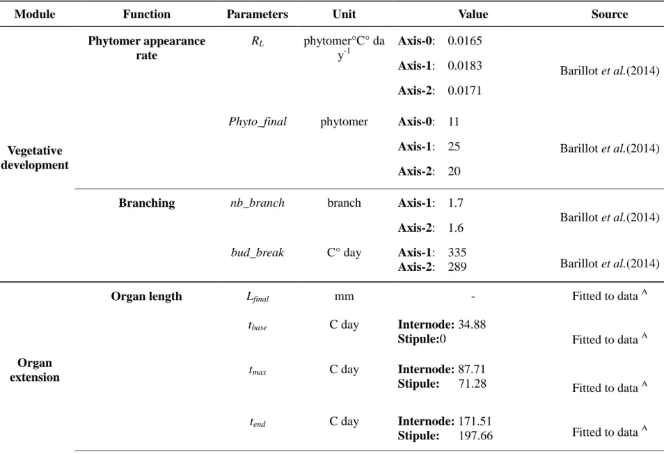
1Table 1: Parameters of L-Pea model. Main stems are denoted as Axis-0 and branches are distinguished according to their nodal position on the main stem. Axis-1: branches developing at the first node; Axis-2: second node.
Module Function Parameters Unit Value Source
Vegetative development Phytomer appearance rate RL phytomer°C° da y-1 Axis-0: 0.0165 Axis-1: 0.0183 Axis-2: 0.0171 Barillot et al.(2014)
Phyto_final phytomer Axis-0: 11 Axis-1: 25 Axis-2: 20
Barillot et al.(2014)
Branching nb_branch branch Axis-1: 1.7
Axis-2: 1.6 Barillot et al.(2014)
bud_break C° day Axis-1: 335
Axis-2: 289 Barillot et al.(2014)
Organ extension
Organ length Lfinal mm - Fitted to data A
tbase C day Internode: 34.88
Stipule:0 Fitted to data A
tmax C day Internode: 87.71
Stipule: 71.28 Fitted to data A
tend C day Internode: 171.51
Allometric coefficient k dimensionless 0.57 Fitted to data A
Senescence lifespan C day 480 Adapted from
Lecoeur (2005)
A
See experiment described in Supplementary Information
1
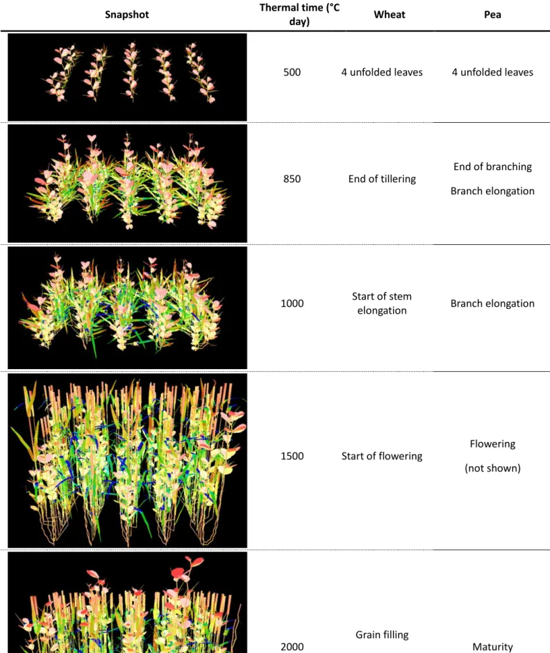
Table 2: Specific stages of the development of wheat and pea illustrated by side views of the virtual mixtures. The colour gradient is a function of the light intercepted by different organs (from blue to red).
Snapshot Thermal time (°C
day) Wheat Pea
500 4 unfolded leaves 4 unfolded leaves
850 End of tillering End of branching Branch elongation
1000 Start of stem
elongation Branch elongation
1500 Start of flowering Flowering (not shown)
2000
Grain filling
1
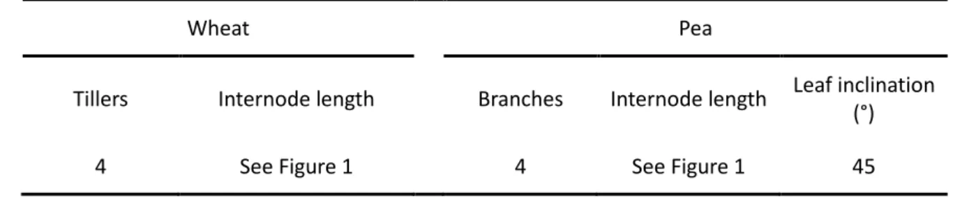
Table 3: Input parameters of the ADEL-Wheat and L-Pea models as used for the reference simulation
Wheat Pea
Tillers Internode length Branches Internode length Leaf inclination (°)