Development of a steam generating dynamometer for gas powered turboshaft engines by Edward Higb Igbubebe.

Development of a Steam Generating Dynamometer

for Gas Powered Turboshaft Engines

by

Edward John Ognibene

B.E.M.E., SUNY at Stony Brook (1989)

M.S.M.E., Massachusetts Institute of Technology (1991)

Submitted to the Department of Mechanical

Engineering in partial fulfillment of the

requirements for the degree of

DOCTOR OF PHILOSOPHY

at the

MASSACHUSETTS INSTITUTE of TECHNOLOGY

May 1995

© Massachusetts Institute of Technology, 1995 All rights reserved

Signature of Author

Certified by

Deparm~ rof Mec cal Engineering

M~' May22, 1995

4v -/ /- ' I Ho - - - '

-Professor Joseph(L. Smith, Jr. Thesis Supervisor

Accepted by

IMASSACHUSETTS INSTITUTE OF TECHtOLOGY

" ""-"ProS ssor Ain A. Sonin Chairman, Graduate Committee Department of Mechanical Engineering

-Development of a Steam Generating Dynamometer

for Gas Powered Turboshaft Engines

by Edward John Ognibene B.E.M.E., SUNY at Stony Brook (1989)

M.S.M.E., Massachusetts Institute of Technology (1991) Submitted to the Department of Mechanical

Engineering in partial fulfillment of the requirements for the degree of DOCTOR OF PHILOSOPHY

Abstract

Many types of dynamometers are available that operate according to various physical

principles, ranging from cavitation to incidence or shock. Some examples are, electric

eddy-current generators, perforated disc evaporators, and Froude type water brakes. However, these machines generally suffer from low-power-density, short mechanical life, or a small performance envelope.

To overcome these problems a new type of hydraulic dynamometer has been developed that

operates by generating an organized high-speed free-surface liquid flow that helically

recirculates on the inside surface of a torus. The liquid is accelerated by a rotor to a speed at which shaft-power input is absorbed by primarily frictional dissipation in the liquid. Power absorption (P) is a function of both rotor speed (co) and liquid level in the working compartment. As power is absorbed a portion of the recirculating liquid is vaporized.

There is a large radial pressure gradient across the liquid sheet due to streamline curvature that confines boiling to a thin layer near the free surface. Furthermore, phase separation

occurs, resulting in the evolution of a vapor core surrounded by a liquid sheet. This is a

significant design advantage because nearly pure vapor can be vented (to atmosphere) by

tapping into the core region. This minimizes feed-water requirements and eliminates the need for bulky support apparatus. These features result in a portable, high-power-density dynamometer, with a long-life and wide operational envelope.

A rigorous method is presented for the design of these new dynamometers based on a flow

model, blading algorithm, numerical programs, and empirical data. The numerical

programs are useful for predicting P as a function of w and liquid level, investigating the effect of parameter variations, and making off-design performance estimates. Furthermore, scaling laws are presented that are useful for making rough performance extrapolations. For example, P scales with size (D) to the fifth power.

To substantiate predictions, a blade cascade experiment and a low-speed prototype were

developed and tested. The results confirmed theories about the basic nature of the flow and verified the blading algorithm. Finally, control scenarios are presented that aid in the

application of this new dynamometer.

Thesis Supervisor: Dr. Joseph L. Smith, Jr. Title: Professor of Mechanical Engineering

Acknowledgments

I would like to thank many people for their support during my doctoral experience at MIT. First, I am particularly grateful to Professor Joseph Smith for his unending enthusiasm and motivation throughout my experience here. His extremely broad engineering knowledge base and keen physical intuition continues to astonish me, and I am very fortunate to have had the opportunity to work with him. I would also like to thank my other Thesis

Committee members Professor A. Douglas Carmichael and Doctor Choon S. Tan for their invaluable advice, and encouragement, for which I am very grateful.

I would also like to thank the people in the graduate office, especially Leslie Regan, for helping to make my experience at MIT as pleasurable as possible. She was always very helpful, and often did much more then she was required to. The department is fortunate to have such a devoted and capable person. I am also very grateful to Lisa Desautels and Doris Elsemiller, in the Cryo Lab, for all their help and assistance.

There are many graduate students that I would like to thank, particularly Gregory Nellis, for his help with the data acquisition system, for reviewing this thesis, and for his

comradery. I also want to thank Sankar Sunder, Bill Grassmyer, Hayong Yun, Hua Lang, Mac Whale, and Chris Malone, for their helpful inputs and support during those endless lab days. I would also like to thank Mike Demaree, and Bob Gertsen, for their technical support during the experimental phase of the project.

I also want to thank my family, particularly my mother and father, for all their help and support throughout my experience at MIT. Strong family ties make it easy to persevere, and help keep things in perspective. I am especially grateful to my wife, Donna, for her love, encouragement, and motivation to continue on. I realize and appreciate the sacrifices she made to make this thesis possible.

Finally, I wish to acknowledge the financial support of Textron-Lycoming, which funded a significant portion of this work. Specifically, I would like to thank John Twarog and Richard Lambert for their continued enthusiasm and interest in the project.

Table of Contents

A bstract . . . .. . ... 2

Dedication .

... 3

Acknowledgments ... 4

Table of Co

ntents

...

...

5

List of Figures ...

7

Nomenclature ...

9

1 Conceptualization of Recirculating Flow Steam Generating Dynamometer

1.1 Background ...

...

... 10

1.2 New Dynamometer Concept ... 12

1.3 Resulting Advantage . s ... 16

1.4 Outline of Thesis

...

17

2 Investigation of Power Absorbing Mechanisms 2.1 Overview ... 19

2.2 Hydraulic Jump Induced Dissipation ... 19

2.3 Shear Stress Induced Dissipation .

...

2...

29

3 Development of Dynamometer Flow Model 3.1 Basic Flow Model ... 32

3.2 Power Balance Between Rotor Input and Recirculating Fluid ... 34

3.3 Friction Factor Prediction & the Effect of Streamline Curvature ... 36

4 Blade Generation Algorithms & Programs 4.1 Overview . ... 38

4.2 Base Curve Development ... 39

4.3 Inner Curve Development... 43

5 Flow Visualization Experiment .. Linear Blade Cascades

5.1 Objectives and Overview ... 46

5.2 Experimental Set-Up ..

...

46

5.3 Test Results ...

49

6 Dynamometer Code Development and Performance Simulation 6.1 Overview of Numerical Program .... ... 53

6.2 Key Dimensionless Ratios & Performance Estimation ... 54

6.3 Parameter Variations & Sensitivity Analysis ... 57

7 Synthesis of a Dynamometer Design Algorithm 7.1 Overview & the Design Starting Point .. ... 61

7.2 Blade Generation, Water Supply, and Steam Ventilation ... 64

8 Low-Speed Prototype -- Experimental Verification of Dynamometer Flow

8.1 Objectives and Overview ... 71

8.2 Low-Speed Prototype Design and Performance Estimation... 72

8.3 Experimental Set-Up & Test Procedures ... 75

8.4 Empirical Results ...

...

77

8.4.1 Verification of Basic Flow & Power Absorption... 78

8.4.2 Radial Velocity Distribution, Flow Consistency, and Stability . ... 3

8.5 Additional Remarks

...

...

.

88

9 Full-Scale Steam Generating Prototype Design ... 89

10 Fundamental Dynamics and Control Issues 10.1 Overview ... ... 94

10.2 Dynamic Behavior of the Dynamometer . ... 95

10.3 Key Dynamometer Parameters ... 97

10.4 Dynamometer Control Schemes and Engine Testing ... 98

11 Conclusions 11.1 Summary of Results ... 100 11.2 Future Work ... 103 References / Bibliography ... 104

Biographical Note ...

105

APPENDICES A Flow Visualization -- Procedures & Raw Data ... 106

B Rotor and Stator Blades B.1 Base Curve Generation (FORTRAN) ... 110

B.2 Inner Curve Generation (Math Cad) ... 115

C Flow Modeling C.1 Dynamometer Code (FORTRAN) ... 123

List of Figures

1-1. Vapor-liquid stratification in torus... 13

1-2. Toroidal geometry with rotor and stator blading... 14

1-3. Channels formed by blades. ... ... 15

2-1. Modeling a hydraulic jump in cylindrical coordinates ... 20

2-2. Jump Function (Number) dependence on flow ratio ... 23

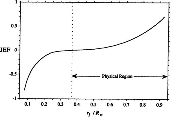
2-3. [JEF] variation with flow ratio (rl/R) ... 26

2-4. Power dissipated by a hydraulic jump ... 29

2-5. Shear induced frictional losses compared to jump dissipation ... 30

3-1. Steady state velocity vectors -- rotor and stator ... 33

4-1. Centerline of blades defined by Base and Inner curves ... 38

4-2. Pictorial representation of Base curve development scheme ... 39

4-3. Trace curve specification in Zo-S plane ... 40

4-4. Cylindrical coordinate system... 41

4-5. Discrete Base curve and direction vectors... 43

5-1. Profile view of the Test Set and nozzle ... 47

5-2. Test Bed showing nozzle angular displacement and linear offset scales ... 48

5-3. Test Section profile and free surface angle convention ... 50

6-1. P* and k variation with Re, for fixed %-Fill ... 55

6-2. P* and k variation with %-Fll, for fixed ... 56

6-3. P* and k variation with N, with all other parameters held constant ... 57

6-4. P* and k variation with B.P., with all other parameters held constant ... 58

6-5. P* and k variation with E, with all other parameters held constant ... 59

7-1. Radial pressure gradient across recirculating liquid flow ... 63

7-2. Rotor and stator blade cutback scheme... ... 64

7-3. Solid body blade shape and tapering scheme ... 65

7-4. Some possible fill conduit locations ... 66

7-5. Performance map of dynamometer ... 68

8-1. Low-speed prototype predicted performance map ... 73

8-2. CAD image of the rotor and stator . ... 74

8-3. Sectional sketch of the low-speed prototype ... 75

8-4. Low-speed prototype experimental set-up. ... 76

8-6. Friction factor variation with Re ... 80

8-7. Low-speed prototype empirical performance map ... 80

8-8. Comparison between measured power absorption & modifiedpredictions ... 81

8-9. Non-dimensional performance map ... 82

8-10. Comparison of predicted and measured static pressure rise with co ... 83

8-11 . Radial velocity profile at different speeds, for 100 %-Fill... 84

8-12. Power supply step on test ... 85

8-13. Power supply step off test, with unloaded and fully loaded dynamometer. ... 86

8-14. Rapid aperiodic rotor speed oscillation test ... ... 87

9-1. CAD representation of full-scale prototype... ... 90

9-2. Predicted full-scale performance map ... 92

9-3. Modified estimated full-scale performance map ... 93

Nomenclature

Transformation variable

Steam vent area

Total acceleration vector Flow cross sectional area

Wetted surface area Unit acceleration vector Damping coefficient

Rotor and stator blade turning angle Blade packing

Curvatur vector Drag coefficient Unit curvature vector

Directional vector

Outside diameter of dynamometer Hydraulic diameter

Unit direction vector Surface roughness

Energy rate out of hydraulic jump Jump energy rate out per unit width Free surface angle, Ch. 5

Friction factor Steam property

Circulation

Fluid drag force

Blade heighth

Latent heat of vaporization Wetted blade heighth Stagnation enthalpy rate

Tangential unit vector Inner curve vector Rotational inertia Recirculation factor Transformation variable

Liquid level in dynamometer

Mass flow rate Number of blades

Liquid kinematic viscosity Dynamometer power absorption Dimensionless power Pressure Pb V

r

r

rl Ro

r

R R' Re rO Rs s

p

t T TZ 0 U

U

V Ve Vrn Vt V Vm Vx W X

X'

Y

y

Z Z' ¢ Blade pitch

Blade rake angle

Radius to point in fluid sheet, Ch. Radius to free surface, Ch 2 Radius to point in liquid sheet

Cylindrical radius, Ch. 2

Torus minor radius Torus major radius Transformation variable Reynolds number

Radius from center of rotation Steam property

Spacing between blades Liquid density

Time, Ch. 10

Maximum blade thickness Rotor torque

Torque applied about z-axis Nozzle relative angle, Ch. 5 Wall shear stress

Rotor blade tip speed

Blade tangential velocity vector Recirculation velocity

Angular velocity

Relative normal velocity Tangential velocity

Base curve position vector

Absolute velocity vector

Liquid volume

Velocity magnitude

Unit velocity vector Relative velocity vector Rotor angular speed

Space curve coordinate

Base curve coordinate Space curve coordinate Base curve coordinate

Space curve coordinate

Base curve coordinate Polar angle aX A A A A. B B B.P.

c

Cd Cae

d

D

dh D 6

r

Fd h hli hw t.

I

J

k L %-Fill

N

V

P

p

CHAPTER 1

Conceptualization of Recirculating Flow

Steam Generating Dynamometer

1.1 Background

The main function of a shaft-power absorbing dynamometer is to produce a load torque to simulate a duty cycle for developmental and/or diagnostic testing of shaft-power producing engines or machines. There are many different kinds of dynamometers available today that operate according to various physical principles and collectively offer a wide range of power absorption conditions. Some well known examples are, electric eddy-current brakes, viscous shear plate absorbers, perforated disc evaporators, and Froude type water brakes, to name a few. However, these devices generally suffer from at least one of the following problems; lack of portability due to low power density (i.e., large size and weight), complex or costly external apparatus required for operation (e.g., heat

exchangers, pumps, or condensers), cavitation erosion which shortens mechanical life of integral parts, or the performance envelope is simply too limited.

In an attempt to overcome these problems Textron-Lycoming (a gas turbine engine manufacturer that is now part of Allied-Signal) developed a preliminary steam generating dynamometer prototype based on the available body of dynamometer knowledge. While the device successfully generated steam, the quality of the effluent was lower than anticipated (iLe., liquid water sprayed out with the steam because of the large degree of blade incidence), resulting in a undesirable large feed-water requirement. Furthermore, there was a significant amount of erosion concentrated in one area of the vanes. Therefore, a need was realized to develop a logical and rigorous method for the design of a portable high-power-density dynamometer that would more successfully overcome the problems described above. This need is the fundamental motivation for the work presented here (which was funded largely by Textron-Lycoming).

The first task was a review of fluid dynamometers in the technical literature, to determine if there were any tools or techniques that could be used here. The conclusions of this

literature survey are summarized as follows. Traditional or commercially available fluid

mechanisms; viscous shear, cavitation, incidence, or momentum transfer by hurling fluid between a rotor and stator (possibly several stages).

For example, in a viscous shear plate absorber a large plate (or disc) is mounted to a rotor in close proximity to a stator and immersed in a bath of liquid. As the rotor spins the disc (or discs) develop a shear stress that leads to viscous dissipation in the fluid. Cool fluid must continually replace hot fluid which can be either dumped to a sink or fed through external equipment, cooled, and recycled. However, in order to get high power absorption levels the shear surface area must be extensive, resulting in a large and massive

dynamometer. Other problems with this type of machine are that the performance envelope is very narrow which limits its utility, and the external equipment required for continuous operation makes the device bulky and impractical to transport.

The perforated disc evaporator functions in the same basic way except that the plates (or discs) have holes bored in them to induce cavitation. The cavitation augments power dissipation and thus reduces the overall size of the machine. Vapor that is generated as power is absorbed can be either vented straight into the atmosphere or condensed and recycled through external equipment. The main problems with this device are vibration and cavitation erosion which results in excessive mechanical wear and thus frequent part

replacement. The current status of these cavitating devices is concisely summarized by

Courtney [11].

Less self destructive machines are the Froude type water brakes. These devices consist of a fluid filled toroidal working compartment, much like a fluid coupling or torque converter, that is split into two halves (generally equal in volume and shape) forming a rotor and stator. The rotor has radial vanes (or some deviation thereof) that spins or hurls the liquid into the stator stage, which may also have vanes. The device absorbs power primarily through incidence resulting from the liquid impingement on the vanes, and to some extent viscous friction. Theories have been developed and experiments executed by Raine [2] and

Shute [3] that are a good source of information for modeling or sizing standard

Froude-type water brakes. These devices have existed for a long time and, over the ages, many attempts have been made to improve performance by varying the number, position, shape, and angle, of the vanes such as the work presented by Patki and Gill [4] and others. Most

of the analyses or experimental data presented in the literature is for fully filled machines.

Some recent work by Raine and Hodgson [5] formalizes the current status of these Froude type machines, and presents an analytical method for predicting performance of both fully

and partially filled liquid water brakes. Unforunately, Froude type water brakes suffer from low power density, erosion, and a performance envelope that is too limited to meet the requirements of modern gas turbine engines (although partial fill improves this). The material reviewed in the literature was not directly applicable to the development of the type of dynamometer required for this application. This substantiated the need for the work reported here.

Simply stated, the objective of this work is the development of a new type of hydraulic dynamometer that is suitable for the diverse range of power levels and high rotor speeds associated with modern gas turbine engines, as well as a method for the design of these new turbomachines. The desired characteristics of the dynamometer are long-life, transportability, high-power-density, and a wide operational envelope.

1.2 New Dynamometer Concept

To accomplish this objective a new type of dynamometer has been developed that functions by developing an organized high-speed free-surface liquid flow that helically. recirculates on the inside surface of a torus. An impeller (or rotor) is used to accelerate the liquid. to a high speed at which point rotor power input is absorbed by primarily viscous dissipation in the recirculating stream. The thesis develops an appropriate geometric configuration and blading scheme that produces this flow.

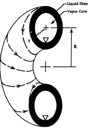
In order to have viscous dissipation as the primary power absorption mechanism, a high speed recirculating flow must be generated. A torus, which is particularly well suited for a recirculating flow, was selected as the working compartment geometry, although there are several other possible geometric configurations that could have been used. This flow can be visualized as a sheet of liquid that helically swirls around, or recirculates, on the inside surface of the torus. The liquid is accelerated by a bladed rotor (which is part of the torus) and is held against the toroidal surface by a strong centrifugal field. A large radial pressure

gradient that results from the streamline curvature of the liquid flow stratifies the fluid by

density resulting in the evolution of a vapor core surrounded by a liquid sheet, as shown in Figure 1-1. As vapor is generated it is vented through radial holes in the blades (described below) that cut through the liquid layer into the vapor core. Furthermore, due to the

Sheet

Core

Figure 1-1. Vapor-liquid stratification in torus

presence of this large radial pressure gradient, boiling is confined to a relatively thin layer

of the liquid sheet near the free surface. The power absorption in this device is clearly

related to the amount of liquid water in the toroidal working compartment (or thickness of

the liquid sheet) and the fluid recirculation velocity.

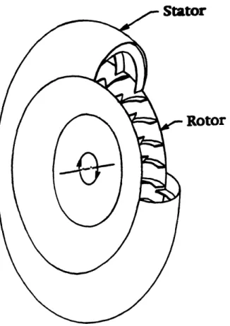
A unique blading scheme has been developed that produces this phase separated helical

flow. The torus is divided in two parts (or stages), a bladed rotor stage and a bladed stator stage. The rotor is the inner part of the torus, or region inside the major radius, and the stator is the remainder of the torus, as depicted in Figure 1-2. The liquid flowing between

the rotor blades is accelerated and exits into the inlet of the stator stage. The liquid flows

the rotor stage where the process continues. The liquid in this flow circuit accelerates until the power dissipated by viscous shear equals the power input by the rotor. The rotor torque input, recirculating mass flow rate, and power dissipation, are all coupled to the

4.d FUAp

Rotor

Figure 1-2. Toroidal geometry with rotor and stator blading

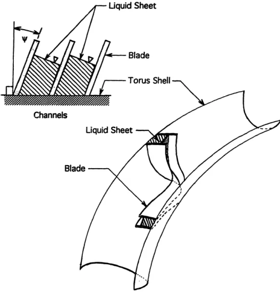
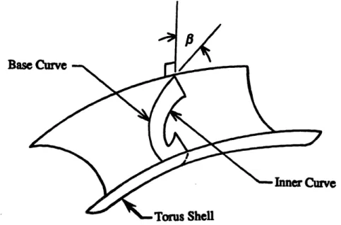
geometric profile (or turning angle) of the rotor and stator blades. However, to make the liquid flow smoothly through this turning angle, the blades must be oriented (defined by rake angle) properly at each point throughout the flow circuit. In other words, the blades must act effectively as the walls of channels in which the liquid flows, as depicted in Figure

1-3. Developing blades in this way reduces the propensity for incidence and cavitation, which is undesirable because it results in localized mechanical wear or concentrated erosion.

The appropriate blade turning and rake angles (which define the shape of the blade) are determined from mass, momentum, and energy conservation, as well as the concept of geometric principle curvature. The turning angle (1P) is defined as the angular change in

S : .! . L -a Sneet Blade -1" . _ CL 11 Channels Liquid Sheet -- \ Blad

Figure 1-3. Channels formed by blades

direction that the liquid flow undergoes between the inlet and outlet of either stage. The

rake angle () is defined as the angle between the blade and a line perpendicular to the torus

shell, as shown in Figure 1-3. A blading algorithm and quantitative techniques have been developed in the thesis for the rigorous determination of blade shapes (defined by 3 and V)

that produce this high-speed helically recirculating liquid flow. The advantages of a

1.3 Resulting Advantages

There are several advantages that result from a dynamometer that operates based on this unique liquid flow. Clearly, by utilizing the liquids latent heat of vaporization the dynamometer power density is quite high. Furthermore, configuring the rotor and stator

stages and blading in this way results in several practical benefits.

The power density of this dynamometer is much higher than conventional (non cavitating) liquid dynamometers because a portion of the recirculating liquid stream undergoes a phase transition. Furthermore, nearly pure steam generated as power is absorbed collects in the inner part (or core) of the torus that can be accessed with the stator blades and vented straight to atmosphere. This not only reduces the feed-water requirements (because the steam quality is high), but also eliminates the need for bulky external support apparatus. The combination of these feature results in a high-power-density dynamometer that can be easily transported. This is particularly beneficial for diagnostic testing of engines, which is typically done by removing and shipping the troubled engine to a test facility which is extremely costly. A portable dynamometer will greatly reduce the cost associated with this type of engine testing.

The dynamometer power absorption is a function of both rotor speed (w) and liquid level (or volume of liquid) in the working compartment. In other words, at a fixed w the absorption level can be varied by changing the amount of liquid in the working

compartment. Therefore, the dynamometer has a wide range of operation that is suitable for modem gas fueled turboshaft engines.

Another benefit, that results from this rotor-stator configuration, is that the net axial thrust

produced is approximately zero. This clearly reduces the cost associated with

dynamometer fabrication. In a typical Froude type dynamometer axial thrust is typically

handled by designing the machine such that it has two equal (but opposite facing) working

compartments which cancel out each others thrust. This obviously increases the size and

complexity of the device, which is undesirable.

Finally, the dynamometer developed here absorbs power through primarily shear stress induced dissipation, which acts on the entire wetted surface of the machine. Since this organized dissipation mechanism is distributed over a relatively large area, the propensity

for concentrated erosion is minimized and the machine life is considerable increased, which is beneficial for obvious reasons.

1.4 Outline of Thesis

The thesis presents a logical and rigorous method (based on a flow model, blading

algorithm, and numerical programs) that can be used to design dynamometers that develop a recirculating liquid flow, and predict power absorption (P) as a function of rotor speed (w) and liquid level (%-Fill). A blade cascade experiment was conducted and a low-speed prototype was designed, constructed, and tested to validate theoretical predictions and explore the question of dynamic stability. The numerical programs can be used for design, analysis and performance prediction which, in conjunction with the experimental results, serves as a basis for a general algorithm that can be used to design this new type of

turbomachine. Furthermore, some scaling laws are identified which are useful for making rough performance extrapolations. Finally, control issues are explored for a typical engine-dynamometer system and some possible control scenarios are presented that aid in the

application of this new dynamometer.

In Chapter 2, different dissipation mechanisms are examined that can absorb a significant amount of power while maintaining an organized recirculating flow, and quantitative techniques for estimating power absorption are presented. This leads to the development of a flow model in Chapter 3 which equates rotor power input with shear stress induced dissipation, and determines the appropriate blade profiles (fluid turning angles,

3)

that result in this power balance. In Chapter 4 a blading algorithm and numerical programs are presented that were developed here and used to generate rotor and stator blades that have the correct shape (defined by f and

V)

for this device. The programs are included in Appendix B. Then a blade cascade flow visualization experiment was conducted to verify the blading algorithm and examine the impact of varying parameters way off design. The conclusions and results of this experiment are presented in Chapter 5. The experimental procedures and raw data are included in Appendix A.

In Chapter 6 a numerical code is presented that was developed based on the flow model and blading algorithm. Also, some key dimensionless parameters are identified that

characterize this new dynamometer. Among other things, the code can be used to make dimensionless performance estimations, study the effects of parameter variations, as well

as predict P for any particular o and %-Fill. Some examples are presented for the purpose of illustration. The code and a sample run are presented in Appendix C.

The dynamometer code and blading programs form the basis of a rigorous general algorithm, presented in Chapter 7, that can be used to design this new type of dynamometer. A method for liquid filling and steam venting is presented that takes

advantage of the natural phase separation (resulting fronl the large centrifugal field) in the

working compartment. Furthermore, some scaling la tvs were identified that relates P to CA and size (D), which are useful for making rough performance extrapolations. In Chapter 8 the general algorithm is applied to the design of a low-speed prototype, which was

subsequently constructed and tested to verify the basic liquid flow characteristics and explore the question of dynamic stability. The experimental results are presented and

compared to theoretical predictions. This information, in conjunction with the general

algorithm, was used to design a high speed full-scale steam generating prototype which is presented in Chapter 9.

Finally, fundamental dynamics and control issues were explored for a typical engine-dynamometer system, and some possible control scenarios are presented in Chapter 10 to aid in the application of this new dynamometer. Chapter 11 consists of a summary of the main contributions of this thesis, as well as some proposals for future work.

CHAPTER 2

Investigation of Power Absorbing Mechanisms

2.1 Overview

The main task here is to dissipate power in the working fluid of the dynamometer. Enough power must be dissipated so that the dynamometer has a high power density. There are several possible fluid dissipation mechanisms that can be considered, including incidence or shock, frictional drag or shear stress, or dissipation associated with the formation of a hydraulic jump. However, incidence or shock losses are usually caused by fluid

impingement on machine parts resulting in damage, and a relatively short mechanical life, which is inconsistent with the fundamental objective. Conversely, the latter two dissipation mechanisms can be generated in an organized (much less destructive) flow and can absorb significant amounts of power. Therefore, hydraulic jumps and wall shear stress are investigated in the following sections as potential power absorption mechanisms.

2.2 Hydraulic Jump Induced Dissipation

Inside the dynamometer there is a centrifugally accelerated two-phase, helically swirling, free surface flow. Since the flow has a free surface, it is capable of spontaneously hydraulically jumping to a lower energy state, which can be exploited as a power

absorption mechanism. To precisely model a hydraulic jump in this complex toroidal flow would be extremely difficult and unnecessary to capture the essence of the jump. Instead, the jump behavior is explored in a cylindrical system, concentrating on the important

fundamental characteristics without complicating the equations with the toroidal geometry.

This is a reasonable approximation since the flow's helical progression speed is (by design) small compared to its angular (tangential) velocity (Ve) component around the minor

dimension of the tomrs.

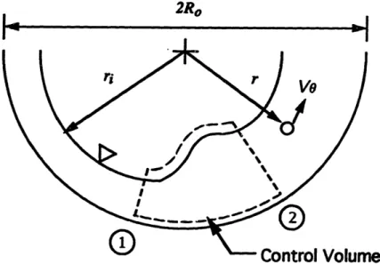
Therefore, the first step to modeling a hydraulic jump in the dynamometer is to unfold the torus into a right circular cylinder and focus on an infinitely thin cylindrical section, see Figure 2-1. Then, the velocity field in the flow circuit must be modeled. Since the

Reynolds number for this flow is very large (by design), the liquid can be approximated as inviscid, except within a very small boundary layer that can be safely neglected here

2Ro

L

I

%.AIILIUI VUiUI II

Figure 2-1. Modeling a hydraulic jump in cylindrical coordinates

because it has little impact on the jump. To conserve angular momentum the angular velocity of a fluid particle times the radius (or distance from the center or rotation to the particle) must be constant. This is the well known Free Vortex solution to Euler's Equation

(in streamline coordinates) for steady incompressible flow,

C

V,=--

(2.1)

r

(2.2)

where the constant is proportional to the circulation (), and the radial and axial components of velocity are negligible compared to the angular component.

The radial pressure gradient (traversing the liquid sheet) can be described in terms of the angular (tangential) velocity, using Euler's Equation in streamline coordinates.

a

=p(V,)2 _pr2

dr

r

4r

2

r

3 (2.3)

___

- --1 I %9%

Since the rate of pressure change in the radial direction is much greater than in any other direction the partial differential equation can be reasonably approximated by an ordinary differential equation. The radial pressure distribution is determined by integrating this equation from the inside free surface of the flow (ri) to any point (r) within the liquid sheet.

|fdp=pI

f

l4

(dr/r3)

(2.4)

r2 ( 1

p,(r) = p(r)-p =p-,(-

-2

(2.5)

The gage pressure distribution (pg(r)) is relative to the core pressure (Po), which is assumed to be atmospheric. The (gage) pressure distribution is used subsequently to evaluate the angular momentum and energy equations across the hydraulic jump. But first continuity must be addressed.

Clearly, the mass flowing upstream (pre-jump) of the hydraulic jump must equal the mass flowing down stream (post-jump), neglecting the mass leaving as vapor which is several orders of magnitude smaller than the liquid terms (again by design). Furthermore, since the normal velocity component is approximately equal to the angular velocity at any point in

the liquid sheet, the mass flow rate in the circuit per unit width of the cylinder can be

evaluated as follows.

ma = *m = m = p

Vedr

= d ln(Ro/r,) (2.6)

The circulation can be solved for using this expression, and noting that the mass flow rate per unit width divided by the density is the volume flow rate per unit width (Q').

r

=

2( Q

(2.7)

Now the angular momentum across the hydraulic jump can be readily evaluated. The

Angular Momentum Theorem states that the rate of change in angular momentum in a given

control volume, plus the net efflux of angular momentum across the control surface, must equal the total torque acting on the control volume. In the steady state case, the net rate of change of angular momentum in the control volume is zero. Therefore, the angular

momentum equation can be written in standard notation for the control volume shown in Figure 2-1 as follows.

p(r x V)V,,dA = T. (2.8)

The cross product of the radius with velocity is simply equal to the angular (tangential) velocity times the radius to that point in the liquid sheet. The relative normal velocity (Vr) is also equal to the angular velocity. The torque applied to the control volume (neglecting skin friction) results from the different pressure forces acting on opposite sides of the jump, due to the difference in pre and post jump liquid sheet thickness. Therefore, the angular momentum equation for the hydraulic jump in this cylindrical system can be expressed as follows.

1P(rV3)dr- 2p(rV 2)dr = rpdr- rpdr (2.9)

Where the numbers 1 and 2 designate pre-jump and post-jump respectively as shown in Figure 2-1. Combining this with Equations (2.1), (2.2), and (2.5), transforms the angular momentum equation into a more useful form.

f!p

,,

2d r

3

_ f

rY

r2dr= f

Jr

P(i2

2 1

i)dr

1

-Jrp1

.

I

-

I

1dr

dr (2.10)

rrr 2 r2 8r

t

r? rsr

Where again ri is the radial distance from the cylinder's center to the free surface and R is one half of its diameter. This integral can now be directly evaluated.

2 lRi) 4r2 _R2)

_(2.11)

4 I

2

,r2J

[

_16r

r (R2_1)_

2 _ri

L'

L

_81r

2 In(R°)]

2 _{r2J 16t}2

r

(

_r-)

,

1)-

_8r2

ln(R-)]

_r

₎

(2.11)

This equation can be simplified by collecting common terms, as in Equation (2.12).

,[12/

n )

+

(rF

-

r1)]

F.I2lnr)

)R+ -1)]

(2.12)

This can be further simplified by using Equation (2.7) to eliminate the circulation terms.

21)+

(

-[14R.)

R,2!

2[

+

J

1

=2 -2(R) (2.13)

Interestingly, from the Angular Momentum Theorem it is clear that a hydraulic jump in a cylindrical system is independent of the mass flow rate, with respect to the post-jump liquid sheet thickness. This means that the post-jump liquid sheet thickness h2(equal to Ro-r2) is

uniquely determined lby the pre-jump thickness hi (equal to Ro-rl). Of course hi (and thus the input radius ratio rIlRo) depends on the mass flow rate or, more specifically, the

recirculating mass flow rate. Furthermore, one side of equation (2.13) contains all of the information needed to completely characterize the hydraulic jump, and is an

non-dimensional number that shall be referred to hereafter as the Jump number or Jump Function [JF]. Figure 2-2 shows how the Jump Function varies with flow ratio rlRo over

a wide range of values. From the figure it is clear that for any flow ratio other than 0367 there are two solutions to the Jump Function. However, only one solution is physical

0.1 0.2 0.3 0.4 0.5 0.6 0.7 0.8 0.9

rlR,

and does not violate the Second Law of thermodynamics. The same holds true for a linear hydraulic jump in a rectangular channel, which can only spontaneously jump from a (high energy) super-critical flow to a (low energy) sub-critical flow. The difference in kinetic energy is equal to the heat added to the water. In a linear hydraulic jump the characterizing parameter is the Froude number, while in a cylindrical system the equivalent parameter is the Jump number (or Function). If the Froude number is greater than one, or in the cylindrical system the Jump number is greater than 0367, then the flow is super-critical and a hydraulic jump is possible. A spontaneous jump in the opposite direction is not physical.

To clarify this a little further look at Figure 2-2 again. Envision a vertical line parallel to the ordinate that passes through the 0367 point on the abscissa (represented by a broken line in the figure). The line cuts the space into two regions. The region on the right side of the line is the physical solution space, which means if the flow has a radius ratio greater than

0367 then a spontaneous jump is possible. If a jump occurs, then the post-jump liquid

sheet thickness can be easily evaluated by determining the radius ratio on the left side of the solution space that corresponds to the same Jump Number in the physical region.

Now that the jump characteristics have been quantified, the power dissipated (as heat) by the jump can be examined. Consider again a control volume that surround a hydraulic jump in a cylindrical system. Using the First Law of thermodynamics, for a steady bulk

flow process, the following observations can be made. The difference in the stagnation

enthalpy rate between the pre and post-jump liquid sheets must be equal to the energy (heat) rate out of the control volume.

to=o

where

H.= mu+R+ V2J

(2.14)

P 2

It is reasonable to assume that the hydraulic jump will occur at near isothermal conditions in the steady case, since the objective is to induce boiling in the vicinity of the jump. Thus,

the specific internal energy will be the same on both sides of the jump and cancel out of the equation. Therefore, the energy balance across the jump can be written in integral form as

k

(pw

dii

-

+

d2i

(2.15)

Consider one of the integrands of this equation, with the previously derived expressions

for p(r) and V(r) substituted in.

p+

2=

r 2 (ii' + 2

L .r

(2.16)

p 2

o7&r\

rr/o

r

Wr

Interestingly, the integrand is only a function of the circulation and radius to the free

surface of the liquid sheet (a constant input parameter), and is independent of the radius to a fluid particle inside the liquid. Substituting Equation 2.16 into 2.15 yields the following energy balance on a per unit width basis.

u=

nit width P = 2r?)27 r 8r2

2

Again, rl and r2 are the radial distances from the center of the cylinder to the free surface before and after the jump respectively, and Ro is half of the cylinder's diameter. Evaluating the integrals in Equation 2.17 yields an expression involving logarithmic functions of the up and down stream radius ratios.

.En

(

)

_)rIn(r)

(-p1r2

_

r

(2.18)

EX r2 82r 2 r2

The energy equation can be further simplified by substituting in Equation 2.7 and collecting similar terms.

E= P(Q) P(Q (2.19)

=

)

L Lr2jj

(2.20)

Notice that the right hand side of the equation can be computed from exclusively angular momentum results. Physically this number is the fraction of the initial (or pre-jump) head

that is irreversibly converted into heat by the hydraulic jump. Hereafter this number is referred to as the Jump Energy Fraction (or Function), abbreviated simply as [JEF].

The results of evaluating the [JEF] over a wide range of values is plotted in Figure 2-3. For any flow ratio the [JEF] is easily determined. But again, only input radius ratios greater than 0.367 (supercritical flow) are valid (i.e., can jump to a lower energy state). The physical space here is the positive region of the solution space, or everything to the right of (rIRO)=0367. This one-dimensional cylindrical hydraulic jump model can now be used to estimate how much dissipation will occur in a dynamometer utilizing a jump to absorb power - neglecting other loss mechanisms.

-r 'r'

0.1 0.2 0.3 0.4 0.5

r 111R.

0.6 0.7 0.8 0.9

Figure 2.3. [JEFJ variation with flow radius ratio (rllR) 0.5 JEF 0- -0.5-I * -k Physical Region -1 I. I ---J I · II . a . . . I

To proceed, consider the rotor blades in the cylindrical system to be approximated by a cascade of linear blades. That is, in the proximity of the rotor blades unwrap the cylindrical flow circuit and treat it as a linear flow system, which is a reasonable estimation technique for a first approximation. This simplifies the equations by permitting the rotor power input

to be estimated with a linear momentum balance across the blades. Then the force (F) exerted by a rotor blade on the flow can be written as follows, where Vtl and Vt2 are the

F = rh(VI - V.I) (2.21)

tangential velocities at the blade inlet and outlet respectively. Equation 2.22 is the mass flow rate per blade pitch (Pb),

th = PhPbV I (2.22)

where h is the liquid sheet height (or thickness) through the rotor stage, Pb is the pitch (blade spacing) and Vnl is the normal component of velocity at the rotor inlet. The

difference in tangential velocity is approximately equal to (by design) the average rotor

blade velocity (U). Combining this with Equation 2.21 yields an expression for the force acting on the rotor blade, in previously determined variables.

F phpbVU

(2.23)

The rotor power input per pitch (P') is equal to the force per pitch multiplied by the average rotor blade velocity.

P = F - phVIU22 (2.24)

Pb Pb

Non-dimensionalizing this yields the dimensionless power (P*) input to the rotor (per pitch), which is clearly a function of liquid sheet heighth (h) and velocity ratio (Vnl/U).

P ReU3P =I ( U) I= Ci ) (2.25)

Since all the rotor input power is assumed to be absorbed in the jump, Equation 2.24 must be equal to jump energy rate (E), which can be extracted from Equation 2.20.

ph2 V3,U2= p(Q'3[1{F] (2.26)

Since the volume flow rate per unit width (Q') is equal to the heighth (h2) times the normal velocity (V=V2=Vnl), this expression can be further simplified.

h2V 1U2= "[~1 (2.27)

Rearranging terms gives the following compact form of the energy balance between rotor input and jump output.

(u)

2(h[JEF] (R - r)[JEF (2.28)

2relJ

2r ln(

n

This relationship combines the results of the angular momentum analysis with the power balance between rotor input and jump dissipation. The (recirculation) velocity ratio can be

computed from this equation, once the jump is characterized, and used in Equation 2.25 to

compute the dinimesonless power input to the rotor, which is equal to the power dissipated by (in) the dynamometer,

This information can now be used to estimate power dissipation for different rotor speeds. But first, some rough machine (toroidal) dimensions must be selected for a hypothetical dynamometer. The toroidal major radius is selected to be 6 inches, and the minor radius 3 inches. Therefore, the cylindrical diameter is 6 inches, and the dynamometer outside diameter is 18 inches. Furthermore, water is selected as the working fluid in this hypothetical case.

Figure 2-4 is a plot of the power absorbed in this hypothetical dynamometer by a hydraulic jump over a wide range of rotor speeds. The power curve is more accurate at low rotor

0 1000 2000 3000 4000

co (rpm)

5000

Figure 2-4. Power dissipated by a hydraulic jump

speeds because at high rotor speeds the jump dissipation rate becomes so high that

appreciable mass leaves the jump in the form of vapor. Thus, at very high rotor speeds the analysis breaks down somewhat, but is still a reasonable and conservative first order tool for estimating power absorption by this particular dissipation mechanism. In the above analysis the losses associated with skin friction were neglected. However, at high speeds these losses are not small, and in fact may be quite large, which is the subject of the next section.

2.3 Shear Stress Induced Dissipation

In the previous section a hydraulic jump was investigated as a potential power dissipation mechanisms for the dynamometer, neglecting any contribution from skin friction. Clearly, as the rotor speed increases the recirculation velocity (which is approximately normal to the

blade rotational velocity) must also increase. At some point the skin friction induced dissipation must become significant, and can in fact be more effective than the jump as a power absorber. This is discussed below, as well as the conditions that are required to produce significant frictional dissipation.

The viscous losses in the recirculating liquid sheet can be estimated by calculating the skin friction drag acting on the wetted surface of the flow circuit. The drag force (Fd) can be written as follows, where p is the liquid density, As is the wetted or shear surface area, Cd is the average drag coefficient, and V is the (recirculating) liquid stream velocity which can be expressed as a factor (k) times the average rotor blade speed (U).

F, = pACdV2 = pA.Cd(kU)2

2

2U

(2.29)

Clearly, the power dissipated by friction is simply the drag force Fd multiplied by the recirculation velocity V.

0 1000 2000 3000 4000

o (rpm)

5000

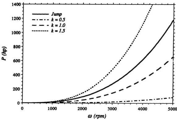
To get some tangible dissipation estimates, consider again the hypothetical dynamometer discussed in the previous section. The wetted surface area can be approximated as the surface area of the torus and the average drag coefficient can be conservatively estimated to be 0.01. With these approximations the shear induced frictional power dissipation can be evaluated. Figure 2-5 shows the power dissipation for several different recirculation factors (k), compared to the power absorbed by a hydraulic jump, over a wide range of rotor speeds. Notice that the shear induced power dissipation surpasses the hydraulic jump dissipation when the recirculation factor reaches a value somewhere between 1.0 and 1.5. In other words, for high recirculation factors the power dissipated by skin friction is more

substantial than the power absorbed in a hydraulic jump.

Theoretically both dissipation mechanisms could be used to absorb substantial amounts of power. However, practical implementation of a hydraulic jump in a toroidal system is

extremely difficult. The first question is how to design the blades so that a sub-critical flo, is accelerated to a super-critical flow, without promoting destructive cavitation. The next

question is how to control the jump to ensure that a jump occurs consistently in the

appropriate location. Weirs can be used but would cause mechanical erosion, especially at

high rotor speeds, which is inconsistent with the fundamental objective here. Furthermore, as aforementioned, at high rotor speeds the jump equations developed in the previous

sections break down because as the power absorption rate increases a significant amount of

mass leaves the jump as vapor. Incorporating these effects in a toroidal geometry would be

a highly formidable task, and would most likely lead to impractical dynamometer designs.

Conversely, a high speed flow can be developed in a practical and controllable way that is

capable of absorbing substantial amounts of power through wall shear stress induced

dissipation, while minimizing blade incidence losses and cavitation erosion. Therefore, the dynamometer blading will be developed in a way that produces a recirculating liquid flow

in which wall shear stress induced dissipation acts as the primary power absorption mechanism.

CHAPTER 3

Development of Dynamometer Flow Model

3.1 Basic Flow Model

Power absorption mechanisms were investigated in the previous chapter, and the shear induced dissipation mechanism was determined to be most consistent with the basic

objective of the work presented in this thesis. In this chapter a flow model is developed for the helically recirculating flow dynamometer based on the shear stress induced dissipation mechanism. The flow field in the toroidal dynamometer is clearly very complex and it would be extremely difficult to precisely model a centrifugally accelerated, helically swirling, two-phase free surface flow. Instead, the intent here is to develop a basic model that embodies the fundamental characteristics of the flow, which can be used to make performance estimates.

There are several important features that must be included in the model. Clearly, the speed of the flow (or Reynolds number) is very important, as well as how the flow is accelerated to a steady operating speed. The volume of liquid recirculating around on the inside surface of the torus is also very important, as well as the determination of the appropriate wetted surface area. Furthermore, estimating friction factors for the flow is crucial for determining both the speed of the flow and predicting power absorption. This requires that

the effects of streamline curvature due to the toroidal geometry be incorporated.

To proceed with the development of a basic model recall from chapter one that the torus is divided into two sections, a rotor and a stator, which form a closed flow circuit. The liquid in the rotor stage is accelerated by the action of the rotor. The liquid flows from the rotor stage into the inlet of the stator stage, proceeds through the stator, and exits into the inlet of the rotor, thus completing a circuit. The liquid accelerates unidirectionally (by design) until a steady state speed is reached at which point the power input from the rotor equals the shear stress induced dissipation in the recirculating liquid. As power is absorbed, a portion of the recirculating liquid undergoes a phase transition which must be bled off and

continually replenished with liquid feed-water to maintain steady operation. As a

consequence of the strong centrifugal field, the liquid and vapor self separate, and a liquid sheet is formed on the surface of the torus. The liquid phase portion of the fluid is much denser than vapor and is by far the most significant part of the flow. Therefore, the model

is built on the concept of a recirculating liquid sheet that dissipates power (by predominantly fluid frictional drag) at a rate equal to the rotor power input.

ator

itor

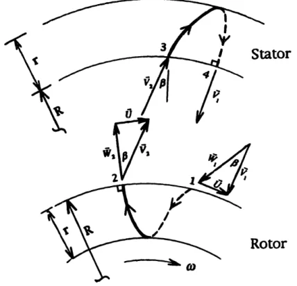
Figure 3-1. Steady state velocity vectors - rotor and stator stages

To accomplish this power balance the rotor and stator blades must have the appropriate turning angles (P), such that the steady state speed (V) of the (recirculating) fluid sheet is related to the rotor blade tip speed (U). This relation is defined here as simply a factor k (refenrred to as a recirculation factor) times U. Figure 3-1 shows the velocity triangles that correspond to the steady state power balance between frictional drag and rotor power input. The liquid in the rotor is accelerated and exits (at point 2) into the inlet of the stator (at point 3). The liquid flows through the stator and exits (at point 4) into the inlet of the rotor (at point 1). The flow continues to accelerate until the power dissipated in the recirculating fluid (by frictional drag) is equal to the rotor power input. Then, by design the steady state change in tangential velocity between rotor inlet and outlet is equal to U. The turning angle

of the blades (P) is related to the recirculation factor (k), and can be calculated from Equation 3.1 below.

tan U = t)a- (3.1)

Since the flow path is closed on itself, and both U and VI are direct functions of ox a fixed turning angle (and hence recirculation factor) can be determined so that the velocity

triangles remain approximately similar over a wide range of rotor speeds. The main objective here is to design the blades so that the fluid exits the stator blades at the correct rotor blade inlet angle, and similarly exits the rotor stage at the correct stator inlet angle. To accomplish this, the correct blade turning angle for both rotor and stator blades should be equal to

fi

as defined above. Clearly, the recirculating mass flow rate in the torus, as well as the momentum and energy exchange between the rotor and liquid, must all be related to (among other things) the recirculation factor (k). These relationships are developed in the following section.

3.2 Power Balance Between Rotor Input and Recirculating Fluid

The liquid in the working compartment is accelerated to a steady state speed at which point the power dissipated by shear stress in the recirculating fluid, neglecting other loss

mechanisms, equals the rotor power input. The liquid flow is modeled here as a pseudo one-dimensional flow, with the effects of the highly twisted streamlines and toroidal geometry included. The blades form channels in which the flow helically recirculates on the inside surface of the torus, see Figure 1-2 and 1-3. The recirculating mass flow rate, torque retarding the rotor, and power absorption rate, are all tied to the recirculation factor

(k) of the liquid in the channels.

The torque acting on the rotor is equal to the net efflux of angular momentum from the rotor stage, and can be determined from elementary turbomachine analysis - expressed as follows.

Due to the closed toroidal flow circuit, the mass flowing through the rotor stage is equal to the recirculation mass flow rate (mi) which can be expressed in terms of the liquid flow cross sectional area (Af), recirculation factor, and rotor blade tip speed (U), as in Equation 3.3 below.

m =pA (kU) (3.3)

Furthermore, Af is equal to the product of the number of blades (N), the flow width or spacing between the blades (s), and the liquid sheet depth or wetted blade heighth (hw). From Figure 3-1 it is clear that the change in tangential velocity is simply equal to the rotor blade speed, and the radius at which the flow enters and exits the rotor is the torus major radius (R). Thus, Equation 3.2 can be re-written as follows, where the term in parenthesis is the recirculating mass flow rate.

T = (pAku)uR _ (pNshkU)UR (3.4)

The torque times the rotor speed (w) is the power input to the fluid through the rotor, which can be expressed in terms of the machine parameters defined above.

P,, = T(o - (pNshkU)UR0

(3.5)

Since ois simply the blade tip speed (U) divided by R, Equation 3.5 can be expressed more succinctly as follows.

P,, = To (pNsh kU)UR(Y) = pNsh.kU3 (3.6)

At steady state, the rotor power input must be equal to the power dissipated by the fluid, which is equal to the drag force (Fd) times the flow speed (V), neglecting other losses. The flow speed is (approximately) the recirculation factor times the blade tip speed. Thus the absorbed power can be written in terms of these parameters, a friction coefficient or factor

(Cd) and the wetted surface area (As), as in Equation 3.7.

The wetted surface area is simply the product of the total fluid path length through the rotor and stator stages, the number of blades, and the wetted perimeter of the channels.

However, the dimensions of the channel change as the fluid travels around the flow circuit due to the toroidal geometry. Therefore, the flow circuit must be broken down into (n) sub-sections, with the wetted surface area (Ai) and friction factor (f) individually evaluated for each sub-section (or locality). Incorporating this into Equation 3.7 yields the following expression for the dissipated power.

fPda-2 =_ Tp(kU)3EdfA, (3.8)

By design, the steady state power dissipated in the dynamometer by frictional drag (Equation 3.8) is equal to the power input by the rotor (Equation 3.6). Canceling terms reduces this equality to a simple form.

Nsh. k2fjA (3.9)

2 i-1

The fluid recirculation factor (k) that equates rotor power input with shear stress induced dissipation can be determined from Equation 3.9. However, the local friction factor (f) is a function of (among other parameters) k, which makes the equation non-linear.

Therefore, Equation 3.9 is best solved iteratively using a computer. An iterative procedure is described in Chapter 6, where a numerical code is presented that was developed based on the model described here. But first a method for predicting the (local) friction factor for the liquid flow is presented.

3.3 Friction Factor Prediction & the Effect of Streamline Curvature

There is no known formula or empirical correlation to accurately calculate the friction factor for this highly twisted, free surface, turbulent recirculating flow. This could only come through the testing of machines that operate on the principles set forth in this thesis. Since

there are no known machines like this, there are no experimentally generated correlations to use. Instead, friction factors are predicted here in a way that is consistent with the flow

model developed above, with the toroidal geometry and effects of streamline curvature incorporated.

Recall that the liquid flow through the rotor and stator stages is effectively a channel flow, with the blades forming the sides of the channels. Clearly, the friction factor for this flow is proportional to the shear stress acting on the wall (i t) and, from dimensional analysis, has a functional form as follows where e is the surface roughness, dh is the hydraulic diameter of the channels, and rc is the radius of curvature of the mean streamline.

f

-

= f(Re

£/

,

d,/2r

(3.10)

To get tangible numbers, a reasonable starting point for approximating the friction factor is the Moody diagram, which presents data forf as a function of Reynolds number and relative roughness (e(dlJ. The Moody diagram is for fluid flow through straight fully wet conduits, but can be used to obtain reasonable approximations for partially filled conduits. To include the secondary flow effects that result from the streamline curvature, the

following correlation from Rohsenow and Choi [6] can be used to modify the friction factor predicted for flow through straight fully wet conduits.

[

[Re(

)

]

2

(3.11)

This relationship is for a fully wet conduit that is helically twisted, but again can be used to

obtain reasonable estimations for friction factors in partially filled conduits, where rc is the approximate helix radius of the mean streamline.

To summarize, the Moody diagram in conjunction with Equation 3.11 provides a means of

estimating the shear stress inducted friction factors in a way that satisfies the functional

relation in Equation 3.10. This technique is used to evaluate Equation 3.9 in the

dynamometer flow code (developed in Chapter 6) but first an algorithm to create blades that

CHAPTER 4

Blade Generation Algorithms & Programs

4.1 Overview

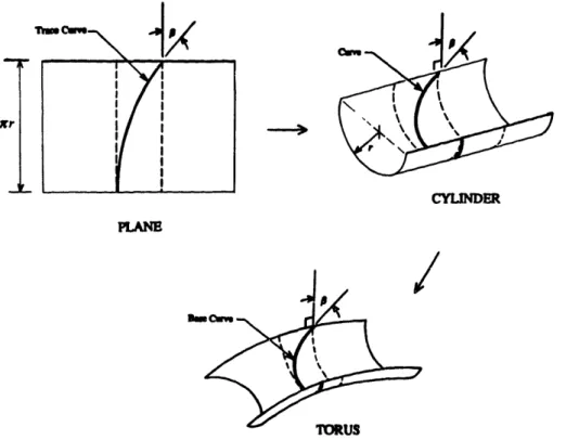
The rotor and stator turning angles (P) are defined by the recirculation factor (k), which is determined from the power balance developed in the previous chapter. The next step is to determine blade profiles that have the correct turning angles. These profiles define the base of the rotor and stator blades, and will thus be referred to as Base curves. This is broken down into two steps. First, a reasonable planar (2-D) curve is selected that can make the liquid flow smoothly through the correct turning angle. This 2-D curve is called a Trace curve, which would exactly define the profile if the flow was planar. But since the flow is clearly three dimensional, the Trace curves must be transformed into the appropriate coordinates. Therefore, the second step is to transform the Trace curve into cylindrical, and ultimately toroidal, coordinates which define the rotor and stator Base curves that lay on the surface of a torus. Then, an Inner curve is developed that together with the Base curve (i.e., connected by a surface) define the centerline (or basic shape) of the blades, as shown in Figure 4-1.

Bas

ve

Figure 4-1. Centerline of blades defined by Base and Inner curves

The blades must be oriented in a way that keeps the liquid in the channels (formed between any two blades). That is, the blades must have the correct rake angle (, defined in Figure

1-3) at each point along the flow path to keep the free surface of the liquid perpendicular to

the blades, just as a roller coaster track must be banked properly to keep the car's wheel force perpendicular to the track. For the stator this is done by determining the direction of principle curvature, at each point along the flow path, and orienting the blades in this direction. The rotor blades are more complicated to account for the acceleration terms

associated with its rotation. Therefore, the rotor blades are oriented parallel to the total

acceleration vector of the fluid particles, instead of in the direction of principle curvature. The result is the same, the free surface of the liquid in the channels is kept approximately perpendicular to blades as the fluid turns through the prescribed angle ((3).

4.2 Base Curve Development

The first step in the blade generation process presented here is the development of a Base curve. To accomplish this, a planar (or Trace) curve is specified that has the appropriate turning angle (), such as a circular :egment cut at the correct point. Then the planar curve is transformed, or mapped, onto the surface of a cylinder. Next, the cylindrical curve is transformed into toroidal coordinates, where the resulting space curve is the Base curve. This scheme is pictorially represented in Figure 4-2, where r is the toroidal minor radius.

xr CYILINDER PANE / , an

Figure 4-2. Pictorial representation of Base curve development scheme

L

I I

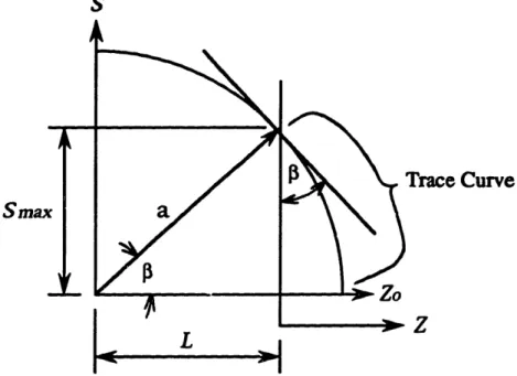
Any planar curve that guides the liquid flow through the correct turning angle (.) can be chosen as the Trace curve and defined in terms of ZO and S coordinates (where ZO and S are dummy variables to be eliminated by transformations). Since this is a planar curve the rotor and stator Trace curves are the same, except that they are complimentary, or 180°

reversed. As alluded to above, the Trace curve selected here is a circular segment of radius

(a) centered at the origin, which can be described by Equation 4.1.

Z

2

_{+ s}

2

_=a

2 _(4.1)

More specifically, the Trace curve is defined as the segment of this circle that produces the correct turning angle (fi). To achieve this, consider another variable Z whose axis is parallel to the Z-axis. The Z-axis is positioned a distance (L) to the right of the origin such

that the angle between the line tangent to the circle (at the intersection point) and the Z-axis

is equal to /, as shown in Figure 4-3.

The parameters needed to describe the Trace curve can be computed from Equations 4.1 through 4.4, where (r) is the radius of a cylinder that corresponds to the minor radius of the torus, which will (together with R the major radius) define the dynamometer's working compartment. Equation 4.2 (on the following page) defines the maximum value of S which clearly must correspond to one half the minor circumference of the to:ms in order to

S

Trace Curve

Z

Figure 4-3. Trace curve specification in ZO-S plane

Sma,

-have a Trace curve that is transfoed onto this cylindrical surface. In Equation 4.3 and 4.4 the variables a and L arc defined by the geometry of the Trance curve, defined above.

Smar = rI

a = SmalSin(P)

(4.2)

(4.3)

L = a(cosfi) (4.4)

Next, the Trace curve is transformed into cylindrical coordinates, such that it lays on the surface of a half cylinder. The transformation equations developed to accomplish this are as follows (Equations 4.5 through 4.8), where X, Y, and Z are the Cartesian coordinates of a point that lays on the cylindrically transformed Trace curve. The X-Y origin is located at the upper left hand point on the half cylinder on which the Trace curve is wapped, and

¢ is the polar angle to a point on the cylindrically transformed Trace curve, as shown in Figure 4.4 (a).

;enur or .ytlmoer

(a)

z

(b)

Figure 44. Cylindrical coordinate system