HAL Id: insu-01514406
https://hal-insu.archives-ouvertes.fr/insu-01514406
Submitted on 26 Apr 2017
HAL is a multi-disciplinary open access
archive for the deposit and dissemination of
sci-entific research documents, whether they are
pub-lished or not. The documents may come from
teaching and research institutions in France or
abroad, or from public or private research centers.
L’archive ouverte pluridisciplinaire HAL, est
destinée au dépôt et à la diffusion de documents
scientifiques de niveau recherche, publiés ou non,
émanant des établissements d’enseignement et de
recherche français ou étrangers, des laboratoires
publics ou privés.
storm: A global multi-instrumental overview
Elvira Astafyeva, Irina Zakharenkova, Matthias Förster
To cite this version:
Elvira Astafyeva, Irina Zakharenkova, Matthias Förster. Ionospheric response to the 2015 St. Patrick’s
Day storm: A global multi-instrumental overview. Journal of Geophysical Research Space Physics,
American Geophysical Union/Wiley, 2015, 120 (10), pp.9023-9037. �10.1002/2015JA021629�.
�insu-01514406�
Ionospheric response to the 2015 St. Patrick’s Day
storm: A global multi-instrumental overview
Elvira Astafyeva1, Irina Zakharenkova1, and Matthias Förster2 1
Institut de Physique du Globe de Paris, Paris Sorbonne Cité, Paris VII - Denis Diderot University, UMR CNRS 7154, Paris, France,2GFZ German Research Centre for Geosciences, Potsdam, Germany
Abstract
We present thefirst multi-instrumental results on the ionospheric response to the geomagnetic storm of 17–18 March 2015 (the St. Patrick’s Day storm) that was up to now the strongest in the 24th solar cycle (minimum SYM-H value of 233 nT). The storm caused complex effects around the globe. The most dramatic positive ionospheric storm occurred at low latitudes in the morning (~100–150% enhancement) and postsunset (~80–100% enhancement) sectors. These significant vertical total electron content increases were observed in different local time sectors and at different universal time, but around the same area of the Eastern Pacific region, which indicates a regional impact of storm drivers. Our analysis revealed that this particular region was most concerned by the increase in the thermospheric O/N2ratio. At midlatitudes, we observeinverse hemispheric asymmetries that occurred, despite the equinoctial period, in different longitudinal regions. In the European-African sector, positive storm signatures were observed in the Northern Hemisphere (NH), whereas in the American sector, a large positive storm occurred in the Southern Hemisphere, while the NH experienced a negative storm. The observed asymmetries can be partly explained by the thermospheric composition changes and partly by the hemispherically different nondipolar portions of the geomagneticfield as well as by the IMF By component variations. At high latitudes, negative ionospheric storm effects were recorded in all longitudinal regions, especially the NH of the Asian sector was concerned. The negative storm phase developed globally on 18 March at the beginning of the recovery phase.
1. Introduction
Ionospheric storm is a common term that describes the entirety of ionospheric variations induced by geo-magnetic disturbances. The ionospheric storms primarily occur as a consequence of a sudden input of solar wind energy into the magnetosphere-ionosphere-thermosphere system. The onset of a geomagnetic storm, when the interplanetary magneticfield (IMF) Bzcomponent turns southward and strengthens, is marked by
(1) largely reinforced auroral particle precipitation and (2) enhanced high-latitude ionospheric currents and convection lasting several hours. As a consequence, the Joule heating and ion-drag forcing, along with the increased high-latitude ionization and penetration of electricfields to low latitudes, significantly affect the global dynamics and structure of the thermosphere and ionosphere. The thermosphere heats and expands, causing storm time neutral winds and generating traveling atmospheric disturbances (TADs), which led to the global changes in the composition and dynamics of both the ionosphere and thermosphere. This, in turn, is the cause of both increases and decreases in electron plasma densities and total electron content (TEC), which are also known as positive and negative storms [Prölss, 1995; Richmond and Lu, 2000; Förster and Jakowski, 2000; Mendillo, 2006; Danilov, 2013]. The negative storms are primarily explained by a decrease of the neutral density ratio O/N2leading to an ion loss rate enhancement [e.g., Prölss, 1995; Fuller-Rowell
et al., 1994]. In contrast, positive storm effects, especially at midlatitudes, remain the most unpredictable feature of the ionospheric storms. Besides an increase in the neutral density ratio O/N2as possible candidate
for the positive storm occurrence, storm time thermospheric winds, prompt penetration, and disturbance dynamo electricfields, as well as plasmaspheric downward fluxes, have been reported to be the main causes of the storm time increases in the ionospheric plasma density [e.g., Fuller-Rowell et al., 1996; Richmond and Lu, 2000; Förster and Jakowski, 2000; Huang et al., 2005; Crowley et al., 2006; Danilov, 2013].
Thus, ionospheric effects of geomagnetic storms have been extensively studied for decades but not yet com-pletely understood. A new multi-instrumental era aids to discover new aspects of the global development of ionospheric and thermospheric storms with better details [e.g., Tsurutani et al., 2004; Yizengaw et al., 2006;
PUBLICATIONS
Journal of Geophysical Research: Space Physics
RESEARCH ARTICLE
10.1002/2015JA021629
Key Points:
• Multi-instrumental analysis of the iono-spheric storm of 17–18 March 2015 • Inverse hemispheric asymmetries in
VTEC in the American and European-African longitudinal sectors • Extreme topside TEC enhancement
over the Eastern Pacific region was observed at different UT and LT
Supporting Information:
• Movie S1
• Text S1, Figure S1, and Movie S1 caption
Correspondence to:
E. Astafyeva, astafyeva@ipgp.fr
Citation:
Astafyeva, E., I. Zakharenkova, and M. Förster (2015), Ionospheric response to the 2015 St. Patrick’s Day storm: A global multi-instrumental overview, J. Geophys. Res. Space Physics, 120, 9023–9037, doi:10.1002/2015JA021629. Received 3 JUL 2015
Accepted 19 SEP 2015
Accepted article online 25 SEP 2015 Published online 26 OCT 2015
©2015. American Geophysical Union. All Rights Reserved.
Foster and Coster, 2007; Goncharenko et al., 2007; Astafyeva, 2009b, 2009a; Lu et al., 2012; Balan et al., 2011; Lei et al., 2014; Astafyeva et al., 2015]. In this paper, we use ground-based GPS receivers, those on board the three Swarm, the Gravity Recovery and Climate Experiment (GRACE), and the TerraSAR satellites, as well as the Swarm in situ measurements to study the ionospheric response to an intense geomagnetic storm that occurred on 17–18 March 2015.
2. Geomagnetic Storm of 17
–18 March 2015: St. Patrick’s Day Storm
The storm commenced on St. Patrick’s Day, 17 March 2015, with the arrival at Earth of a coronal mass ejection at 04:45 UT. The sudden storm commencement (SSC) was marked by a sharp increase in the solar wind speed and pressure as shown in the high-resolution (5 min) OMNI data set provided by the Goddard Space Flight Center (Figure 1a). We note that we had to apply a correction of the time delay that has been estimated as the arrival time at the bow shock nose in the OMNI data set. We shifted Figures 1a–1c by +15 min (toward later arrival) in order to match it with the SSC time observed globally by ground-based magnetometers. According to a statistical study of Case and Wild [2012], a 15 min error is within the error bars of delay time differences that have been obtained independently by cross-correlation estimations with ACE and Cluster observations. We also have to take into account the propagation time of the coronal mass ejection (CME) shock front changes from its arrival time at the bow shock nose to the location of observation by magnet-ometers on ground level, which can be estimated to be of the order of ~5 min [Villante et al., 2004] out of Figure 1. Variations of interplanetary and geophysical parameters during the intense geomagnetic storm of 17–18 March 2015. (a) solar wind speed (Vsw, black curve) and solar wind ram pressure (Psw, blue curve), (b) the IMF Bx(black) and By
(blue) component, (c) the IMF Bzcomponent (black) component, (d) combined polar cap index, and (e) SYM-H (black curve)
and Kp (blue bars) indices. All data are 5 min averaged, except for the PC index (1 min resolution) and the Kp index (3 h). The vertical dashed line shows the time of the SSC of 04:45 UT. For the data of interplanetary parameters, an additional shift of +15 min was applied in order to match the SSC time.
the 15 min time shift. The additional time shift correction might be due to the breakdown of the“planar phase front” assumption at the solar wind CME shock front that is used for the OMNI data delay time estimates (http://omniweb.sci.gsfc.nasa.gov).
The main phase of the storm began at ~ 07:30 UT on 17 March, when the interplanetary magneticfield (IMF) Bz component turned southward for thefirst time and the SYM-H index started to gradually decrease
(Figures 1c and 1e). Shortly after, the IMF Bzturned northward for ~40 min and redropped negative at
~08:30 UT. It was positive again from 10:10 UT to 12:20 UT and prompted a small short time increase in SYM-H. From 12:20 UT, the IMF Bzturned again southward for a longer time and remained that until the next
day. Consequently, the SYM-H continued to decrease and reached its minimum excursion of 233 nT at 22:45 UT on 17 March (Figure 1e). Then a long recovery phase started. The planetary Kp index counted its maximum of 8 from ~12 UT to 24 UT with an intermediate value of 7+ at 18–21 UT on 17 March (Figure 1e). This storm, therefore, was the strongest in the 24th solar cycle at that time.
To understand the energy that enters into the magnetosphere during solar wind-magnetosphere coupling, we analyze variations of the combined polar cap index PC (Figure 1d). One can see thefirst increases of Figure 2. Instruments and data used in this work. Brown pentagons indicate the positions of the ground-based GPS receivers used to plot the meridional chains of VTEC in the American, European, and Asian regions; black triangles indi-cate positions of ground-based ionosondes. Colored curves correspond to the satellite passes at 01–02 UT on 18 March 2015: magenta, TSX; orange, GRACE; green, Swarm C; blue, Swarm B; brown, GUVI; and red—Jason-2. The background color shows values of the VTEC as calculated from the GIM by CODE for 01 UT on 18 March; the corresponding color scale is shown on the right.
Table 1. Summary of the Main Characteristics of the Instruments Used in the Study
Data Source LT Height (km) Orbit/Inclination Measurements/Range Ground-based GPS 0–24 - Global network VTEC (0 ÷ 20,200 km) Ionosondes 0–24 - Global network NmF2(0 ÷ Hmax)
TSX ~18 (ascending) 515 Circular VTEC (515 ÷ 20,200 km) ~6 (descending) Sun-synchronous
97.5°
GRACE ~17.6 (ascending) 410–430 Circular VTEC (43 0÷ 20,200 km) ~5.6 (descending) 89°
Swarm B 21.2 (ascending) 510-520 Circular VTEC (530 ÷ 20,200 km) 9.2 (descending) 87.5° Ne (530 km) Swarm C 19.7 (ascending) 460 Circular VTEC (460 ÷ 20,200 km)
7.7 (descending) 87.5° Ne (460 km) GUVI 9.8–10.2 625 Circular O/N2in column below 625 km
74.1°
Jason-2 ~14.5 (ascending) 1336 Circular VTEC (0 ÷ 1336 km) GPS on Jason-2 ~2.5 (descending) 66° VTEC (1336 ÷ 20,200 km)
the polar cap magnetic activity at ~06 UT and at 09 UT and then four other intense peaks at 14, 18, 21, and 23:30 UT on 17 March. During these periods of time, the PCC index reached 10–15 that indicates an extreme substorm activity during the storm [Troshichev et al., 1988, 2006].
3. Data and Methods Used
To study the ionospheric response to the St. Patrick’s Day storm, we used the following set of instruments (Figure 2 and Table 1):
1. From data of ground-based GPS receivers, it is possible to calculate the slant ionospheric total electron con-tent (TEC), which is equal to the number of electrons between a receiver on the ground and a GPS satellite at ~20,200 km of altitude [e.g., Hofmann-Wellenhof, 2001]. In order to obtain values of the vertical TEC (VTEC) above single GPS receivers, the initial slant TEC data series were further processed into the absolute VTEC by simple geometric factor; the diurnal VTEC variation were further calculated from VTEC series from all visible satellites during 24 h [e.g., Zakharenkova and Astafyeva, 2015; Zakharenkova and Cherniak, 2015]. In addition, in order to have a global overview of the VTEC behavior during the geomagnetic storm of 17–18 March 2015, we used 1 hr resolution global ionospheric maps (GIM) calculated by the Center for Orbit Determination in Europe (CODE), University of Bern from data of ~150 ground-based GPS receivers located worldwide [Schaer et al., 1998] and available from [ftp://cddis.gsfc.nasa.gov/gps/products/ionex/]. The unit of TEC is TEC Units (TECU) with 1 TECU = 1016electrons/m 2.
2. Data of several ground-based ionosondes were used to analyze the behavior of NmF2during the two days of the storm.
3. The VTEC variations calculated from data of dual-frequency GPS receivers on board the three satellites (A, Alpha; B, Bravo; and C, Charlie) of the European Space Agency (ESA)’s recent mission Swarm [Olsen et al., 2013] were used here for thefirst time. Two out of the three Swarm satellites—Swarm A and Swarm C—fly in a tandem separated by 1–1.4° of longitude at an orbital altitude of 460 km, while the third satellite— Swarm B—flies at an altitude of 510–520 km. The orbit inclination is 87.5°. During the 17–18 March storm, the Swarm A and Swarm C satellites crossed the equator at ~19.7 LT (ascending) and ~7.7 LT (descending) and Swarm B satellite at ~21.2 LT (ascending) and 9.2 LT (descending). Because Swarm A and Swarm Cfly the same orbit at almost the same time, their VTEC measurements are almost identical, so here we only show measurements from Swarm C. In addition to the VTEC data, here we used the in situ measurements of the elec-tron density (Ne) from the Langmuir Probe (LP) on board the Swarm satellites. The Ne data are not calibrated yet to the absolute values; however, they can be used to analyze the relative storm time changes.
4. VTEC variations have been obtained from data of a dual-frequency GPS receiver on board the TerraSAR-X satellite (hereafter referred to as TSX). The TSX satellite was launched on 15 June 2007 into a Sun-synchronous dawn-dusk orbit with an inclination of 97.5° (http://www.dlr.de/eo/en/desktopdefault.aspx/ tabid-5725/9296_read-15979/). The satellite crosses the equator at ~18 LT (ascending) and ~06 LT (descend-ing). During the St. Patrick’s Day storm, the TSX satellite flew at an orbital altitude of about 515 km. 5. VTEC calculated from the data of GPS receiver on board the two GRACE (Gravity Recovery and Climate
Experiment) satellites. GRACE-A and GRACE-B satellitesfly at near-circular polar orbits with an inclination of 89°. In March 2015, their orbital altitude is ~410–430 km. During the 17 March storm day, GRACE crossed the equator at ~17.5–17.7 LT (descending passes) and 5.5–5.7 LT (ascending passes).
6. Thermospheric O/N2composition changes as measured by the Global Ultraviolet Imager (GUVI) on board the Thermosphere, Ionosphere, Mesosphere Energetics and Dynamics (TIMED) satellite [Christensen et al., 2003]. GUVI measures a narrow swath below the satellite at 625 km altitude, so that a global picture is accumulated from 14.9 daily orbits. On the 17–18 March storm days, the satellite crossed the equator at ~9.8–10.2 LT during its daytime spectral observations.
7. The dual-frequency satellite radar altimeter Jason-2,flying at a circular orbit at 1336 km altitude, with an inclination of 66° (http://www.aviso.oceanobs.com/en/missions/index.html), provides data of the VTEC between the water/ocean surface and its orbital altitude [Imel, 1994]. In addition to the VTEC data beneath the satellite, we calculate VTEC by using data from the GPS receiver on board the Jason-2 satellite. The latter can be calculated everywhere (including above the continents) along the satellite pass and provides information about changes in the upper topside ionosphere-plasmasphere (above 1336 km). During the March 2015 storm, the satellite Jason-2 crossed the equator at ~14.5 LT (ascending) and ~2.5 LT (descending).
4. Observations
4.1. Global Overview of the Storm Time VTEC Behavior
In order to get an idea about the global dynamics of the ionospheric plasma during the 17–18 March 2015 geomagnetic storm, we first take a look on 1 h resolution global maps of VTEC obtained from GIM by CODE (Movie S1 available as supporting information, upper panel) and on differential VTEC maps calculated as difference between the current VTEC value and the 7 day median VTEC (lower panel in Movie S1). Figure 3. Variations of VTEC measured by the ground-based GPS receivers in (a) American, (b) European-African, and (c) Asian sectors during the 17–18 March 2015 storm (black curves). Names and coordinates of the receivers are shown in each panel. As a quiet time reference, we plot a median for 7 days before the storm (blue curves). Positive and negative deviations from the 7 day median value arefilled by light red and light blue, respectively. The SSC of 04:45 UT time is shown by the vertical dashed lines; the thin gray vertical lines correspond to 00 UT of 18 March 2015.
Following the beginning of the main phase at ~07:30 UT, thefirst storm time VTEC enhancement started to appear in the Northern Hemisphere (NH) from 09 UT, as can be clearly seen from the differential maps (lower panel). During the next 3 h, the dayside VTEC further increased at midlatitudes in both hemispheres. At 13 UT, the storm time VTEC increase became less significant, and at 14 UT we observed a decrease in the differential VTEC localized around low latitudes and in the premidnight (~22–23 LT) sector. Starting from 15–16 UT, and following the second persistent negative IMF Bzevent during the St. Patrick’s Day storm (Figure 1), a new
wave of storm time VTEC changes arrived and lasted until the next day. At 16–17 UT, positive VTEC deviations of up to 70 TECU were observed throughout all latitudes on the dayside. At 18 UT, depletions can be seen over north of North America that extended further southward and intensified from 19 UT onward. From 21 UT on March 17 to 05 UT on March 18, we see a clear hemispheric asymmetry in the dayside storm time VTEC deviations: a strong negative storm in the NH and a strong positive storm in the Southern Hemisphere (SH) over South America. From 06 UT of 18 March, the positive VTEC storm was mostly localized around low latitudes. It lasted until ~12–13 UT. A strong negative storm started to occur at low and midlatitudes of the NH from 01–02 UT on March 18, and surprisingly, it was localized in the prenoon-afternoon sector (~11–15 LT). This negative VTEC deviation further extended toward midlatitudes, in particular, to the SH and occupied a larger longitudinal sector on the dayside. From 15 UT, negative storm effects prevailed, being much stronger at the SH midlatitudes (11–22 UT) as compared to the NH, and by ~23–24 UT on 18 March the storm time effects were less significant. We note that during this storm the differential VTEC reached quite high values: ±68–72 TECU. The absolute VTEC reached a maximum of 120 TECU at low latitudes during the main phase of the storm.
The GIM can be very useful to understand thefirst preliminary overview of the storm time ionosphere redis-tribution. However, it is known that in the GIM the error in the VTEC estimation can be quite significant under certain circumstances, especially over the oceans, where only a few ground-based GPS receivers are located [e.g., Hernandez-Pajares et al., 2009]. Besides, the 1 h resolution might be not good enough to analyze the storm time effects in detail. Therefore, in order to have more precise information about the storm time VTEC changes in different longitudinal regions, we analyze data from other available ground-based and space-borne instruments. Let usfirst examine the variations of VTEC from data for three meridional chains of ground-based GPS receivers (Figures 2 and 3a–3c). In the Asian sector, the VTEC increases at low latitudes shortly after the beginning of the storm at 04:45 UT on 17 March, i.e., at local noon time. At midlatitudes, the small and short-term VTEC increase was followed by a decrease from ~14 UT. At high latitudes, no changes occurred with the storm onset, and from ~20 UT a negative storm commenced (Figure 3c). In the European-African sector, an asymmetrical response is observed. At low and midlatitudes of the NH, a positive storm occurred from 08 UT over all the daytime and evening hours until midnight. At the same time, at equa-torial latitudes and in the SH, no storm time changes, or very small and short-term TEC increases were recorded (Figure 3b). On the contrary, in the American sector, at high and midlatitudes of the NH, a very small short-term increase occurred at ~17–19 UT (near local noon); this small enhancement was followed by a strong negative storm that further lasted all day of 18 March. At low latitudes, the storm time TEC started to increase close to sunrise in this sector at ~14 UT, and with ~30–80% it exceeded the quiet time level. This increase further lasted until ~08 UT of the next day. The largest TEC value of 100 TECU was recorded by the MGRP receiver at ~17 UT. At high latitudes and midlatitudes of the SH, a smaller VTEC increase was observed at 17–23 UT. We point out that at midlatitudes we observe inverse north-south asymmetries in the TEC response in different longitudinal sectors: in the European-African sector, a positive storm was observed in the NH, and almost no storm time changes in the SH, whereas in the American sector, a negative storm occurred in the NH and a positive in the SH. At the same time, at all regions, the high latitudes seemed to experience a negative storm. This negative storm further developed on the second storm day (18 March), when it descended toward middle and even low latitudes (Figures 3a–3c). The negative storm effect appears to be the strongest in the Asian sector (Figure 3c).
Jason-2 provides VTEC measurements in the range 0–1336 km over the oceans, which is supplementary to the ground-based stations. Figure S1a shows that in the ~14.5 LT sector the storm time VTEC increase reached ~25–30% at 20.5–23 UT (tracks 1 and 2); at 02–04 UT on 18 March the VTEC beneath 1336 km decreased by ~10–40% (tracks 3 and 4). Also, we notice the inverse hemispheric asymmetries in the European-African and American sectors during the satellites’ passes in these regions, similarly to the ground-based observations.
The VTEC measurements from the ground-based GPS receivers and those beneath Jason-2 are in good agree-ment with the results from ground-based ionosondes (Figure 4), which means that the observed effects equally concern the ionospheric F layer dynamics and the topside ionosphere, at least locally above the GPS receivers and ionosondes. At the same time, one can also notice gaps in the data of the ionosondes, which occurred due to several reasons. For the South American stations, the determination of the critical fre-quency of the F2layer was difficult due to the presence of an intense spread F, which is a commonly known
feature at low latitudes, especially during geomagnetic disturbances and in the evening time [e.g., Abdu, 2012]. For the midlatitude stations of the NH the data gaps are due to the total/partial absence of the re flect-ing echoes in the ionograms. Such kind of fade-out effect can be related to a significant decrease of the F2
region electron density and/or to an increase in the ionospheric plasma turbulence and D layer absorption, which is often observed during the negative phases of geomagnetic storms [e.g., Lynn et al., 2004; Sojka et al., 2004]. For instance, at the Millstone Hill station such conditions were set for a very long time: from 23 UT on 17 March till 11 UT on 18 March (Figure 4a). This is in line with our observations of very long lasting negative effects.
TEC is an integral parameter equal to the number of electrons along a line of sight from 0 km (for ground-based GPS receivers) up to ~20,200 km (GPS satellites orbit); it is impossible to know the exact altitude of the observed ionospheric disturbances. However, it is generally accepted that the maximum contribution to the TEC is governed by the ionospheric F2layer, with approximately 2/3 of the TEC coming from regions
above the ionization maximum, which is known as the topside ionosphere [e.g., Mendillo, 2006]. It has recently been demonstrated that in some cases the F layer and the topside ionosphere may not react in the same manner during geomagnetic storms [Yizengaw et al., 2006; Astafyeva et al., 2015]. These examples show the importance of a more detailed analysis of the ionospheric response at different altitudes. For this purpose, we analyze data of VTEC from satellite observations allowing sounding of the topside ionosphere. Those will, in addition,fill out data gaps over the oceans, where no ground-based instruments can be installed. Below we analyze separately the storm time variations in the topside ionosphere in different longitudinal sectors.
4.2. Response of the Topside Ionosphere in the Evening and Postsunset Sectors
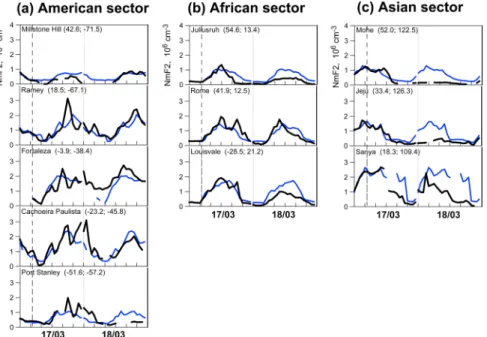
Figure 5 shows variations of vertical TEC measured during the 2 days of the storm by the GPS receivers on board the TSX and GRACE satellites, which passed in close-by local time sectors (equator crossing time Figure 4. Variations of NmF2measured by the ground-based ionosondes in the (a) American, (b) European-African, and
(c) Asian sectors during the 17–18 March 2015 storm (black curves). The quiet time values are shown in blue curves. Names and coordinates of the receivers are shown in each panel. The data gaps at low-latitude ionosondes are due to the spread-F effect; those in the data of midlatitude NH ionosondes are due to the ionospheric plasma turbulence and D layer absorption.
~17.6 LT and 18.00 LT, respectively, see Figure 2) but at different altitudes (~520 km and ~410 km, respec-tively). One can notice that the VTEC distribution is slightly different in the data of these two satellites, which is, most likely, due to the ~110 km of difference in altitude. From ~08–09 UT, a small VTEC enhancement up to ~35–40 TECU in the low-latitude region was observed in both data; however, the effect appeared to be stron-ger and more latitudinally extended in GRACE data (Figure 5b). At ~13–15 UT the VTEC above both satellites decreased to the undisturbed level of ~20 TECU (above TSX) and 30 TECU (above GRACE). Starting from ~16 UT, and following the second IMF Bznegative turning, the low-latitude topside VTEC increased again. From the TSX measurements, the largest topside VTEC increase up to 55–60 TECU was observed from ~22 on March 17 to ~2 UT of the next day (Figure 5a). Compared to the quiet time VTEC values (shown only for the selected orbits 1–4 in Figures 5a (right) and 5b (right) as thin lines), the storm time contribution above ~520 km is estimated as a 100–150% increase within the area of the equatorial ionization anomaly (EIA). The EIA showed a double-peak structure (Figure 5a (right)), most likely, indicating a short-term action of the equatorial electricfields. One can also notice that at midlatitudes the storm time VTEC increase reached ~80–100% in both hemispheres. In the GRACE measurements, the largest enhancement was also observed from ~20:45 UT on 17 March to 01:30 UT of the next day (Figure 5b). During this time, the VTEC above GRACEfirst largely increased in the SH (track 1 in Figure 5b). From 22 to 24 UT, a storm time enhancement of ~80% was observed at low latitudes and midlatitudes (Figure 5b, panels on the right). From 01:30 UT onward, the midlatitude and low-latitude VTEC started to decrease at both height ranges.
Overall, in this local sector, we observe higher storm time increase at midlatitudes in the SH, which is in line with our ground-based observations.
To investigate the storm time behavior of the topside ionosphere in the dusk and postsunset regions, we ana-lyze VTEC data of the Swarm C and Swarm B satellites, which covered the ~19.7 LT and ~21.2 LT regions, respectively (Figure 6). Similarly to the GRACE and TSX observations, thefirst small storm time VTEC enhance-ment was observed shortly after the storm onset at both altitudes and in both longitudinal regions. As in the evening sector, the strongest storm time effect in the VTEC was observed when the satellites passed over the Figure 5. Topside VTEC variations measured by GPS receivers on board the (a) TSX and (b) GRACE satellites in the evening sector on 17–18 March 2015. The black thin curve shows the magnetic dip equator. The color scale for the VTEC is shown next to each panel. The UT and LT of the equator crossings are shown as light blue and black numbers above each satellite pass. The SSC time is indicated by the red arrows with the symbol“SSC” next to them. Small panels in Figures 5a (right) and 5b (right) show latitudinal profiles of the maximum storm time VTEC changes marked by numbers 1, 2, 3, and 4 in Figures 5a (left) and 5b (left) and below the corresponding passes. For comparison, quiet time levels are also shown on the small panels on the right in dark magenta (TSX) or in dark orange (GRACE).
Figure 6. The same as Figure 5 but for the satellites (a) Swarm C and (b) Swarm B in the dusk and postsunset sectors, respectively. The quiet time levels are shown in Figures 6a (right) and 6b (right) in dark green (Swarm C) or in dark blue (Swarm B).
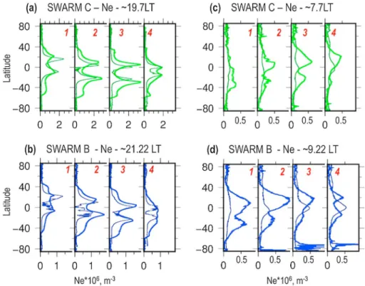
Figure 7. Latitudinal profiles of the in situ electron density measured by the (a and c) Swarm C—green curves and (b and d) Swarm B satellites—blue curves; the quiet time levels are shown by thin dark green and dark blue curves. The corre-sponding satellites tracks are indicated by the numbers 1, 2, 3, and 4 in Figures 6a and 8a and 6b and 8b.
American and Eastern Pacific regions, from ~22 UT of 17 March to 01 UT of 18 March in data of Swarm C satellite and from ~00 UT to ~03 UT on 18 March in the data of Swarm B satellite (Figure 6).
One can also notice that besides the low latitudes, the storm time effects in this region significantly touched the midlatitudes of the SH in particular, so that the effects are not hemispherically symmetrical. For instance, above 460 km (19.7 LT, Swarm C), the ~100% TEC enhancement at midlatitudes appeared from 23 UT (Figure 6a (right)), while above 510 km (21.2 LT, Swarm B), the storm time TEC ~60% exceeded the quiet time levels (Figure 6b (right)). In the 21.2 LT local sector, the signatures of the topside TEC enhancement lasted somewhat longer than in the evening and dusk sectors.
Starting from ~03 UT on 18 March, and when all satellites sounded the Asian-Australian region, the VTEC decreased dramatically at all latitudes. All these satellite measurements in the evening sector confirm our observations from ground-based instruments, including the hemispheric asymmetries: in the European region, a positive storm prevails at midlatitudes in the NH, and a small negative storm can be seen at high latitudes. The situation changes when the satellites approach the Atlantic and American regions, where a stronger positive effect in the SH is observed.
In addition to the VTEC data from the Swarm satellites, here we use in situ electron density (Ne) data mea-sured by the LP of the Swarm satellites (Figure 7). One can see that in both the evening (Figure 7a) and the postsunset (Figure 7b) sectors, the storm time Ne behavior is quite similar to that of the VTEC: we observe Figure 8. The same as Figure 5 but for the satellites (a) Swarm C and (b) Swarm B in the morning sector. The quiet time levels are also shown on the small panels on the right in dark green (Swarm C) or in dark blue (Swarm B), respectively. (c) Thermospheric O/N2ratio as measured by the GUVI satellite on 17 and 18 March 2015
in the local morning sector (9.8–10.2 LT). The magnetic dip equator is shown by a black thin curve; the UT and LT of the equator crossings for each orbit are indicated on the top of Figures 8a–8c.
a significant increase of the Ne during the number 2 and 3 passes, which correspond to 23 UT of 17 March and 01 UT of 18 March.
4.3. Response of the Topside Ionosphere in the Morning Sector
The descending passes of the Swarm, GRACE, and TSX satellites sounded the morning sector. No significant effects were observed in data of GRACE (~5.6 LT) and TSX (~06 LT) (not shown as a separatefigure). In the meantime, the descending passes of Swarm B and Swarm C satellites crossed the equator at ~9.2–9.25 LT and at ~7.6–7.8 LT, respectively, and showed that the effects of the St. Patrick’s Day storm were extended at least until these local time sectors (Figures 8a and 8b). However, contrary to our observations in the eve-ning and postsunset sectors, the maximum VTEC increase in the moreve-ning sector was observed from ~15 UT on 17 March, which is earlier than in the evening sector, where the maximum effects occurred starting from ~23 UT. Figure 8a demonstrates that at ~15–17 UT the VTEC above 460 km of altitude 3 times exceeded the quiet time level (track 3 on Figure 8a). An even stronger VTEC increase was observed over the Swarm B satel-lite in the ~9.2–9.25 LT local sector, above 510 km of altitude: from 16 to 19 UT the topside VTEC storm time deviation reached ~150–350% (Figure 8b). The in situ data of electron density show much stronger effects in the electron density at 460 km and 510 km of altitude (Figures 7c and 7d). One can also notice that in data of Swarm B the storm time VTEC and Ne increases at 16–17 UT are much larger in the NH than in the SH, which is different from our observations in the evening and postsunset sectors.
We note that in the data of both satellites, the VTEC and also the Ne increases are observed when the satellites cross the Eastern Pacific region (90°W ÷ 120°W), which is close to the region of the maximum of the storm time VTEC increase observed by the Swarm B and Swarm C satellites in the postsunset sector from 22 UT on March 2015 (50°W ÷ 90°W) (Figure 6) and by the GRACE and TSX satellites in the evening sector ( 60°W ÷ 110°W) (Figure 5). Jason-2 measurements in the afternoon sector (~14.5 LT) also showed stronger storm time effects around the American and Pacific regions (Figure S1). Moreover, VTEC data above the Jason-2 satellite (i.e., above 1336 km) also mark this particular region as the most perturbed (Figure S1b). These observations, most likely, indicate a regional impact of storm drivers leading to the occurrence of a positive storm in this particular region but independently on the local time sector of observations.
5. Discussions and Conclusions
The 17–18 March 2015 St. Patrick’s Day storm was the largest up to date geomagnetic storm in the 24th solar cycle. Kamide and Kusano [2015] note that this storm occurred without significant precursory X- or M-type solarflares and owed its enhanced magnitude to the superposition of two successive, moderate storms, dri-ven by two successive, southward IMF structures (as seen in Figure 1). Our observations presented here, both ground-based and space-borne, clearly demonstrate the response of the ionosphere to these two IMF Bz
negative events. However, while the response to thefirst short time storm appeared as a short-term positive effect (VTEC increase) at low latitude and midlatitudes on the dayside, the second IMF Bzevent lasted longer and caused more complex effects, including both positive and negative phases throughout all latitudes: 1. In the topside ionosphere, the strongest storm time changes were observed particularly around the
Eastern Pacific and American regions, at ~15–17 UT in the morning sector and at ~23–02 UT in the postsunset sector. During these moments of time, the topside VTEC in the postsunset sector reached 45–60 TECU, which is ~80–100% more than under quiet conditions, whereas in the morning sector ~100–150% VTEC enhancement was observed. The in situ measurements of electron density from Swarm B and Swarm C satellites showed even stronger storm time effects, with a maximum of 280% Ne enhancement in the morning sector (Figure 7). These results demonstrate a significant ionospheric uplift over at least 460–510 km of altitude in both the postsunset and morning sectors or an occurrence of an additional ionospheric F3layer [Bailey et al., 1997]. One can also notice other
signatures of the EIA development and reinforcement, such as poleward traveling of the EIA crests and the overall enhancement of the ionization within the EIA crests [i.e., Tsurutani et al., 2004; Astafyeva, 2009b, 2009a; Balan et al., 2011]. This might point to the presence of the storm time-enhanced electricfields either from prompt penetration [e.g., Huang et al., 2005] or those driven by the dynamo action of neutral winds [e.g., Blanc and Richmond, 1980]. However, smaller storm time dayside VTEC changes in the afternoon sector (from Jason-2 data) together with strong effects in the morning and evening sectors might indirectly confirm the presence of a strong disturbance
dynamo effect during the St. Patrick’s Day 2015 storm. It is known that the disturbance dynamo introduces a downward drift on the dayside (and weakening the dayside EIA) and an upward drift on the nightside (and strengthening the EIA on the nightside).
2. In both bottomside and topside results, we observe hemispheric asymmetries in the ionospheric VTEC response: in the European-African sector, positive storm signatures appeared at midlatitudes in the NH, whereas in the American sector, a large positive storm occurred in the SH, and the NH experienced a negative storm. Such hemispheric asymmetries are usually attributed to seasonal variations, for instance, negative effects often occur in the summer hemisphere and positive effects preferentially occur in the winter hemisphere [e.g., Prölss, 1995; Fuller-Rowell et al., 1996; Goncharenko et al., 2007; Danilov, 2013]. The seasonal effects occur due to storm time thermosphere variations, when the storm-induced circulation is superimposed on the normal seasonal circulation from summer to winter. As a result, in the summer hemi-sphere the perturbations can be easier transported to middle and low latitudes than in the winter one. However, considering that the St. Patrick’s Day storm occurred only 3 days before the spring equinox, when the seasonal impact was supposed to be minimal, our observations are puzzling and point on the existence of other drivers than purely seasonal impact.
3. Approximately 3 h after the beginning of the recovery phase, a large negative storm was observed in all longitudinal sectors at high latitude and midlatitude and at low latitude in the Asian region. These very large negative storm effects persisted for several days following the storm throughout the globe, except for the low-latitude regions in the European-African and American sectors, where a positive storm was observed at the beginning of the recovery phase.
In terms of the main storm drivers, a decrease in the ionospheric parameters (negative storm) is usually explained by the composition changes, whereas a storm time increase (positive storm) was reported to result from several competing physical processes. These comprise composition changes [e.g., Zhang et al., 2004; Crowley et al., 2006], penetration of electricfields [e.g., Huang et al., 2005], disturbance dynamo electric fields [Blanc and Richmond, 1980], thermospheric winds [e.g., Balan et al., 2011], or a combination of those. The neu-tral composition changes occur due to the high-latitude atmospheric heating at the beginning of the storm, which initiates neutral circulation from pole to equator and causes upwelling of the molecular rich neutral gas into the upper thermosphere [e.g., Prölss, 1995; Fuller-Rowell et al., 1994, 1996]. Further, since the ionospheric ion density loss is proportional to the molecular concentration, an increase of the molecular mass causes a negative storm while a decrease in the mean molecular mass provokes an increase in the ionospheric density [e.g., Fuller-Rowell et al., 1996; Richmond and Lu, 2000].
In order to understand the composition changes during the March 2015 storm, here we examine the thermo-spheric column integrated O/N2ratio changes measured by the GUVI instrument on board the TIMED satellite
in the ~9.8–10.2 LT sector (Figure 8c). One can see that the American, Pacific, and partly Asian regions were the most concerned by the storm time composition changes: we observe a significant decrease in the O/N2ratio at
high latitudes and midlatitudes (down to ±30° of geographic latitude) over North America and the North and South of Pacific Ocean. At the same time, the low latitudes within the Pacific region experienced an increase in the O/N2ratio as was measured by the GUVI at 17–23 UT on 17 March (Figure 8c). The composition changes were most pronounced in the Asian region (~100–130° E) and above Australia and reached low latitudes in the Asian sector; the O/N2ratio further remained decreased at high latitudes to midlatitudes in both
hemi-spheres and remained increased in the equatorial and low-latitude regions on 18 March. Comparison of Figures 3–8 leads us to the conclusion that the neutral composition changes were, most likely, responsible for the observed negative storm at high latitudes, as well as at midlatitudes in the North American and Asian regions, observed during the 2 days of the storm. One can also notice that the above-mentioned region of the maximum VTEC response in the topside ionosphere (the Eastern Pacific and Western American) corre-sponds to the region where the O/N2ratio increased.
The variations in the O/N2ratio seemed to introduce, at least partly, the north-south asymmetry observed in
VTEC data in the American sector (Movie S1 and Figure 3). In the meantime, at European-African longitudes no hemispheric asymmetry in the O/N2 ratio is observed (Figure 8c), whereas our observations clearly
showed that at ~18–23 UT on 17 March the VTEC increase in the NH was much stronger than in the SH. Therefore, the observed positive storm effects, and especially the hemispheric asymmetries, require more sophisticated means of analysis and detailed enquiries.
One of the factors impacting the hemispheric asymmetry can be the asymmetry in the geomagneticfield, its nondipolar portions that affect the NH and SH differently. It results in differences between the geographic and the geomagnetic coordinates in the NH and SH as different magneticflux densities and patterns and about twice as large offsets of the invariant magnetic pole to the geographic pole in the SH compared to the NH. The magneticflux density within the NH polar region is smaller than in the SH. This results likewise in an on average larger momentum transfer between the ions and the neutrals at the NH compared with the SH [Förster and Cnossen, 2013], which could consequently produce differences in the storm time circulation and stronger ionospheric response in the NH. These asymmetries depend of course also on the conductivity patterns at high latitudes that vary with season and the UT phase (geomagnetic tilt angle) but also on various precipitation patterns that are particularly strong during geomagnetic storms. All this could have influenced the development of the stronger NH VTEC increase observed at midlatitudes of the European sector.
Besides, the IMF parameters could prove as a further driver to induce hemispheric asymmetries: recently, it has been shown that the amplitude and direction of the IMF Bycomponents can play a role in the
develop-ment and strength of the thermospheric and ionospheric storms, as well as in the“symmetry” of the storm time behavior at high latitudes [Laundal and Østgaard, 2009; Crowley et al., 2010; Förster et al., 2011; Mannucci et al., 2014]. The IMF Bymodifies the ionospheric convection pattern and leads to a hemispheric
asymmetry in the Region 1 (the poleward region)field-aligned currents (FACs). When the IMF Bycomponent is positive, the upward FACs on the dusk side of the SH should be stronger [Fillingim et al., 2005]. Under these conditions, the cross-polar neutral windflow has been shown to be on average stronger in the SH compared to the NH under negative IMF Bzand positive IMF Byconditions [Förster et al., 2011].
In the case of the St. Patrick’s Day storm, the IMF Bywas largely positive from ~12 to ~15 UT, reaching +29 nT at 14:00–14:40 UT. It further turned negative for ~40 min and from ~17 UT the IMF Bywas positive again. From
22:45 UT the IMF Byturned negative and further intensified down to 19 nT at ~00:15 UT; it remained negative
until the end of the day of 18 March 2015. Considering all the above and the IMF variations during the 17–18 March storm, we conclude that during the main phase of the storm until 22:45 UT stronger effects should occur in the SH, which is partly true for the American sector, where the VTEC was strongly increased in the SH from ~17–18 UT. However, this SH effect lasted until ~07–08 UT of the next day, which turns out to be unusual and a challenge for further study by both analyzing additional observations and numerical modeling. Unfortunately, to date (September 2015), no data of the neutral density or electricfield measurements are avail-able. Forthcoming releases of new ionospheric and thermospheric data, as well as future modeling results, will shed more light on the occurrence of hemispheric asymmetries during this event. For this moment, our study might be thefirst multi-instrumental review of the ionospheric effects of the St. Patrick’s Day magnetic storm that will undoubtedly attract the attention of the community by its extreme complexity and very interesting ionospheric effects.
6. Summary
1. We present thefirst results of the ionospheric storm time effects of the largest storm of the 24th solar cycle up to now.
2. We use data of a whole bundle of simultaneous satellite missions including the recent satellite mission Swarm and various ground-based observational networks to collate a comprehensive global view of the complex storm processes.
3. Despite the fact that the storm occurred at equinox, we observed a hemispheric asymmetry in the iono-spheric response. While the asymmetry is usually explained by the seasonally“driven” thermospheric cir-culation, this particular case shows that other than seasonal factors (may) cause the hemispheric asymmetry. From our analysis, the observed asymmetry was partly due to the composition changes and partly due to the offset between the geographic and magnetic poles, hemispherical differences in geomagneticfield strength, and configuration at high latitudes, and storm time variations of the IMF By
component might possibly be responsible for the provoked asymmetry.
4. We found that in the case of the St. Patrick’s Day 2015 storm the most significant storm time changes occurred at low latitudes over the American and Eastern Pacific regions. Careful analysis of our results showed that this particular region was most concerned by the composition changes (increase in the O/N2ratio) during the storm development.
5. The thorough global-scale empirical material of simultaneous observations presented in this study is thought to provide the base for subsequent theoretical and numerical simulation studies of this particular storm event and for a better understanding of the complex coupled storm processes in the geospace environment in general.
References
Abdu, M. A. (2012), Equatorial spread F/plasma bubble irregularities under storm time disturbance electricfields, J. Atmos. Sol. Terr. Phys., 75–76, 44–68, doi:10.1016/j.jastp.2011.04.024.
Astafyeva, E. (2009a), Effects of strong IMF Bzsouthward events on the equatorial and mid-latitude ionosphere, Ann. Geophys., 27, 1175–1187,
doi:10.5194/angeo-27-1175-2009.
Astafyeva, E. I. (2009b), Dayside ionospheric uplift during strong geomagnetic storms as detected by the CHAMP, SAC-C, TOPEX and Jason-1 satellites, Adv. Space Res., 43, 1749–1756, doi:10.1016/j.asr.2008.09.036.
Astafyeva, E., I. Zakharenkova, and E. Doornbos (2015), Opposite hemispheric asymmetries during the ionospheric storm of 29–31 August 2004, J. Geophys. Res. Space Physics, 120, 697–714, doi:10.1002/2014JA020710.
Bailey, G. J., N. Balan, and Y. Z. Su (1997), The Sheffield University plasmasphere ionosphere model—a review, J. Atmos. Sol. Terr. Phys., 59, 1541–1552.
Balan, N., M. Yamamoto, J. Y. Liu, H. Liu, and H. Lühr (2011), New aspects of thermospheric and ionospheric storms revealed by CHAMP, J. Geophys. Res., 116, A07305, doi:10.1029/2010JA016399.
Blanc, M., and A. D. Richmond (1980), The ionospheric disturbance dynamo, J. Geophys. Res., 85, 1669–1686, doi:10.1029/JA085iA04p01669. Case, N. A., and J. A. Wild (2012), A statistical comparison of solar wind propagation delays derived from multispacecraft techniques,
J. Geophys. Res., 107, A02101, doi:10.1029/2011JA016946.
Christensen, A. B., et al. (2003), Initial observations with the Global Ultraviolet Imager (GUVI) on the NASA TIMED satellite mission, J. Geophys. Res., 108(A12), 1451, doi:10.1029/2003JA009918.
Crowley, G., et al. (2006), Global thermosphere-ionosphere response to onset of 20 November 2003 storm, J. Geophys. Res., 111, A10S18, doi:10.1029/2005JA011518.
Crowley, G., D. J. Knipp, K. A. Drake, J. Lei, E. Sutton, and H. Lühr (2010), Thermospheric density enhancements in the dayside cusp region during strong Byconditions, Geophys. Res. Lett., 37, L07110, doi:10.1029/2009GL042143.
Danilov, A. D. (2013), Ionospheric F-region response to geomagnetic disturbances, Adv. Space Res., 52(3), 343–366, doi:10.1016/j. asr.2013.04.019.
Fillingim, M. O., G. K. Parks, H. U. Frey, T. J. Immel, and S. B. Mende (2005), Hemispheric asymmetry of the afternoon electron aurora, Geophys. Res. Lett., 32, L03113, doi:10.1029/2004GL021635.
Förster, M., and I. Cnossen (2013), Upper atmosphere differences between northern and southern high latitudes: The role of magneticfield asymmetry, J. Geophys. Res. Space Physics, 118, 5951–5966, doi:10.1002/jgra.50554.
Förster, M., and N. Jakowski (2000), Geomagnetic storm effects on the topside ionosphere and plasmasphere: A compact tutorial and new results, Surv. Geophys., 21, 47–87.
Förster, M., S. E. Haaland, and E. Doornbos (2011), Thermospheric vorticity at high geomagnetic latitudes from CHAMP data and its IMF dependence, Ann. Geophys., 29(1), 181–186.
Foster, J. C., and A. J. Coster (2007), Conjugate localized enhancement of total electron content at low latitudes in the American sector, J. Atmos. Sol. Terr. Phys., 69, 1241–1252.
Fuller-Rowell, T. J., M. V. Codrescu, R. J. Moffett, and S. Quegan (1994), Response of the thermosphere and ionosphere to geomagnetic storms, J. Geophys. Res., 99, 3893–3914, doi:10.1029/93JA02015.
Fuller-Rowell, T. J., M. V. Codrescu, H. Rishbeth, R. J. Moffett, and S. Quegan (1996), On the seasonal response of the thermosphere and ionosphere to geomagnetic storms, J. Geophys. Res., 101(A2), 2343–2353, doi:10.1029/95JA01614.
Goncharenko, L. P., J. C. Foster, A. J. Coster, C. Huang, N. Aponte, and L. J. Paxton (2007), Observations of a positive storm phase on September 10, 2005, J. Atmos. Sol. Terr. Phys., 69, 1253–1272.
Hernandez-Pajares, M., J. M. Huan, J. Sans, R. Orus, A. Garcia-Rigo, J. Feltens, A. Kojathy, S. C. Schaer, and A. Krankowsky (2009), The IGS VTEC maps: A reliable source of ionospheric information since 1998, J. Geod., 83, 263–275.
Hofmann-Wellenhof, B. (2001), Global Positioning System: Theory and Practice, Springer, New York.
Huang, C. S., J. C. Foster, L. P. Goncharenko, P. J. Erickson, W. Rideout, and A. J. Coster (2005), A strong positive phase of ionospheric storms observed by the Millstone Hill incoherent scatter radar and global GPS network, J. Geophys. Res., 110, A06303, doi:10.1029/2004JA010865. Imel, D. (1994), Evaluation of the TOPEX/POSEIDON dual-frequency ionosphere correction, J. Geophys. Res., 99(C12), 24,895–24,906,
doi:10.1029/94JC01869.
Kamide, Y., and K. Kusano (2015), No major solarflares but the largest geomagnetic storm in the present solar cycle, Space Weather, 13, 365–367, doi:10.1002/2015SW001213.
Laundal, K. M., and N. Østgaard (2009), Asymmetric auroral intensities in the Earth’s Northern and Southern hemispheres, Nature, 460, 491–493, doi:10.1038/nature08154.
Lei, J., W. Wang, A. G. Burns, X. Yue, X. Dou, X. Luan, S. C. Solomon, and Y. C.-M. Liu (2014), New aspects of the ionospheric response to the October 2003 super- storms from multiple-satellite observations, J. Geophys. Res. Space Physics, 119, 2298–2317, doi:10.1002/ 2013JA019575.
Lu, G., L. Goncharenko, M. J. Nicolis, A. Maute, A. Coster, and L. J. Paxton (2012), Ionospheric and thermospheric variations associated with prompt penetration electricfields, J. Geophys. Res., 117, A08312, doi:10.1029/2012JA017769.
Lynn, K. J. W., M. Sjarifudinm, T. J. Harris, and M. Le Huy (2004), Combined TOPEX/Poseidon TEC and ionosondes observations of the negative low-latitude ionospheric storms, Ann. Geophys., 22, 2837–2847.
Mannucci, A. J., G. Crowley, B. T. Tsurutani, O. P. Verkhoglyadova, A. Komjathy, and P. Stephens (2014), Interplanetary magneticfield by control of prompt total electron content increases during superstorms, J. Atmos. Sol. Terr. Phys., doi:10.1016/j.jastp.2014.01.001. Mendillo, M. (2006), Storms in the ionosphere: Patterns and processes for total electron content, Rev. Geophys., 144, RG4001, doi:10.1029/
2005RG000193.
Olsen, N., et al. (2013), The Swarm Satellite Constellation Application and Research Facility (SCARF) and Swarm data products, Earth Planets Space, 65, 1189–1200.
Acknowledgments
This work is supported by the European Research Council under the European Union’s Seventh Framework Program/ERC Grant Agreement n.307998. We thank the NASA/GSFC’s Space Physics Data Facility’s OMNIWeb service for data of the interplanetary and SYM-H parameters, the Jicamarca observatory (http://jro.igp.gob.pe/data-base/) for the data of the planetary index Kp, and http://pc-index.org ser-vices for the data of the polar cap mag-netic indices PCN and PCS. We are grateful to the ESA EarthNet service for providing the SWARM data (http:// earth.esa.int/swarm), to the PO.DAAC (Physical Oceanography Distributed Active Archive Center) (ftp://podaac.jpl. nasa.gov) for the data of GPS receivers from the GRACE satellites, to the ISDC GFZ Potsdam for the TerraSAR-X data (http://isdc.gfz-potsdam.de), to the International GPS Services (IGS) (ftp:// cddis.gsfc.nasa.gov), and to the Brazilian Institute of Geography and Statistics (IBGE) (ftp://geoftp.ibge.gov.br/) for the data of the ground-based GPS receivers. We thank the Aviso Data Center (http:// aviso-data-center.cnes.fr/) for the Jason-2 satellite altimeter and the John Hopkins University Applied Physics Laboratory (http://guvitimed.jhuapl. edu) for the data of thermospheric O/N2
density from the GUVI. We thank Antoine Lucas (IPGP/AIM) for his help in the GUVI data processing. This is IPGP contribution 3678.
Alan Rodger thanks S. Gurubaran and Jaroslav Chum for their assistance in evaluating this paper.
Prölss, G. (1995), Ionospheric F-region storms, in Handbook of Atmospheric Electrodynamics, vol. 2, edited by H. Volland, pp. 195–248, CRC Press, Boca Raton, Fla.
Richmond, A., and G. Lu (2000), Upper-atmospheric effects of magnetic storms: A brief tutorial, J. Atmos. Sol. Terr. Phys., 62, 1115–1127. Schaer, S., G. Beutler, and M. Rothacher (1998), Mapping and predicting the ionosphere, in Proceedings of the IGS AC Workshop, ESA/ESOC,
Darmstadt, Germany.
Sojka, J. J., D. Rice, J. V. Eccles, F. T. Berkey, P. Kintner, and W. Denig (2004), Understanding midlatitude space weather: Storm impacts observed at Bear Lake Observatory on 31 March 2001, Space Weather, 2, S10006, doi:10.1029/2004SW000086.
Troshichev, O. A., V. G. Andrezen, S. Vennerstrøm, and E. Friis-Christensen (1988), Magnetic activity in the polar cap—A new index, Planet. Space Sci., 36, 1095–1102.
Troshichev, O., A. Janzhura, and P. Stauning (2006), Unified PCN and PCS indices: Method of calculation, physical sense and dependence on the IMF azimuthal and northward components, J. Geophys. Res., 111, A05208, doi:10.1029/2005JA011402.
Tsurutani, B., et al. (2004), Global dayside ionospheric uplift and enhancement associated with interplanetary electricfields, J. Geophys. Res., 109, A08302, doi:10.1029/2003JA010342.
Villante, U., S. Lepidi, P. Francia, and T. Bruno (2004), Some aspects of the interaction of interplanetary shocks with the Earth’s magneto-sphere: An estimate of the propagation time through the magnetosheath, J. Atmos. Sol. Terr. Phys., 66, 337–341.
Yizengaw, E., M. B. Moldwin, A. Komjathy, and A. J. Mannucci (2006), Unusual topside ionospheric density response to the November 2003 superstorm, J. Geophys. Res., 111, A02308, doi:10.1029/2005JA011433.
Zakharenkova, I., and E. Astafyeva (2015), Topside ionospheric irregularities as seen from multi-satellite observations, J. Geophys. Res. Space Physics, 120, 807–824, doi:10.1002/2014JA020330.
Zakharenkova, I., and I. Cherniak (2015), How can GOCE and TerraSAR-X contribute to the topside ionosphere and plasmasphere research?, Space Weather, 13, 271–285, doi:10.1002/2015SW001162.
Zhang, Y., L. J. Paxton, D. Morrison, B. Wolven, H. Kil, C.-I. Meng, S. B. Mende, and T. J. Immel (2004), O/N2changes during 1–4 October 2002
storms: IMAGE SI-13 and TIMED/GUVI observations, J. Geophys. Res., 109, A10308, doi:10.1029/2004JA010441.