Circumstellar rings, flat and flaring discs

(1)

HAL Id: hal-00016425

https://hal.archives-ouvertes.fr/hal-00016425

Preprint submitted on 4 Jan 2006

HAL is a multi-disciplinary open access

archive for the deposit and dissemination of sci-entific research documents, whether they are pub-lished or not. The documents may come from teaching and research institutions in France or abroad, or from public or private research centers.

L’archive ouverte pluridisciplinaire HAL, est destinée au dépôt et à la diffusion de documents scientifiques de niveau recherche, publiés ou non, émanant des établissements d’enseignement et de recherche français ou étrangers, des laboratoires publics ou privés.

Circumstellar rings, flat and flaring discs

M.L. Arias, J. Zorec, Y. Frémat

To cite this version:

(2)

ccsd-00016425, version 1 - 4 Jan 2006

**FULL TITLE**

ASP Conference Series, Vol. **VOLUME**, **YEAR OF PUBLICATION** **NAMES OF EDITORS**

Circumstellar rings, flat and flaring discs

M.L. Arias1, J. Zorec2, Y. Fr´emat3

1 _{Facultad de Ciencias Astron´}_{omicas y Geof´ısicas, UNLP, Argentina} 2_{Institut d’Astrophysique de Paris, UMR7095 CNRS, Univ. P&M Curie} 3_{Royal Observatory of Belgium}

Abstract. Emission lines formed in the circumstellar envelopes of several type of stars can be modeled using first principles of line formation. We present simple ways of calculating line emission profiles formed in circumstellar envelopes having different geometrical configurations. The fit of the observed line profiles with the calculated ones may give first order estimates of the physical param-eters characterizing the line formation regions: opacity, size, particle density distribution, velocity fields, excitation temperature.

1. Rings and flaring discs

In optically thick regions, more than 90% of the emitted energy in a given line can be considered produced in a limited region of the circumstellar disc. This is the case of Fe ii in Be stars (Arias et al. 2005), but also hydrogen Balmer, Paschen series if their formation region has the aspect of an expanding ring. In both circumstances, the emitted radiation can be estimated using an equivalent isothermal ring with uniform semi-height H, whose surface density equals the radial column density. If the particle density has a distribution N (R) ∼ R−_β

, the radius of the ring is then Rr/R∗= [(1 − β)/(2 − β)][1 − (R_i/R_e)β−2]/[1 −

(Ri/Re)β−1], where Ri,e are the internal and external radii of the line forming

region. The ring can be considered having expansion Vexp and rotation VΩ

velocities, both represent averages of the respective velocity fields (Arias 2004). The emitted flux is simply Fλ=

R

S(i)Iλ(x, y)dxdy where S(i) is the aspect-angle

effective emitting surface projected on the sky and Iλ(x, y) is:

Ia(x, y, v − vr) = I∗(x, y)e

−τ f(v−vr )

µ(x,y) _{+ S[1 − e}− τ f(v−vr)

µ(x,y) _]

(stellar emission absorbed by the front side)+ (front side emission)

Ib_{(x, y, v − v} r) = S[1 − e −τ t(v−vr) µ(x,y) _]e− τ f(v−vr ) µ(x,y) _{+ S[1 − e}− τ f(v−vr) µ(x,y) _]

(rear emission absorbed by the front side)+ (front side emission)

                     (1)

with τv= τoΦ(v −vr) and vr(x, y) = ±{Vexp(R)[1−(_Rx)2]

1

2±V_Ω(R)x

R} sin i, where

(f, r) stand for ‘front’ and ‘rear’ sides of the ring. The signs in the radial velocity vr are chosen according to the quadrant; v is the Doppler displacement in the

observed emission line profile, µ(x, y) = cos(ring-normal;observer), i inclination of the ring-star system, τo is the radial opacity of the ring in the line center and

(3)

2 Arias et al. -300 -200 -100 0 100 200 300 V (km s-1) 0.6 0.7 0.8 0.9 1.0 1.1 1.2 1.3 i = 45o = 1.5 S/F = 0.17 H = 1.0 R = 3.5 Vexp= 0 km/s V = 300 km/s = 3.0 = 2.0 = 1.5 = 1.0 = 0.5 = 0.25 -300 -200 -100 0 100 200 300 V (km s-1) 1.0 1.1 1.2 1.3 1.4 Vexp= 150 km/s V = 300 km/s -400 -300 -200 -100 0 100 200 300 400 V (km s-1) -0.2 0.0 0.2 0.4 0.6 0.8 1.0 1.2 = 15o R = 5.9 S/F = 0.08 = 0.7 Vexp= 0 km/s V = 185 km/s = 1.0 = 0.5 = 0.1 = -0.5 H ( Eri)1994

Figure 1. a) Line profiles for a ring with Vexp= 0 and the indicated

param-eters. b) ’Steeple’ line profiles produced by rings with same parameters as in a) but Vexp6= 0. c) Line profiles due to flaring discs treated as rings, for

several β and opening angle φ = 15o_{. β = 0.1 closely fits Hα of α Eri in 1994}

(a flat ring would require H = 3.8; β = −0.1)

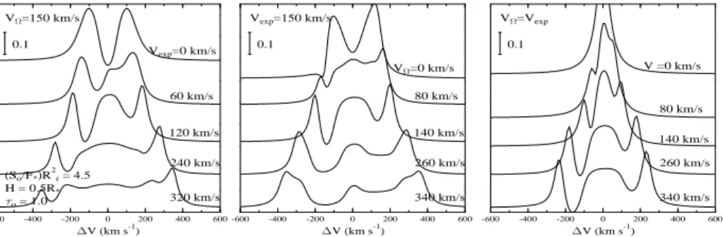
-600 -400 -200 0 200 400 600 V (km s-1) V =150 km/s o= 1.0 H = 0.5R* (So/F*)R 2 r= 4.5 Vexp=0 km/s 60 km/s 120 km/s 240 km/s 320 km/s 0.1 -600 -400 -200 0 200 400 600 V (km s-1) Vexp=150 km/s V =0 km/s 80 km/s 140 km/s 260 km/s 340 km/s 0.1 -600 -400 -200 0 200 400 600 V (km s-1) V =Vexp V =0 km/s 80 km/s 140 km/s 260 km/s 340 km/s 0.1

Figure 2. Three-peak line profiles produced by rotating+expanding rings

Φ(v) is the intrinsic absorption line profile. The line source function is: Sλ(τo) =

So for τo ≤ 1; Soτop for τo > 1 [p ≃ 1/2 for Gaussian Φ(v)] and Bλo(Te) for

τo≥ (Bλo/So)

2 _{(Mihalas 1978, Chap.11). S}

o depends on the nature of the line

transition: collision-, photoionization-, mixed-dominated. Using So as done in

Cidale & Ringuelet (1989) we can determine the excitation temperature (Arias et al. 2005). Thus, the free parameters to fit the observed emission line profiles are: So/F∗, τo, Rr, H, i, VΩ, Vexpand density distribution β (or α = 2 − β). The

shape of the line profiles reduce strongly the space of free parameters, mainly those of the velocity field and the ratio between τo and H. Line intensities

are sensitive to (So/F∗)R_r2 and Rrto the temperature, which in turn determines

So/F∗. Figure 1a shows line profiles obtained for the indicated parameters of the

ring with Vexp= 0, which are typical for ‘shell’ lines. The same ring parameters

are used for Fig. 1b, but Vexp= 150 km/s. The line profiles are of the ‘steeple’

type seen frequently in Fe ii lines. Flaring discs can be treated in the same way as cylindrical ones, except that the surface density, and hence τo depends on

the coordinate perpendicular to the equator (Vinicius et al. 2005). A fit of the Hα line of α Eri in 1994 with a flaring disc of opening angle φ = 15o is shown in Fig. 1c, where are also shown line profiles for different β-values. Several three-peak emission line profile are shown in Fig. 2 produced in regions treated

(4)

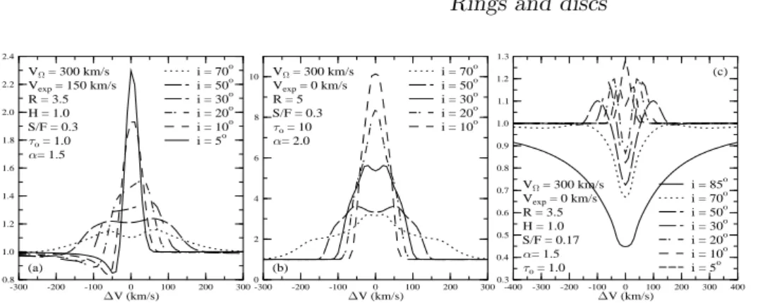
Rings and discs 3 -300 -200 -100 0 100 200 300 V (km/s) 0.8 1.0 1.2 1.4 1.6 1.8 2.0 2.2 2.4 (a) = 1.5 o= 1.0 S/F = 0.3 H = 1.0 R = 3.5 Vexp= 150 km/s V = 300 km/s i = 5o i = 10o i = 20o i = 30o i = 50o i = 70o -300 -200 -100 0 100 200 300 V (km/s) 0 2 4 6 8 10 (b) = 2.0 o= 10 S/F = 0.3 R = 5 Vexp= 0 km/s V = 300 km/s i = 10o i = 20o i = 30o i = 50o i = 70o -400 -300 -200 -100 0 100 200 300 400 V (km/s) 0.3 0.4 0.5 0.6 0.7 0.8 0.9 1.0 1.1 1.2 1.3 o= 1.0 = 1.5 S/F = 0.17 H = 1.0 R = 3.5 Vexp= 0 km/s V = 300 km/s i = 5o i = 10o i = 20o i = 30o i = 50o i = 70o i = 85o (c)

Figure 3. Emission line profiles obtained with discs. a) P Cyg like profiles. b) Bottle shaped. c) Broadening due to v1 at i → 90o

as equivalent expanding rings. Due to the Doppler shifts, the central emission components are produced by the front and rear sides of ring sectors where the radial velocity is vr≃ 0.

2. Discs

The main difference in the treatment of discs with respect to that for rings is in the velocity dependence of the intrinsic absorption line profile. It has been shown by Horne & Marsh (1986) that for a Gaussian Φ(v) the Doppler width of the profile is enlarged by a “turbulent” term due to the differential rotation in the disc towards the observer’s direction. The wavelength dependent opacity is then proportional to exp{−(1/2)[(λ − λD)/(∆D × δ)]2}, where λD= λo(vo/c) and:

vo = [VΩ(R) sin θ + Vexp(R) cos θ] sin i

δ = [1 + (λov1/c∆D)2]1/2

v1 = [1₂VΩ(R) sin θ + Vexp(R)(2 − β) cos θ] cos θ tan i sin i

  

(2)

where θ is the azimuthal angle. For large values of H, v1 acts as a non-negligible

broadening agent of the effective Doppler line width. Different examples of line profiles obtained with discs seen at several inclination angles are shown in Fig 3. The parameters used in Fig 3a can suite for P Cyg type line pro-files, while Fig 3b reproduce the bottle shaped emission line profiles seen fre-quently in Be stars. The ‘bottle’ shaped profiles can be obtained also with rings. They are produced by the τp

o opacity dependence of the source function due

to its non-local energy supply. The broadening of the effective Doppler line by v1 is depicted in Fig 3c (i = 85o). Other related subjects can be found in

http://www2.iap.fr/users/zorec/.

References

Arias, M.L. 2004, PhD Thesis, University of La Plata, Argentina Arias, M.L., Zorec, J., Cidale, L., Ringuelet, A. 2005, A&A, submitted Cidale, L.S, & Ringulete, A.E. 1989, PASP, 101, 417

Horne, K., Marsh, T.R. 1986, MNRAS, 218, 761 Mihalas, D. 1978, Stellar Atmospheres, Freeman