Detection of the Temporal Variation of the Sun's
Cosmic Ray Shadow with the IceCube Detector
The MIT Faculty has made this article openly available.
Please share
how this access benefits you. Your story matters.
Citation
Aartsen, M. G. et al. “Detection of the Temporal Variation of
the Sun’s Cosmic Ray Shadow with the IceCube Detector.” The
Astrophysical Journal 872, 2 (February 2019): 133.
As Published
http://dx.doi.org/10.3847/1538-4357/aaffd1
Publisher
IOP Publishing
Version
Final published version
Citable link
https://hdl.handle.net/1721.1/129377
Terms of Use
Article is made available in accordance with the publisher's
policy and may be subject to US copyright law. Please refer to the
publisher's site for terms of use.
Detection of the Temporal Variation of the Sun
ʼs Cosmic Ray Shadow with the IceCube
Detector
M. G. Aartsen1, M. Ackermann2, J. Adams1, J. A. Aguilar3, M. Ahlers4, M. Ahrens5, D. Altmann6, K. Andeen7, T. Anderson8, I. Ansseau3, G. Anton6, C. Argüelles9, J. Auffenberg10, S. Axani9, P. Backes10, H. Bagherpour1, X. Bai11, A. Barbano12, J. P. Barron13, S. W. Barwick14, V. Baum15, R. Bay16, J. J. Beatty17,18, J. Becker Tjus19, K.-H. Becker20, S. BenZvi21, D. Berley22, E. Bernardini2 , D. Z. Besson23, G. Binder24,16, D. Bindig20, E. Blaufuss22, S. Blot2, C. Bohm5, M. Börner25, F. Bos19, S. Böser15, O. Botner26, E. Bourbeau4, J. Bourbeau27, F. Bradascio2, J. Braun27, H.-P. Bretz2, S. Bron12, J. Brostean-Kaiser2, A. Burgman26,
R. S. Busse27, T. Carver12, C. Chen28, E. Cheung22, D. Chirkin27, K. Clark29, L. Classen30, G. H. Collin9, J. M. Conrad9, P. Coppin31, P. Correa31, D. F. Cowen8,32, R. Cross21, P. Dave28, M. Day27, J. P. A. M. de André33, C. De Clercq31, J. J. DeLaunay8, H. Dembinski34, K. Deoskar5, S. De Ridder35, P. Desiati27, K. D. de Vries31, G. de Wasseige31, M. de With36,
T. DeYoung33, J. C. Díaz-Vélez27, H. Dujmovic37, M. Dunkman8, E. Dvorak11, B. Eberhardt15, T. Ehrhardt15, B. Eichmann19, P. Eller8, P. A. Evenson34, S. Fahey27, A. R. Fazely38, J. Felde22, K. Filimonov16, C. Finley5, A. Franckowiak2, E. Friedman22,
A. Fritz15, T. K. Gaisser34, J. Gallagher39, E. Ganster10, S. Garrappa2, L. Gerhardt24, K. Ghorbani27, W. Giang13, T. Glauch40, T. Glüsenkamp6, A. Goldschmidt24, J. G. Gonzalez34, D. Grant13, Z. Griffith27, C. Haack10, A. Hallgren26, L. Halve10, F. Halzen27,
K. Hanson27, D. Hebecker36, D. Heereman3, K. Helbing20, R. Hellauer22, S. Hickford20, J. Hignight33, G. C. Hill41, K. D. Hoffman22, R. Hoffmann20, T. Hoinka25, B. Hokanson-Fasig27, K. Hoshina27,42, F. Huang8, M. Huber40 , K. Hultqvist5,
M. Hünnefeld25, R. Hussain27, S. In37, N. Iovine3, A. Ishihara43, E. Jacobi2, G. S. Japaridze44, M. Jeong37, K. Jero27, B. J. P. Jones45, P. Kalaczynski10, W. Kang37, A. Kappes30, D. Kappesser15, T. Karg2, A. Karle27, U. Katz6 , M. Kauer27, A. Keivani8, J. L. Kelley27, A. Kheirandish27 , J. Kim37, T. Kintscher2, J. Kiryluk46, T. Kittler6, S. R. Klein24,16, R. Koirala34, H. Kolanoski36, L. Köpke15, C. Kopper13, S. Kopper47, D. J. Koskinen4, M. Kowalski2,36, K. Krings40, M. Kroll19, G. Krückl15,
S. Kunwar2, N. Kurahashi48, A. Kyriacou41, M. Labare35, J. L. Lanfranchi8, M. J. Larson4, F. Lauber20, K. Leonard27, M. Leuermann10, Q. R. Liu27, E. Lohfink15, C. J. Lozano Mariscal30, L. Lu43, J. Lünemann31, W. Luszczak27, J. Madsen49, G. Maggi31, K. B. M. Mahn33, Y. Makino43, S. Mancina27, I. C. Mariş3, R. Maruyama50, K. Mase43, R. Maunu22, K. Meagher3,
M. Medici4, M. Meier25, T. Menne25, G. Merino27, T. Meures3, S. Miarecki16,24, J. Micallef33, G. Momenté15, T. Montaruli12, R. W. Moore13, M. Moulai9, R. Nagai43, R. Nahnhauer2, P. Nakarmi47, U. Naumann20, G. Neer33, H. Niederhausen46, S. C. Nowicki13, D. R. Nygren24, A. Obertacke Pollmann20, A. Olivas22, A. O’Murchadha3, E. O’Sullivan5, T. Palczewski16,24, H. Pandya34, D. V. Pankova8, P. Peiffer15, J. A. Pepper47, C. Pérez de los Heros26, D. Pieloth25, E. Pinat3, A. Pizzuto27, M. Plum7,
P. B. Price16, G. T. Przybylski24, C. Raab3, M. Rameez4, L. Rauch2, K. Rawlins51, I. C. Rea40, R. Reimann10, B. Relethford48, G. Renzi3, E. Resconi40, W. Rhode25, M. Richman48, S. Robertson24, M. Rongen10, C. Rott37, T. Ruhe25, D. Ryckbosch35, D. Rysewyk33, I. Safa27, S. E. Sanchez Herrera13, A. Sandrock25, J. Sandroos15, M. Santander47 , S. Sarkar4,52, S. Sarkar13, K. Satalecka2, M. Schaufel10, P. Schlunder25, T. Schmidt22, A. Schneider27, J. Schneider6, S. Schöneberg19, L. Schumacher10, S. Sclafani48, D. Seckel34, S. Seunarine49, J. Soedingrekso25, D. Soldin34, M. Song22, G. M. Spiczak49, C. Spiering2, J. Stachurska2,
M. Stamatikos17, T. Stanev34, A. Stasik2, R. Stein2, J. Stettner10, A. Steuer15, T. Stezelberger24, R. G. Stokstad24, A. Stößl43, N. L. Strotjohann2, T. Stuttard4, G. W. Sullivan22, M. Sutherland17, I. Taboada28, F. Tenholt19, S. Ter-Antonyan38, A. Terliuk2,
S. Tilav34, P. A. Toale47, M. N. Tobin27, C. Tönnis37, S. Toscano31, D. Tosi27, M. Tselengidou6, C. F. Tung28, A. Turcati40, R. Turcotte10, C. F. Turley8, B. Ty27, E. Unger26, M. A. Unland Elorrieta30, M. Usner2, J. Vandenbroucke27, W. Van Driessche35,
D. van Eijk27, N. van Eijndhoven31, S. Vanheule35, J. van Santen2, M. Vraeghe35, C. Walck5, A. Wallace41, M. Wallraff10, F. D. Wandler13, N. Wandkowsky27, T. B. Watson45, C. Weaver13, M. J. Weiss8, C. Wendt27, J. Werthebach27, S. Westerhoff27, B. J. Whelan41, N. Whitehorn53, K. Wiebe15, C. H. Wiebusch10, L. Wille27, D. R. Williams47, L. Wills48, M. Wolf40, J. Wood27,
T. R. Wood13, E. Woolsey13, K. Woschnagg16, G. Wrede6, D. L. Xu27, X. W. Xu38, Y. Xu46, J. P. Yanez13, G. Yodh14, S. Yoshida43, and T. Yuan27
IceCube Collaboration 1
Dept. of Physics and Astronomy, University of Canterbury, Private Bag 4800, Christchurch, New Zealand;analysis@icecube.wisc.edu
2DESY, D-15738 Zeuthen, Germany 3
Université Libre de Bruxelles, Science Faculty CP230, B-1050 Brussels, Belgium
4
Niels Bohr Institute, University of Copenhagen, DK-2100 Copenhagen, Denmark
5
Oskar Klein Centre and Dept. of Physics, Stockholm University, SE-10691 Stockholm, Sweden
6
Erlangen Centre for Astroparticle Physics, Friedrich-Alexander-Universität Erlangen-Nürnberg, D-91058 Erlangen, Germany
7
Department of Physics, Marquette University, Milwaukee, WI 53201, USA
8
Dept. of Physics, Pennsylvania State University, University Park, PA 16802, USA
9
Dept. of Physics, Massachusetts Institute of Technology, Cambridge, MA 02139, USA
10
III. Physikalisches Institut, RWTH Aachen University, D-52056 Aachen, Germany
11
Physics Department, South Dakota School of Mines and Technology, Rapid City, SD 57701, USA
12
Département de physique nucléaire et corpusculaire, Université de Genève, CH-1211 Genève, Switzerland
13Dept. of Physics, University of Alberta, Edmonton, Alberta T6G 2E1, Canada 14
Dept. of Physics and Astronomy, University of California, Irvine, CA 92697, USA
15
Institute of Physics, University of Mainz, Staudinger Weg 7, D-55099 Mainz, Germany
16
Dept. of Physics, University of California, Berkeley, CA 94720, USA
17Dept. of Physics and Center for Cosmology and Astro-Particle Physics, Ohio State University, Columbus, OH 43210, USA 18
Dept. of Astronomy, Ohio State University, Columbus, OH 43210, USA
19
Fakultät für Physik & Astronomie, Ruhr-Universität Bochum, D-44780 Bochum, Germany
20
Dept. of Physics, University of Wuppertal, D-42119 Wuppertal, Germany
21
Dept. of Physics and Astronomy, University of Rochester, Rochester, NY 14627, USA
22
Dept. of Physics, University of Maryland, College Park, MD 20742, USA
23
Dept. of Physics and Astronomy, University of Kansas, Lawrence, KS 66045, USA
24
Lawrence Berkeley National Laboratory, Berkeley, CA 94720, USA
25
Dept. of Physics, TU Dortmund University, D-44221 Dortmund, Germany
26Dept. of Physics and Astronomy, Uppsala University, Box 516, SE-75120 Uppsala, Sweden 27
Dept. of Physics and Wisconsin IceCube Particle Astrophysics Center, University of Wisconsin, Madison, WI 53706, USA
28
School of Physics and Center for Relativistic Astrophysics, Georgia Institute of Technology, Atlanta, GA 30332, USA
29
SNOLAB, 1039 Regional Road 24, Creighton Mine 9, Lively, ON P3Y 1N2, Canada
30
Institut für Kernphysik, Westfälische Wilhelms-Universität Münster, D-48149 Münster, Germany
31
Vrije Universiteit Brussel(VUB), Dienst ELEM, B-1050 Brussels, Belgium
32
Dept. of Astronomy and Astrophysics, Pennsylvania State University, University Park, PA 16802, USA
33
Dept. of Physics and Astronomy, Michigan State University, East Lansing, MI 48824, USA
34
Bartol Research Institute and Dept. of Physics and Astronomy, University of Delaware, Newark, DE 19716, USA
35
Dept. of Physics and Astronomy, University of Gent, B-9000 Gent, Belgium
36
Institut für Physik, Humboldt-Universität zu Berlin, D-12489 Berlin, Germany
37
Dept. of Physics, Sungkyunkwan University, Suwon 440-746, Republic of Korea
38
Dept. of Physics, Southern University, Baton Rouge, LA 70813, USA
39
Dept. of Astronomy, University of Wisconsin, Madison, WI 53706, USA
40
Physik-department, Technische Universität München, D-85748 Garching, Germany
41
Department of Physics, University of Adelaide, Adelaide, 5005, Australia
42
Earthquake Research Institute, University of Tokyo, Bunkyo, Tokyo 113-0032, Japan
43
Dept. of Physics and Institute for Global Prominent Research, Chiba University, Chiba 263-8522, Japan
44
CTSPS, Clark-Atlanta University, Atlanta, GA 30314, USA
45
Dept. of Physics, University of Texas at Arlington, 502 Yates St., Science Hall Rm 108, Box 19059, Arlington, TX 76019, USA
46
Dept. of Physics and Astronomy, Stony Brook University, Stony Brook, NY 11794-3800, USA
47
Dept. of Physics and Astronomy, University of Alabama, Tuscaloosa, AL 35487, USA
48
Dept. of Physics, Drexel University, 3141 Chestnut Street, Philadelphia, PA 19104, USA
49
Dept. of Physics, University of Wisconsin, River Falls, WI 54022, USA
50
Dept. of Physics, Yale University, New Haven, CT 06520, USA
51
Dept. of Physics and Astronomy, University of Alaska Anchorage, 3211 Providence Dr., Anchorage, AK 99508, USA
52
Dept. of Physics, University of Oxford, 1 Keble Road, Oxford OX1 3NP, UK
53
Department of Physics and Astronomy, UCLA, Los Angeles, CA 90095, USA
Received 2018 November 6; revised 2019 January 14; accepted 2019 January 16; published 2019 February 19
Abstract
We report on the observation of a deficit in the cosmic ray flux from the directions of the Moon and Sun with five years of data taken by the IceCube Neutrino Observatory. Between 2010 May and 2011 May the IceCube detector operated with 79 strings deployed in the glacial ice at the South Pole, and with 86 strings between 2011 May and 2015 May. A binned analysis is used to measure the relative deficit and significance of the cosmic ray shadows. Both the cosmic ray Moon and Sun shadows are detected with high statistical significance (>10σ) for each year. The results for the Moon shadow are consistent with previous analyses and verify the stability of the IceCube detector over time. This work represents thefirst observation of the Sun shadow with the IceCube detector. We show that the cosmic ray shadow of the Sun varies with time. These results make it possible to study cosmic ray transport near the Sun with future data from IceCube.
Key words: cosmic rays – ISM: magnetic fields – Moon – Sun: activity – sunspots 1. Introduction
The IceCube Neutrino Observatory (Aartsen et al. 2017) comprises a 1 km3 Cerenkov light detector buried in the Antarctic ice between 1450 and 2450 m below the geographic South Pole. The trigger rate is dominated by atmospheric muons that are produced when cosmic ray particles interact with the Earth’s atmosphere. Cosmic rays from the direction of the Moon and Sun are absorbed by the celestial bodies. The deficit in the cosmic ray flux toward the direction of the Moon was already observed by IceCube with its 40 and 59 string configurations, using data collected from 2008 May to 2010 May. Two independent analyses observed the deficit in the cosmic ray flux with high statistical significance (>6σ) (Aartsen et al.2014).
The main purpose of the previous paper was to verify the pointing of the detector. In this paper, we investigate for the
first time the Sun shadow as well. Here, the goal is to study the temporal behavior of the two shadows: while the Moon is expected to be stable in time (with only smaller variations expected due to the changing apparent size), the Sun shadow has been shown to vary with the solar cycle and, in turn, with the Sun’s magnetic field (Amenomori et al.2013), and has been used to measure the mean interplanetary magneticfield (Aielli et al. 2011). It is the goal of this analysis to investigate whetherthe effect of a temporal variation is present even at the high energies that IceCube is sensitive to (median primary particle energy of events passing the Moon and Sun filters: ∼40 TeV, see Section2.3).
IceCube detects cosmic rays via high-energy secondary muons, which are produced when cosmic ray particles interact with the Earth’s atmosphere. The Moon and the Sun subtend an angle of ∼0°.5, which is smaller than the median angular
resolution for muon detection. The Moon can be used to estimate the resolution and pointing in IceCube. Other experiments have also used the Moon as a calibrator to measure the angular resolution and absolute pointing capabil-ities of their detectors(see Ambrosio et al.2003; Achard et al. 2005; Oshima et al. 2010; Adamson et al.2011; Bartoli et al. 2011; Abeysekara et al. 2013). However, the Sun cannot be used to calibrate the IceCube detector as the solar magnetic field is expected to influence cosmic rays on their way to Earth. The Tibet-AS Gamma experiment analyzed the cosmic ray shadow caused by the Sun (median primary particle energy: ∼10 TeV) and discovered an influence of the solar magnetic field, presented in Amenomori et al. (2013). The depth of the Sun shadow varied during the observation period from 1996 through 2009, while the cosmic ray shadow of the Moon was measured to be constant over time within the experimental uncertainties in Amenomori et al. (2013), as expected. Tibet finds that the variation can be well described by including cosmic ray transport in the solar magnetic field.
It is the aim of this paper to use IceCube data to provide an independent observation of the temporal variation of the Sun shadow. In addition, IceCube measures particles at a mean energy of around 40TeV, which is at significantly higher energies as compared to Tibet. Establishing the measurement of the cosmic ray shadow of the Sun with IceCube and other experiments will provide long-term energy-dependent informa-tion on the cosmic ray transport in the solar magnetic field, which makes this study particularly interesting.
The IceCube cosmic ray Moon and Sun shadow analysis is based on a binned analysis that measures the relative deficit of events from the direction of the celestial bodies. Additionally, a two-dimensional visualization of the shadow is derived. Both methods make use of data from on- and off-source regions with events taken from the same elevation as the Moon and Sun but at different R.A. This is possible due to IceCube’s uniform exposure in R.A.
2. Detector Configuration and Data Sample 2.1. IceCube Detector
The IceCube Neutrino Observatory comprises two compo-nents: the IceCube neutrino telescope, which detects penetrat-ing muons and neutrinos, and the IceTop surface array, which detects extensive air showers induced by high-energy cosmic rays. The IceCube neutrino telescope makes use of the glacial ice as a detection medium for the Cerenkov radiation from charged particles. Charged relativistic particles emit Cerenkov light in media, where the speed of light is reduced by the index of refraction. IceCube consists of 5160 Digital Optical Modules (DOMs) arranged on 86 vertical cables (called strings). Each DOM contains a 10 inch photomultiplier tube enclosed in a glass pressure sphere.
IceCube’s primary goal is to detect high-energy neutrinos from astrophysical sources; see, e.g., Halzen & Klein (2010) and Becker(2008) for reviews. Cosmic-ray-induced muons and neutrinos from the atmosphere, which are a background for astrophysical neutrino searches, are far more abundant and comprise most IceCube triggers. These cosmic ray events can be used to investigate particle interaction physics in the forward direction, to study cosmic rays themselves, or to trace back cosmic ray directions as in this work. In this analysis, atmospheric muons are used to investigate the shadow in the
cosmic ray flux caused by the Sun and the Moon. As the detected muons are highly relativistic, the direction of the cosmic ray can be derived from the muon’s direction. Estimating the average primary cosmic ray energy of the sample is also possible through comparison to simulations.
During 2010 May and 2011 May IceCube detected high-energy particles with 79 strings(IC79) before it operated in its final detector configuration with 86 strings (IC86). In this paper, data were taken from the IC79 and four years IC86 (I–IV) configuration. A sketch of the final detector configura-tion can be seen in Figure1.
2.2. Data Sample
Down-going muons, with an energy of roughly more than 400 GeV, dominate the total trigger rate of 2100 s−1 (Aartsen et al.2017). Due to limited data transfer bandwidth of 100 GB per day from the South Pole to the Northern Hemisphere, onlinefilters are used to reduce the amount of data. This paper uses filtered data streams specifically designed to study the Moon and Sun shadows. These filters are angular windows (±10° in zenith, ±180° in azimuth) around the expected position of Moon and Sun, and are enabled when at least 12 DOMs in three different strings detect photons. Furthermore, the Moon and Sun have to reach at least an elevation of 15° above the horizon to satisfy the online filters. Quality cuts improving the directional reconstruction are applied to all events passing thesefilters (see Section2.4). The Sun reaches a maximum elevation of ∼23°.5 each year, while the Moon’s maximum elevation varies between ∼24° and ∼18° at the geographic South Pole for the fraction of the lunar nodal precession covered by these observations. The Moon filter is enabled for several consecutive days each month, whereas the Sun filter collects data for approximately 90 days from November through February each season.
At the South Pole, a fast likelihood-based track reconstruc-tion(Ahrens et al.2004) is performed for each muon event and its direction is compared to the expected position of the celestial body in angular coordinates. The data are transferred to the Northern Hemisphere by satellite if the reconstructed event satisfies the Moon or Sun filter. Offline, after the events
Figure 1.Sketch of the IceCube Neutrino Observatory in itsfinal detector configuration. A more compact group of Digital Optical Modules, named DeepCore, is located at the bottom of the detector. Also shown is IceTop, a surface cosmic ray detector, which consists of 162 water Cerenkov tanks with 324 optical sensors. IceTop data are not used in this work.
have been transferred, a more sophisticated reconstruction chain is applied. The direction of each event is reconstructed using a method similar to that described in Aartsen et al. (2014), only instead of a single-photoelectron fit, a multi-photoelectron fit is performed which uses timing information from all photons rather than just thefirst photons to arrive. The angular uncertainty sigma of the reconstructed direction is computed by thenfitting a paraboloid to the likelihood around its minimum andfinding the size of the 1σ ellipsoidal contour; see Neunhöffer(2006) for more details.
2.3. Simulations
Simulations are used to verify experimental data, e.g., the zenith angle distribution, and to optimize the used quality cuts (see Section 2.4). This paper makes use of CORSIKA simulations with a primary energy range from 600 GeV to 1011GeV and five mass components (p, He, N, Al, Fe). CORSIKA is a Monte Carlo-based code that simulates extensive air showers which are produced when cosmic ray particles interact with Earth’s atmosphere (Heck et al. 1998). This work uses the high-energy hadronic interaction model Sibyll 2.1 (Ahn et al. 2009) and the Antarctic atmospheric profile according to the MSIS-90-E model. The CORSIKA sample is weighted with the Gaisser H3a model from Gaisser (2012) and compared to the data of the Moon and Sun shadow. The simulation sample that triggers the IceCube detector and satisfies the Moon and Sun filters has a median primary particle energy of 40 TeV. For 68% of the events in the sample, the energy of the primary particle is between 11 and 200 TeV. The CORSIKA generated events are fed into a full detector simulation. The same filtering and processing as for exper-imental data is used. For a more detailed description of the simulations, see Bos(2017).
2.4. Quality Cuts
Events which are mis-reconstructed or have poor angular resolution would reduce the sensitivity of the analysis described in Section 3. Quality cuts are used to remove these events. The analysis makes use of two cut variables: the angular uncertainty σ of the reconstructed event and a track reconstruction quality estimator, the reduced log-likelihood (rlogl). Both cut variables are typically used in point-source and other IceCube analyses (Abbasi et al. 2011). Assuming Poisson statistics, the significance S˜ of the shadowing effect is proportional to the square root of the fraction η of events passing the cuts and the resulting median angular resolution σmedafter the cuts(Aartsen et al.2014), (Bos et al.2015):
S . 1 med h s µ ˜ ( )
For both IC79 and IC86 the quality cuts are optimized in order to maximize the significance S˜, and the resulting optimal cut values are σ<0°.71 and rlogl<8.1 (Bos et al. 2015). In an angular window with a size of [72×16]° in R.A. and decl. around the position of the Moon and Sun, 15–24 million events for the Moon and 40–48 million events for the Sun pass the quality cuts of the analysis each year. The number of events that are used in the Moon shadow analysis varies because of the change of the maximum elevation of the Moon each year. At higher elevations more muons reach the IceCube detector.
3. Binned Analysis
A one-dimensional binned analysis of the Moon and Sun shadows is used to study their depth and to estimate the angular resolution of the event reconstruction. The analysis observes a profile view of the Moon and Sun shadow and computes the relative deficit of muon events. A two-dimensional binned approach uses maps in R.A. and decl. to show the shape of the shadows.
3.1. One-dimensional Approach 3.1.1. Description of the Method
The main goal of the 1D analysis is to observe the profile view of the Moon and Sun shadow and to estimate the angular resolution of IceCube with respect to the studied sample of high-energy muons. To measure the deficit in the cosmic ray flux from the direction of the celestial bodies, on- and off-source windows are compared in bins of radial distanceΨ to the Moon/ Sun. The on-source windows are centered around the expected positions of the Moon and the Sun and have a size of±5°. The off-source regions are eight windows of the same size with an offset of ±5°, ±10°, ±15° and ±20° from the expected positions of the Moon and the Sun in R.A. Because the number of events increases with decl., it is important that the off-source regions have an offset only in R.A. Then, the number of events in each bin in the on-source region is compared with the average number of events in each bin in the eight off-source regions.
The relative deficit between the number of events in the ith bin in the on-source region and the average number of events in the same bin in the eight off-source regions is described by
N N N N N , 2 i i i i i on off off D á ñ = - á ñ á ñ ( )
with Non off being the number of events in on-source/ off-source regions. The uncertainty is given by
N N N s N 1 1 . 3 N N i i i i on off on off i i s = á ñ + á ñ D á ñ · ( )
Here, s=8 is the number of off-source regions that are compared with the on-source region. In Aartsen et al.(2014) and Bos et al.(2015) the Moon is expected to be a point-like cosmic ray sink which reduces the muon sample byFpRM2 events. Here, Φ is the cosmic ray flux at the location of the Moon. The same
Table 1
Results of the One-dimensional Analysis, with A as the Amplitude and σμas
the Width of the Gaussian
Year σμ(°) A S(σ) 2010/11 0.43±0.05 0.12±0.02 >12 2011/12 0.45±0.05 0.13±0.02 >13 Moon 2012/13 0.49±0.05 0.11±0.02 >12 2013/14 0.47±0.05 0.12±0.02 >12 2014/15 0.47±0.06 0.13±0.02 >11 2010/11 0.53±0.05 0.11±0.01 >16 2011/12 0.49±0.06 0.08±0.01 >13 Sun 2012/13 0.57±0.05 0.09±0.01 >16 2013/14 0.58±0.07 0.05±0.01 >10 2014/15 0.57±0.07 0.06±0.01 >10
approach is used in this paper. Here, the radii of the Moon and Sun are described as RM/S≈0°.26. The exact apparent size of
the Moon and Sun depends on their distance from Earth and varies between 0°.24 and 0°.28. The relative deficit is smeared by the point-spread function (PSF) of the IceCube detector. Under the assumption that the PSF is approximately described by an azimuthally symmetric Gaussian function, it only depends on the radial distanceΨ and is given by Aartsen et al. (2014) as
f RM S e . 4 2 2 2 2 2 p s Y = -F m s -Y m ( ) · ( )
Here,σμis the angular resolution of the studied muon sample. The relative deficit in the ith bin is
N N R e 2 . 5 i i i M S 2 2 2 i 2 2 s D á ñ Y = - m s -Y m ( ) ( )
Equation (5) is fitted to IceCube’s experimental data. The amplitude A R 2 6 M S 2 2 s = m ( ) and the angular resolutionσμare free parameters of thefit.
We studied the influence of the above fitting procedure on a disk-like sink of cosmic rays(hence, atmospheric muons) that is smeared by a more realistic PSF of the detector as obtained from the simulations described in Section 2.3. That PSF deviates considerably from the Gaussian approximation made above, especially in the region of large angular errors. As a result, inferring the radius RM/Sfrom thefit parameters A and
σμusing Equation(6) induces a bias toward smaller radii, and
Equation(6) cannot be used to infer the geometrical radii of the Moon or Sun.
Moreover, as in Aartsen et al.(2014), the angular size of the Moon and Sun is ignored, which can affect the results of thefit.
Figure 2.Observed cosmic ray deficit due to the Moon shadow inferred with the binned analysis in one dimension. The relative deficit in the number of events in on-source and off-on-source regions of each bin is shown for each year as a function of the radial distanceΨ to the Moon. The amplitude A and the width σμremain constant,
Due to the angular resolution of the IceCube detector, which is on the order of 0°.5, the influence of the angular size of the Moon and Sun should be a few percent at most(Aartsen et al.2014). By comparing the χ2 of the data points with respect to a constant linecconst2 , which illustrates the relative deficit without considering any shadowing effects (which is equivalent to assuming aflat background), and thecGaussian2 of the data points with respect to thefitted Gaussian, the statistical significance is computed: ndof ndof , 7 2 Gaussian 2 const 2 c c c D D = -D ( )
where Δndof is the difference of the number of degrees of freedom between the flat model and the Gaussian model. Calculating the p-value via Δχ2results in the significance S:
S= 2 ·erf-1(1-p). ( )8
3.1.2. Results
After the quality cuts are applied to IceCube’s experimental data, approximately 30% of all muon events passing Moon and Sunfilters survive these cuts each year and are used to analyze the cosmic ray Moon and Sun shadow. Results for the 1D analysis can be found in Table 1. Keep in mind that for the reasons described in Section3.1.1thefit parameters A and σμ in Table 1 cannot be used to infer the geometrical radii of Moon and Sun.
The cosmic ray Moon shadow is observed with high statistical significance (>11σ) in every year. The angular resolution of the Moon shadow analysis, given by the width of the fitted Gaussian, remains stable for the entire observation period. IceCube’s median angular error σmed, as derived from
simulations, is 0°.68, and 68% of the events are contained between 0°.29 and 1°.62. The data analysis shows better angular resolution compared to the median angular error, which is expected and was already observed in Aartsen et al.(2014).
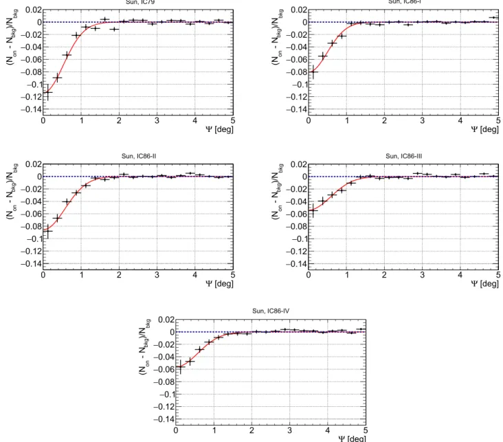
Figure 3.Observed cosmic ray deficit due to the Sun shadow inferred with the binned analysis in one-dimension. The relative deficit in the number of events in on-source and off-on-source regions of each bin is shown for each year as a function of the radial distanceΨ to the Sun. The amplitude varies during the five year observation time.
Figure 4.Results for the binned visualization of the Moon shadow in two dimensions. The expected position of the Moon is in the middle of the[6°×6°] plot. The black circle shows the actual size of the Moon. A smoothing radius has a size of 0°.35. Each map shows the cosmic ray Moon shadow for a season from 2010 through 2015. The contour represents the relative deficit of events in each bin. The shadowing remains stable for the entire observation period, which is expected for a stably operating detector.
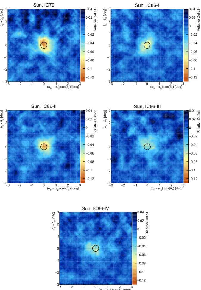
Figure 5.Seasonal results for the 2D binned maps of the Sun shadow. Each map uses data from November through February of each season. In IC79 the shadowing effect of the Sun is similar to the Moon shadow. Variations are clearly visible during IC86 I–IV (2011–2015) and are quantified in this paper (see the text).
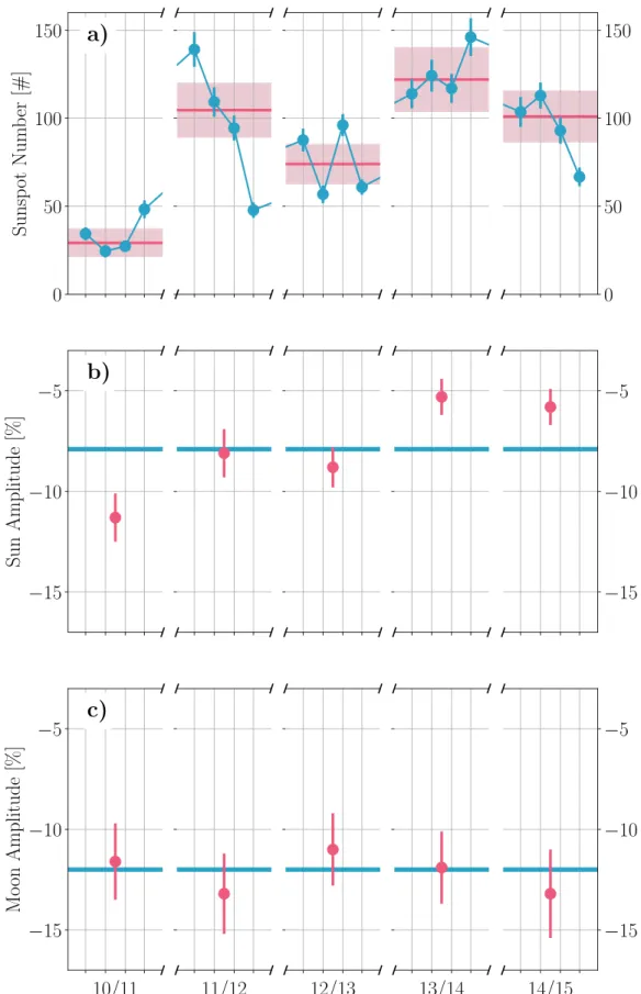
Figure 6.Comparing the solar activity with IceCube’s cosmic ray Moon and Sun shadow analysis. (a) Monthly mean sunspot number in November, December, January, and February of each year. The red line shows the weighted mean of the sunspot number for each year.(b) Measured amplitude in the one-dimensional analysis for the Sun shadow using data. The blue line shows the mean amplitude across thefive years of data. (c) Measured amplitude in the one-dimensional analysis for the Moon shadow using data. The blue line shows the mean amplitude across thefive years of data without a modulation due to changes in the apparent size of the Moon which here amounts to about±0.5%. Sunspot numbers are taken from SILSO World Data Center (2016).
Furthermore, the amplitude varies only within its statistical uncertainties. These results show that the IceCube detector is operating stably for thefive year observation period. In Aartsen et al. (2014), where data are used from two years in which IceCube operated in smaller detector configurations, the median angular resolution was measured to be(0.71±0.07)° and (0.63±0.04)° for the 40 string configuration in 2008/ 2009 and the 59 string configuration in 2009/2010, respec-tively. The differences between IC 40, IC 59 and this analysis are expected, because this work makes use of thefinal detector configuration with 86 strings and the previous configuration with 79 strings.
In Figure2the 1D analysis results for the Moon shadow are shown for the five year observation period. The y-axis illustrates the relative deficit of events in each bin of the on-source and off-on-source regions as a function of the angular distance on the x-axis. A Gaussian (red line) with parameters from Table 1 and a line for no relative deficit (blue line) are also shown.
The 1D analysis is performed for the Sun shadow analysis for the same observation period (see Table 1). As we derive quantitatively from the width and amplitude of the shadow(see Table 1), the angular resolution is consistent with a constant value for thefive year observation period. The amplitude of the Sun shadow, on the other hand, varies between(11±1)% and (5±1)%. For the Sun, the interpretation of A and σμis more
complex than for the Moon. Besides the detector effects that cause the smearing in the case of the Moon shadow, we also expect physical solar effects to be relevant in the case of the Sun shadow. For example, the deflection of cosmic rays in the solar magnetic field can presumably change the values measured for A and σμ. In this paper, we do not aim to
separate the effects of absorption and deflection on the Sun shadow. The time variability of A that can be seen in Table1, however, must be intrinsic to the Sun since for the Moon both fit parameters remain stable during the observation period. Figure3shows the measured one-dimensional Sun shadow for each of the five years.
3.2. Two-dimensional Approach 3.2.1. Description of the Method
In a second approach, two-dimensional maps of the cosmic ray shadows of the Moon and Sun are created. The goal is to make the shadowing effects of the Moon and Sun visible in a three-dimensional representation, with the magnitude of the shadowing effect as the third dimension. This approach compares each bin of an on-source region with the average of the same bins of two off-source regions with an offset of ±18° in R.A. Due to a higher muon trigger rate from higher decl., the off-source regions only have an offset in R.A. A map with a size of [6°×6°] around the expected position of the celestial bodies is used to show relative decl., relative R.A. and relative deficit of events in each bin.
After assigning muon events to on- and off-source regions, a smoothing method, which takes the average number of events within a chosen rebinning radius of 0°.35 of each bin in the [6°×6°] window, is applied in order to make the shadowing effects visible. In order to maximize the statistical significance, a bigger rebinning radius can be used. However, the goal of this approach is to show the shadowing effects of Moon and Sun with the highest relative deficit. Thus, the rebinning radius is chosen to be smaller than the angular size of Moon and Sun. With a rebinning radius of 0°.35 the lower limit is reached. Smaller radii would lead to shadowing effects with insufficient statistical significance. Similar methods to analyze the shadowing effects of the Moon and Sun are used in, e.g., Abeysekara et al.(2013) and Amenomori et al. (2013).
3.2.2. Results
Figure4shows the results of the two-dimensional approach for the IC79 and four years of the IC86 (I–IV) configuration. The black circle illustrates the actual size of the Moon of 0°.5. The Moon shadow remains almost stable for the entirefive year observation period, which confirms stable operation of the detector. This result is consistent with the binned analysis in one dimension(Table 1).
Figure 7.Measured amplitude in the one-dimensional analysis for the Sun shadow as a function of the weighted average monthly sunspot number. A Spearman’s rank correlation gives a hint of a correlation with a p-value of 96%. Sunspot numbers are taken from SILSO World Data Center (2016).
The calculated center for the position of the Moon shadow is located in the middle of the map, which also represents the expected position of the Moon. However, this method is only an estimator for the position of the Moon. A more sophisticated unbinned likelihood method to analyze the pointing accuracy of IceCube, given the known position of the Moon, is performed in Aartsen et al.(2014).
The results for the two-dimensional binned approach of the Sun shadow can be seen in Figure5. Compared with the Moon shadow, the Sun shadow varies during the observation time, which confirms the results obtained in the 1D analysis. A similar effect is observed in Zhu (2016) for data from 2008 through 2012 and in Amenomori et al.(2013). In Amenomori et al. it is shown that in thefirst year (2010/11) the shadowing effect is similar to the Moon shadow. The shadowing effect decreases in 2011/12 and increases in 2012/13. The weakest shadowing effect can be seen in 2013/14 and 2014/15. The next section will compare the measured Sun shadow with the solar activity.
4. Solar Activity
The Sun has a magnetic field that varies over a 22 year cycle and displays magnetic activity in cycles of about 11 years. A direct estimator for the solar activity is the sunspot number. Cosmic ray particles are expected to be influenced by the solar magnetic field on their way to Earth. The binned analysis shows a constant Moon shadow and a time-variable Sun shadow. IceCube records data from the direction of the Sun from November through February each year. Due to the solar cycle, the solar activity changes for each season. A minimum of the monthly average sunspot number is observed with 24.5±3.6 in 2010 December, a maximum with 146.1±10.7 in 2014 February by SILSO World Data Center (2016).
Figure6 shows a comparison of the amplitude of the fitted Gaussian in the binned 1D analysis and the sunspot number from SILSO World Data Center (2016). The first plot (a) in Figure6shows the weighted average sunspot number for each observation period, illustrated by the red line and the band as the statistical variation. Each monthly average sunspot number is weighted by the number of muon events in that particular month contributing to the final event sample of the corresp-onding observation period. The monthly average sunspot num-bers are represented by the blue data points. In (b) the amplitude of thefitted Gaussian of the Sun shadow analysis is shown by the red data points for each of the five detector configurations. The mean amplitude of the Sun shadow (blue line) is shown as a comparison. The mean amplitude of the Sun shadow data analysis is computed as (7.9±0.5)%. The deviation of these five data points from the mean amplitude can be quantified by χ2/ndof=22.47/4, which results in a statistical significance of 3.8σ. We conclude that there is a significant deviation from the mean shadowing effect of the Sun. A Spearman’s rank correlation gives a hint to a correlation between the sunspot number and the amplitude of the Gaussian (compare Figure 7) with a p-value of 96%. However, this correlation needs to be studied further, due to a weak solar cycle and the small number of observed Sun periods at this point. The third plot(c) of Figure6shows the amplitude of the Moon shadow analysis from Table 1. Here, the amplitude remains stable around its mean value (12.2±0.9)%. These
results show that the Moon shadow remains stable and can be used as a verification tool for the Sun shadow analysis.
5. Conclusion
The shadowing effects of Moon and Sun are observed with high statistical significance (>10σ) with the IceCube detector for every one year data set, with data taken from its 79 and 86 string configurations in a five year observation period. These results can be compared with the Moon shadow analyses of previous detector configurations where the existence of the shadowing effect was shown at a level of>6σ significance (Aartsen et al.2014).
This analysis, using 79 and 86 strings, achieves higher significance than the previous analysis, which had only 40 and 59 strings available. Using a binned analysis, a stable shadowing effect of the Moon is measured for the entirefive year period. This shows that the IceCube detector operates stably. The stable shadowing of the Moon also suggests that the magnetic fields between Earth and the Moon do not significantly influence cosmic rays at the energies of this analysis. However, the cosmic ray Sun shadow varies for each season.
A significant difference between IceCube’s measured Sun shadow and the mean shadowing effect of the Sun was determined as χ2/ndof=22.47/4 resulting in a statistical significance of 3.8σ. This suggests that the shadow is not constant in time. An obvious explanation would be a variation with the Sun’s magnetic field, as was also detected during the previous solar cycle at lower energies by Tibet (Amenomori et al. 2013). A Spearman’s rank correlation test shows that a correlation between the sunspot number and the amplitude of the Gaussian in the Sun shadow analysis is likely with 96%.
However, due to the low number of observation periods in combination with a relatively weak solar cycle, this correlation must be investigated further. Additional observation seasons are necessary to verify the correlation between the solar activity and the shadowing effect of the Sun. Future analyses, including the deflection of cosmic rays due to magnetic fields between the Sun and Earth, should include a more complex treatment of the PSF in order to compare results from data and simulations with respect to the integrated depth of the shadows.
USA—U.S. National Science Foundation-Office of Polar Programs, U.S. National Science Foundation-Physics Division, Wisconsin Alumni Research Foundation, Center for High Throughput Computing (CHTC) at the University of Wiscon-sin-Madison, Open Science Grid (OSG), Extreme Science and Engineering Discovery Environment (XSEDE), U.S. Depart-ment of Energy-National Energy Research Scientific Computing Center, Particle astrophysics research computing center at the University of Maryland, Institute for Cyber-Enabled Research at Michigan State University, and Astroparticle physics computa-tional facility at Marquette University; Belgium—Funds for Scientific Research (FRS-FNRS and FWO), FWO Odysseus and Big Science programmes, and Belgian Federal Science Policy Office (Belspo); Germany—Bundesministerium für Bildung und Forschung(BMBF), Deutsche Forschungsgemeinschaft (DFG), Helmholtz Alliance for Astroparticle Physics(HAP), Initiative and Networking Fund of the Helmholtz Association, Deutsches Elektronen Synchrotron (DESY), and High Performance Computing cluster of the RWTH Aachen; Sweden—Swedish Research Council, Swedish Polar Research Secretariat, Swedish
National Infrastructure for Computing (SNIC), and Knut and Alice Wallenberg Foundation; Australia—Australian Research Council; Canada—Natural Sciences and Engineering Research Council of Canada, Calcul Québec, Compute Ontario, Canada Foundation for Innovation, WestGrid, and Compute Canada; Denmark—Villum Fonden, Danish National Research Founda-tion (DNRF), Carlsberg Foundation; New Zealand—Marsden Fund; Japan—Japan Society for Promotion of Science (JSPS) and Institute for Global Prominent Research (IGPR) of Chiba University; Korea—National Research Foundation of Korea (NRF); Switzerland—Swiss National Science Foundation (SNSF). The IceCube collaboration acknowledges the significant contributions to this manuscript from Fabian Bos and Frederik Tenholt. ORCID iDs E. Bernardini https://orcid.org/0000-0003-3108-1141 M. Huber https://orcid.org/0000-0003-1059-9603 U. Katz https://orcid.org/0000-0002-7063-4418 A. Kheirandish https: //orcid.org/0000-0001-7074-0539 M. Santander https://orcid.org/0000-0001-7297-8217 References
Aartsen, M., Abbasi, R., Abdou, Y., et al. 2014,PhRvD,89, 102004
Aartsen, M. G., Ackermann, M., Adams, J., et al. 2017,JInst,12, P03012
Abbasi, R., Abdou, Y., Abu-Zayyad, T., et al. 2011,ApJ,732, 18
Abeysekara, A., Alfaro, R., Alvarez, C., et al. 2013, arXiv:1310.0072
Achard, P., Adriani, O., Aguilar-Benitez, M., et al. 2005,APh,23, 411
Adamson, P., Andreopolous, C., Ayres, D. S., et al. 2011,APh,34, 457
Ahn, E.-J., Engel, R., Gaisser, T. K., Lipari, P., & Stanev, T. 2009,PhRvD,80, 094003
Ahrens, J., Bai, X., Bay, R., et al. 2004,NucIM, A524, 169 Aielli, G., Bacci, C., Bartoli, B., et al. 2011,ApJ,729, 113
Ambrosio, M., Antolini, R., Baldini, A., et al. 2003,APh,20, 145
Amenomori, M., Bi, X. J., Chen, D., et al. 2013,PhRvL,111, 011101
Bartoli, B., Bernadini, P., Bi, X. J., et al. 2011,PhRvD,84, 022003
Becker, J. K. 2008,PhR,458, 173
Bos, F. 2017, PhD thesis, Ruhr-Universität Bochum, Universitätsbibliothek Bos, F., Tenholt, F., Becker Tjus, J., & Westerhoff, S. 2015,ASTRP,2, 5
Gaisser, T. K. 2012,APh,35, 801
Halzen, F., & Klein, S. R. 2010,RScI,81, 081101
Heck, D., Knapp, J., Capdevielle, J. N., Schatz, G., & Thouw, T. 1998, Tech. Rep. FZKA 6019(Hannover: TIB)
Neunhöffer, T. 2006,APh,25, 220
Oshima, A., Dugad, S. R., Goswami, U. D., et al. 2010,APh,33, 97
SILSO World Data Center 2016, International sunspot Number Monthly Bulletin and Online Catalogue


![Figure 4. Results for the binned visualization of the Moon shadow in two dimensions. The expected position of the Moon is in the middle of the [ 6 °× 6 °] plot](https://thumb-eu.123doks.com/thumbv2/123doknet/14724971.571488/8.918.113.808.68.1064/figure-results-binned-visualization-shadow-dimensions-expected-position.webp)