Geometry Textures

HAL Id: inria-00186866

https://hal.inria.fr/inria-00186866

Submitted on 12 Nov 2007

HAL is a multi-disciplinary open access

archive for the deposit and dissemination of

sci-entific research documents, whether they are

pub-lished or not. The documents may come from

teaching and research institutions in France or

abroad, or from public or private research centers.

L’archive ouverte pluridisciplinaire HAL, est

destinée au dépôt et à la diffusion de documents

scientifiques de niveau recherche, publiés ou non,

émanant des établissements d’enseignement et de

recherche français ou étrangers, des laboratoires

publics ou privés.

Geometry Textures

Rodrigo Toledo, Bin Wang, Bruno Lévy

To cite this version:

Rodrigo Toledo, Bin Wang, Bruno Lévy. Geometry Textures. 20th Brazilian Symposium on

Com-puter Graphics and Image Processing - SIBGRAPI 2007, Oct 2007, Belo Horizonte, Brazil. pp.79-86,

�10.1109/SIBGRA.2007.4368171�. �inria-00186866�

Geometry Textures

Rodrigo de Toledo

Tecgraf – PUC-Rio

Rio de Janeiro - RJ, Brasil

[email protected]

Bin Wang

School of Software

Tsinghua University, China

[email protected]

Bruno L´evy

INRIA – ALICE

Villers-l`es-Nancy, France

[email protected]

Abstract

In highly tessellated models, triangles are very small compared to the entire object, representing at the same time its macro- and mesostructures. The main idea in this work is to use a visualization algorithm that is adequate to mesostructure but applied to the whole object. Tessel-lated models are converted intogeometry textures, a geo-metric representation for surfaces based on height maps. In rendering time, the fine-scale details are reconstructed with LOD speed-up while preserving original quality.

1

Introduction

The goal of geometry textures is to interactively display finely tessellated geometric models. Nowadays, models with millions of triangles still cannot be directly rendered by graphics cards without using elaborate acceleration meth-ods. The large number of triangles overloads the vertex pipeline of the GPU. In our work, the geometry is no longer represented by polygons and the main rendering effort is on the pixel pipeline, alleviating the vertex one, thus allow-ing a significant increase in performance. Transferrallow-ing the workload to the pixel pipeline brings the benefit of a natural LOD, since rendering time is proportional to the number of rendered pixels. Therefore, when a complex object is far away from the viewer, less computation must be done.

The main idea in our technique is to reconstruct the fine-scale geometric details over a simple proxy of the original model. Fine-scale geometric details are known in the litera-ture as mesostruclitera-ture. Mesostruclitera-tures are commonly simu-lated as a pattern in visualization systems. Its simplest rep-resentation is the color map, which is a 2D image applied over a virtual object. Other possible mesostructure repre-sentations are bump maps, height maps and volumes. More complex representations store the whole shading function over surfaces. In rendering time, the mesostructure is repet-itively applied all over a simple mesh to obtain the details.

Differently from standard mesostructure rendering, we

want to reconstruct the complete object. In our case, the mesostructure changes along the object surface, and mem-ory becomes an issue. For this reason we are interested in height maps, which are a compact way to represent surfaces. Although usually applied to terrains, height maps are used to represent the mesostructure over macro surfaces. The map domain is no longer a plane, but it is adjusted to the geometry curvature (as in texture mapping). Displacement mapping [3], VDM [10] and Relief Texture Mapping [5, 6] are some examples of height-map mesostructure represen-tations.

In our technique, the input is a set of height maps gener-ated from the original model to represent the real geometry information. We directly use the maps during rendering, executing a ray-casting algorithm implemented in GPU. In our approach, the geometry is passed to the GPU as a tex-ture (the geometry textex-ture), which is used by the fragment shader. There is no need to reconstruct any triangle and almost all the effort is done per fragment. Our fragment shader renders the geometry with the correct z-buffer out-put information. This means that the geometry textures are compatible with standard GPU primitives (and also compat-ible with themselves). Geometry details are reconstructed with the correct shading, self-occlusion and silhouette.

2

Related Work

The first technique that used height map to represent mesostructure was displacement mapping [3]. It subdivides the macro geometry into a large number of small polygons whose vertices are displaced in the normal direction accord-ing to the associated displacement map. Its drawback is the excessive number of generated polygons.

To avoid extra polygons, the VDM method (View-dependent Displacement Mapping [10]) adopts the idea of previously sampling mesostructure appearance under vari-ous lighting and view directions. In preprocessing, a height map is taken as input and synthesizes a set of VDM im-ages for different view directions and different curvatures, recording the VDM data as a 5D function. Although

result-ing in good quality, this method transforms a 16KB map into a 64MB volume of data, which prevents its application for our purpose, since we use hundreds of maps.

RTM (Relief Texture Mapping [5]) is the first work on object visualization based on multiple height maps. RTM starts by capturing the depth of an object from six orthog-onal points of view. In rendering time, a warping-based technique is applied on the faces of the bounding box to reconstruct the original model. Later, Policarpo et al. [6] extended RTM to interactive mesostructure visualization. Their method is the most similar to ours. However, they devote their attention to mesostructures, and not to complex and highly-tessellated surfaces.

Badoud and D´ecoret [1] also use multiple height maps to represent and render complex objects. They store the height maps of the six orthogonal points of view using an adapted perspective frustum, which increases the detail in-formation about features that are almost perpendicular to the view point. During rendering, they use a clipped frus-tum to reduce the number of discarded fragments.

Porquet et al. [7] have developed a technique to render complex surfaces by using a rough geometric approxima-tion on which colors and normals are applied according to previously captured information, including height maps. In preprocessing, they capture the maps from several points of view. In rendering time, the three closest views to the camera projection are used by the fragment shader. Based on the height maps, the fragment shader reconstructs the equivalent information of the three points of view to finally find which one is the nearest sample to the current fragment, defining the color and the normal to be used. The main dis-advantage of this method is the lack of silhouette details.

The multi-chart geometry images method [9] is similar to our geometry textures method, although it does not use height maps. It extends Geometry images [4] by splitting a model into multi charts before parameterizing each one onto a square. It is especially different from our method during rendering. To render the geometry images, it is necessary to reconstruct many triangles from the images, overcharging the vertex pipeline, which is exactly what we want to avoid.

3

Geometry Texture Rendering

3.1

Height-map GPU ray casting

A height map (a.k.a. height field, relief map or depth texture) is a 2D regular table where a height is specified for each entry. One way of representing a height map is a grayscale image with brightness representing height (see Figure 2(a)). Terrains are an example of a surface well suited to be represented by height maps.

A height map can be represented by the function:

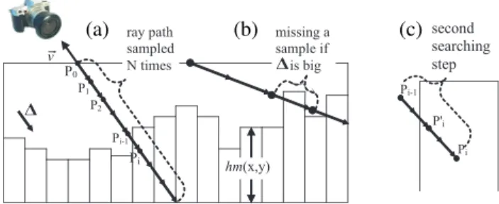
hm(x,y) missing a sample if is big ray path sampled N times P0 P1 P2 Pi Pi-1 v (a) (b) Pi Pi-1 P'i second searching step (c)

Figure 1. Height-map cut view. (a) Searching for the intersection; (b) large ∆ could result in missing information; (c) a second searching step is done to refine the intersection point.

hm(x, y) : [0, 1]2→ [0, 1].

We can define a Boolean function z(P ), for (P.x, P.y, P.z) ∈ [0, 1]3_{, as:}

z(P ) ⇐ ( P.z ≤ hm(P.x, P.y) ) ? true : false, In our implementation, we use the faces of a paral-lelepiped to generate the fragments that will ray cast the height map. The coordinates of its vertices are between 0 and 1 (as in a canonical cube), defining the local coordinate space. The height map data is passed to the GPU through a grayscale texture. The x and y axes of the parallelepiped are exactly coincident with the u and v coordinates of the texture, while z coincides with the height direction.

In GPU, the vertex shader sends to the fragment shader the viewing direction already in local space. This way, each fragment knows the path of the ray inside the canonical cube, and can easily compute its exit point. The fragment shaders main task is to answer the two ray-casting ques-tions: is there an intersection between the ray and the height map? Where is the closest hit point?

As explained in [6], one strategy is to uniformly sample this ray path in N points Pi(see Figure 1(a)) and use func-tion z(P ) to find the ray-surface intersecfunc-tion. This could be implemented by a conditional loop varying Pi, from the entering to the exit point, and stopping when z(Pi) is false. In each step Pi is translated by ∆, which is the ray path divided by N . RayCasting() { P: Point3D P ⇐ ray_origin ∆ ⇐ (exit_point - ray_origin) / N while ( P 6= exit_point and !z(P))

P ⇐ P + ∆ }

(a) (b) (c)

Figure 2. From left to right: the height map, the color map, and the normal map.

When a ray does not intersect any height sample, the fragment should be discarded without any contribution to the frame buffer or to the z-buffer. For fragments not dis-carded, the actual color can be retrieved from a color texture (see Figure 2(b)), and the normal can be either computed di-rectly from the height map or given as a third texture (see Figure 2(c)) to be used for shading. The coordinates used in the texture lookup are (P.x, P.y) right after the iterations. Finally, the depth is computed to register the correct z-value for the z-buffer.

The value of N is a trade off between quality and speed. Some ray-surface intersections may be missed if a large ∆ is used (∆ is inversely proportional to N , see Figure 1(b)).

We propose the following improvements for the height-map GPU visualization:

Two-step searching. Even if ∆ is short enough not to miss a sample, the point where the ray touches the object is not exactly computed. We propose a second searching step be-tween points Pi−1and Pi (see Figure 1(c)). This second step is a binary search that divides the searching domain by two in each step. Therefore, with M steps in the binary search we multiply the precision by a 2M _{factor. Notice} that this second searching procedure is done in the same fragment code, it is not a multi-pass algorithm.

Balancing between steps. Binary search is much more ef-ficient than linear search. However, it cannot be exclusively executed because, along the ray path, there could be several intersections. In other words, the z(P ) function may change different times along the parametric ray for each fragment. On the other hand, when the ray is totally perpendicular to the height map (in a perfect top view), z(P ) will change sign at most once. In this case, the binary search can per-fectly and efficiently compute the intersection without the previous linear search. Based on this observation, we have implemented a balance between the linear and the binary steps according to the viewing slant. When in a vertical view, we reduce the linear search iterations while increas-ing the binary search iterations (N ↓, M ↑). For an almost horizontal viewing direction we do the opposite, prioritiz-ing the linear search (N ↑, M ↓). This way, we achieve up to two times faster rendering for some cases (see Figure 3).

Figure 3. Comparing not-balanced [6] and balanced searches (right column). We obtain better performance when seen from above and better quality when seen in a profile view.

Figure 4. Geometry texture sample. A height map defined inside a hexahedron’s domain.

Non-rectangular height map domain. A height sample with value equal to 0 can be considered either as the surface base or as a representation of empty space. We have chosen the last case, since representing empty space is essential for geometry textures. Figure 6(d) has an example.

3.2

Geometry Textures

The problem approached in our work is different from standard mesostructure rendering. We are interested in re-constructing the details of an entire object, which is a non-repetitive pattern, since it changes over the model domain. In our case, the input is a set of height maps converted from the original model to represent the complete geometrical in-formation.

Geometry textureis a geometric representation for sur-faces. Its domain is a parallel hexahedron and in its interior a height-map represents the surface (see Figure 4). The do-main is not restricted to a perfect rectangle, so empty sam-ples are expected in each geometry texture. The construc-tion of geometry texture patches from a complex model has

no global folding restriction and the patches are well fit-ted around the surface contour. In rendering time, geome-try textures use our ray-casting algorithm implemented in a fragment shader. As a result, the geometry is correctly reconstructed and rendered.

4

Conversion

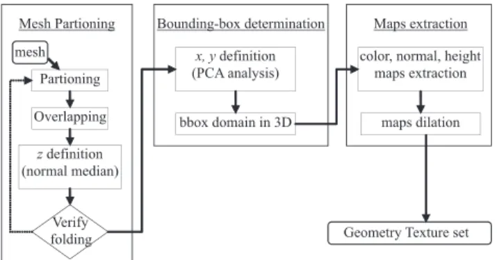
The input for our conversion procedure is a polygon mesh and the output is a set of geometry textures. Fig-ure 5 shows the complete algorithm for converting triangle meshes into geometry textures.

Mesh Partioning Bounding-box determination Maps extraction

Partioning Overlapping Verify folding z definition (normal median) x, y definition (PCA analysis) bbox domain in 3D

color, normal, height maps extraction

maps dilation

Geometry Texture set mesh

Figure 5. Complete procedure for converting polygon meshes into a set of geometry tex-tures. Note that the verify folding step sends a chart back to the partitioning step in case of a overhanging situation.

Among the three conversion steps, mesh partitioning is the most difficult and critical for the success of the algo-rithm. Some conditions are expected when partitioning the input model mesh into charts:

• The chart must not contain a folding situation in its ~z. • The chart domain should be as square as possible to

reduce empty spaces.

• For visualization purposes, neighboring charts must share their boundary, resulting in some overlapping be-tween them. Right after partitioning we add an extra triangle ring around each chart (see Figure 6b). Bounding-box determinationincludes finding a good or-thonormal coordinate system and domain for each one of the charts. Direction ~z is taken as the median normal of all triangles in one chart, with this we minimize the occurence of self-folding partitions. Then, ~x and ~y must be chosen based on the minimization of empty spaces in the domain. We have used the 2D-PCA (Principal Component Analysis)

(a) (b) (c)

(d) · · · (e) · · ·

Figure 6. (a) Mesh partitioning using VSA. (b) Overlapping step, each chart is increased by one ring of triangles. (c) Bounding-box de-termination. (d) Map extraction (height and normal). (e) Map dilation (two-pixel dilation).

algorithm to determine directions ~x and ~y projected on the plane defined by ~z. Finally, we project the coordinates of all triangles to obtain the exact domain in each direction. (~x, ~y, ~z) forms the local coordinate system of the chart.

In the map extraction phase, there are three maps we want to obtain: height, color and normal maps. We have developed a GPU solution to extract the three maps from one chart. Based on the local coordinate system of each chart, we render its triangles in an orthogonal view projec-tion perpendicularly to direcprojec-tion ~z, filling out the viewport with a user-defined resolution (for example, 256 × 256). We repeat the procedure three times capturing the image buffer: • To obtain the color map we render the colors without

illumination.

• To generate the normal map we assign (x, y, z) global coordinates of normal ~niof each vertex vito (r, g, b). During rasterization, within each triangle, the normals are interpolated and then normalized again.

• To obtain the height map we start by finding in CPU the maximum and minimum coordinates (hmax and hmin) in direction ~z. We assign a value hi ∈ [0, 1], computed as hi= _hvi.z−hmin

max−hmin, to each vertex vi. This

value is interpolated inside the triangles and outputted as luminance.

Note that for space-reduction purposes, the image buffer is captured and stored using 8-bit precision.

The rendering algorithm loads the maps as textures. However, before that, we apply a texel-dilation procedure to prevent sampling problems when using mip-mapping. Our

dilation algorithm fills empty texels around the map domain with interpolated values. This procedure is done for normal and color maps. See Figure 6.

In the following subsections we discuss two different strategies we have implemented for mesh partitioning: PGP (Periodical Global Parameterization [8]) and VSA (Varia-tional Shape Approximation [2]).

4.1

Partitioning with PGP

Periodic Global Parameterizationis a globally smooth parameterization method for surfaces. PGP can be applied to meshes with arbitrary topology, which is a restriction in other parameterization methods [8]. Moreover, we can ex-tract a quadrilateral chart layout from this parameterization, which is based on two orthogonal piecewise linear vector fields defined over the input mesh. This orthogonality is es-pecially interesting to guide our partitioning procedure in order to reduce empty spaces in the domain. These vec-tor fields are obtained by computing the principal curvature directions, resulting in a parameterization that follows the natural shape of the surface (left picture on Figure 7).

PGP avoids excessive empty spaces. However, often charts obtained with PGP partitioning present some folding problems. For this reason we have decided to investigate VSA as an alternative partitioning method.

4.2

Partitioning with VSA

Variational Shape Approximation is a clustering algo-rithm for polygonal meshes that can be used for geome-try simplification [2]. Our partitioning algorithm based on VSA uses each cluster as an initial chart, which is further increased to overlap neighboring domains (see Figure 6).

The main advantage of using VSA compared to PGP is that it reduces the number of folding cases. VSA uses L1,2 metric, which is based on the L2 measure of the normal field. This means that it takes into account the normal di-rection of the vertices to cluster them. A folding situation occurs only if vertices in a chart have a sharp difference in their normal direction (over 90 degrees). With VSA, each chart only contains vertices with similar normal directions. In the next section we describe some experiments to compare the PGP and the VSA methods.

4.3

Comparing PGP and VSA

In our tests we have partitioned with both PGP and VSA two different models: bunny and buffle (Figures 6 and 7).

Our first test compares how good PGP and VSA are at avoiding empty spaces. We have counted for each chart the number of used and empty texels. This was done in the four test cases (PGP bunny, VSA bunny, PGP buffle and VSA

buffle). For simplicity, the charts were extracted without overlapping and the maps without dilation. The maximum map size was 128 × 128. A map could be smaller than that (adapted to the chart size), as long as each dimension remained a power of two (respecting OpenGLs restriction). Table 1 shows the results, indicating that PGP is better at avoiding empty spaces.

Model Method Total texels Empty texels % Bunny PGP 1008128 240357 23.84% Bunny VSA 461312 179194 38.84% Buffle PGP 2498048 563652 22.56% Buffle VSA 979456 453069 46.25%

Table 1. Considering empty spaces, PGP is the best partitioning method.

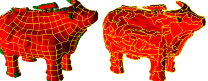
In our second test we have counted how many charts have folding problems, again in the four test scenarios. A way to check if a chart has a folding situation is to verify if there is any inverted triangle when rasterizing all triangles in local direction ~z. Given that the triangles in the mesh re-spect a counterclockwise rotation, if at least one of them is rasterized clockwise then the mesh folds itself in direction ~

z. Figure 7 shows a partitioned buffle model with inverted triangles marked in green. In Table 2 we present the number of folding charts and the total number of inverted triangles found. Clearly, VSA is more appropriate to avoid folding problems.

Figure 7. Buffle partitioning with PGP and with VSA. Triangles with folding problem have their vertices marked in green.

In conclusion, both methods have their own advantages. While PGP is better for reducing empty spaces, VSA is much more efficient in avoiding self-folding charts. We consider that the folding problem is the most important is-sue. Self-folding charts cannot be represented by our ge-ometry texture, which is a strong restriction. On the other hand, empty-space reduction is merely an optimization.

Based on these facts, we have chosen VSA as our par-titioning method (see the total conversion time in Table 3).

Model Method Initial Initial Inverted Folding triangles charts triangles charts

Bunny PGP 69,451 224 817 45

Bunny VSA 69,451 222 3 3

Buffle PGP 117,468 403 2819 62

Buffle VSA 117,468 397 34 6

Table 2. VSA significantly reduces the num-ber of folding charts (identified by inverted triangles).

The results presented in the next section have been achieved using VSA.

Model VSA Bbox Maps Total Memory Bunny 168.9s 6.5s 8.8s 3min 4.2s 1.76MB Buffle 184.4s 20.5s 14.6s 3min 39.5s 3.73MB

Table 3. Conversion times for bunny (222 charts) and buffle (220 charts) using VSA (128 × 128 map size). Most of the effort is in the partitioning step. The last column shows the memory size of generated maps.

5

Results

Once we have obtained a set of geometry textures, we can render them using the GPU height-map ray-casting al-gorithm. In the following sections we discuss performance, rendering quality and memory use.

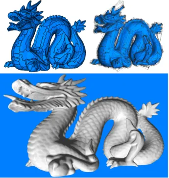
We have used the dragon model with 871,414 triangles for tests (see Figure 8). We have generated three sets of 453 geometry textures, varying their maximum resolution (1282_{, 256}2_{and 512}2_{). The tests were done with a GeForce} 8800 GTX graphics card.

5.1

Performance

Since geometry textures have their performance bottle-necked per pixel, we have varied the zoom level in our tests. We have plotted the results in Figure 9.

To compare performance between geometry textures and common triangle-mesh visualization, we have measured the rendering speed of the original dragon model in two special situations: with Compiled Vertex Array (CVA) and with Ver-tex Buffer Object (VBO). Both methods are advanced fea-tures in OpenGL and without them the speed would be less than 1 FPS for such model size. For the dragon model with 871K triangles, we have obtained 27 FPS with CVA and 135 FPS with VBO (plotted as dashed lines in Figure 9).

Figure 8. Top: Model partitioning and geometry-texture bounding boxes. Bottom:

The dragon rendered with 453 geometry tex-tures with maximum resolution 256 × 256.

0 50 100 150 200 250 300 350 400 0 100000 200000 300000 400000 500000 600000 128x128 256x256 512x512 Mesh VBO Mesh CVA 640x480 800x600 1024x768 1280x1024

Ray-casting area in number of pixels

F

P

S

Figure 9. We have compared three differ-ent geometry texture resolutions (1282_{, 256}2_, 5122) and the original mesh rendered with VBO (Vertex Buffer Object) and CVA (Com-piled Vertex Array) of the dragon model.

The horizontal axis in Figure 9 represents the number of pixels of the dragon’s ray-casting area, which is formed by the rasterization of the geometry-textures bounding-box faces (without recounting overlapping fragments). The higher the number of pixels, the larger the model is on the screen. For a practical idea, we have highlighted some win-dow sizes (640 × 480, 800 × 600, 1024 × 768, 1280 × 1024) which the model would fit.

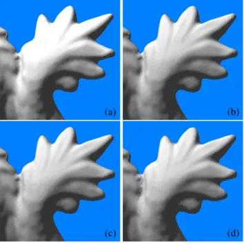
(a) (b)

(c) (d)

Figure 10. (a) Original dragon model with 800K triangles. Dragon rendering with geom-etry textures in different resolutions: (b) 512×

512; (c) 256 × 256; and (d) 128 × 128.

resolution. However, we have verified that the lowest max-imum resolution (1282) was the fastest one. This is a result of less graphics card memory in use (4.21MB), optimizing caching and fetching. As we will see, for quality purposes, 2562_{would be a good choice for maximum resolution for} the dragon’s 453 geometry textures used in test. Its perfor-mance is better than the original mesh rendered with VBO for resolutions smaller than 800 × 600.

5.2

Quality

We have compared image quality by rendering the three sets of geometry textures for the dragon model and its orig-inal mesh. Most visual differences among the four situa-tions appear in the silhouette. For this reason, in Figure 10 we focus on the dragon tail. Geometry textures with 2562_{and 512}2_{are very close to the original mesh rendering.} Based on this observation (which is the same for the whole model), there is no reason in using resolution 5122 _{in this} case, which would multiply by four the memory size com-pared to 2562_{. However, geometry textures with resolution} 1282_{produce an imprecision visible all over the model.} Seamless Rendering

Since we are rendering a model as a composition of patches, an important issue is to assure the continuity of the

recon-(a) (b)

Figure 11. Even if continuous fragments are not rendered by the same geometry texture (a), the final image has no seams (b). There is a z-fighting in the overlapping part, but they are fighting for the same final color.

struction. A perfect junction is possible due to two details in our technique, as has been previously described. The first one is in conversion time: for each patch an extra ring of tri-angles from the neighboring patches (in the dragon exam-ple, we have used four extra rings) is used to generate the geometry textures. The overlap area is necessary to avoid cracks. The second detail refers to the rendering algorithm, and it is based on the fact that the correct z-buffer informa-tion is generated. As shown in Figure 11, continuity is also guaranteed by the correct computation of the final shading over the overlapping parts, based on the normal maps. Per-fragment depth information is also important to maintain compatibility with any other object rendered in the scene.

5.3

Memory

Memory usage is quadratically proportional to the maxi-mum geometry-texture resolution size. In the dragon exam-ple we have obtained: 1282→4.12MB; 2562_{→20.0MB; and} 5122→80.6MB. The dragon’s original mesh uses 13.3MB. We have observed in the discussion about quality that the recommended resolution in our tests was 2562, which has a size compatible to the original model. If memory be-comes an issue, then 1282could be used with the drawback of some precision loss.

6

Conclusion and Future Work

We have proposed a new representation for highly-tessellated models using a set of geometry textures, which are rendered using a GPU implementation of height-map ray casting. Our results have shown that this new represen-tation is suitable for natural models. The final rendered im-ages have similar quality compared to traditional polygonal rasterization methods.

The following items are some of the positive aspects of our technique:

• The rendering speed naturally follows a LOD behavior. This means that when the model is small on the screen (i.e., far from the camera), rendering is faster. This is a result of relieving the vertex-stage burden, transferring computation bottleneck to pixel stage.

• Depending on the chosen resolution, our tion requires less memory than polygonal representa-tion, without losing significant geometry information. • Our technique is compatible with polygon

rasteriza-tion, thus geometry-texture objects can be inserted in any virtual scene composed by polygonal objects. Our potential drawbacks are:

• Recent graphics cards that implement VBO extension have very high performance for polygonal rendering. As a consequence, when compared to VBO perfor-mance, our technique is faster only if the model is not so big on the screen. However, if the scene contains multiple models, polygonal rendering would propor-tionally lose performance, while our solution would keep a stable frame rate.

• Another adverse point is the sophisticated conversion algorithm. Our procedure is composed by multiple passes, including the partitioning step, which is con-siderably elaborate. This may be improved by using multilayer height map (see next section).

We suggest the following ideas for future work:

Image operations on geometry textures. Once we have a new geometry representation based on images (height maps), image operations can be applied on these maps to obtain new results. For example, one could use a low-band filter to smooth the geometry (or a band filter to high-light small geometric features). Image operations to trans-form geometry is a promising application.

Multilayer height-map. The idea is to have only one “ge-ometry texture” to represent the entire model, but with mul-tiple height maps. A unique bounding-box could be used, setting a global height direction (~z). Multiple height-maps can be obtained from the polygonal geometry based on ~

z. In rendering time, a multilayer height-map is rendered also using per-fragment ray casting, considering the layers as forming a CSG (Constructive Solid Geometry) model. Compared to geometry textures, multilayer height-map may have some advantage in reducing implementation complex-ity. In preprocessing, it would skip partitioning and over-lapping steps.

References

[1] L. Baboud and X. Dcoret. Rendering geometry with relief textures. In GI ’06: Proceedings of the 2006 conference on Graphics interface, pages 195–201, Toronto, Ont., Canada, Canada, 2006. Canadian Information Processing Society. [2] D. Cohen-Steiner, P. Alliez, and M. Desbrun. Variational

shape approximation. ACM Transactions on Graphics. Spe-cial issue for SIGGRAPH conference, pages 905–914, 2004. [3] R. L. Cook. Shade trees. In Proceedings of the 11th an-nual conference on Computer graphics and interactive tech-niques, pages 223–231. ACM Press, 1984.

[4] X. Gu, S. J. Gortler, and H. Hoppe. Geometry images.

In SIGGRAPH ’02: Proceedings of the 29th annual con-ference on Computer graphics and interactive techniques, pages 355–361, New York, NY, USA, 2002. ACM Press. [5] M. M. Oliveira, G. Bishop, and D. McAllister. Relief

tex-ture mapping. In Proceedings of ACM SIGGRAPH 2000, Computer Graphics Proceedings, Annual Conference Se-ries, pages 359–368, July 2000.

[6] F. Policarpo, M. M. Oliveira, and J. L. D. Comba. Real-time relief mapping on arbitrary polygonal surfaces. In SI3D ’05: Proceedings of the 2005 symposium on Interactive 3D graphics and games, pages 155–162, New York, NY, USA, 2005. ACM Press.

[7] D. Porquet, J.-M. Dischler, and D. Ghazanfarpour. Real-time high-quality view-dependent texture mapping using

per-pixel visibility. In GRAPHITE ’05: Proceedings of

the 3rd international conference on Computer graphics and interactive techniques in Australasia and South East Asia, pages 213–220, New York, NY, USA, 2005. ACM Press. [8] N. Ray, W. C. Li, B. L´evy, A. Sheffer, and P. Alliez. Periodic

global parameterization. ACM Trans. Graph., 25(4):1460– 1485, 2006.

[9] P. V. Sander, Z. J. Wood, S. J. Gortler, J. Snyder, and H. Hoppe. Multi-chart geometry images. In SGP ’03: Pro-ceedings of the 2003 Eurographics/ACM SIGGRAPH sym-posium on Geometry processing, pages 146–155, Aire-la-Ville, Switzerland, 2003. Eurographics Association. [10] L. Wang, X. Wang, X. Tong, S. Lin, S. Hu, B. Guo, and

H.-Y. Shum. View-dependent displacement mapping. ACM Transactions on Graphics, 22(3):334–339, July 2003.