Acoustic vector-sensor array processing

(1)

Acoustic Vector-Sensor Array Processing

by

Jonathan Paul Kitchens

B.S., Duke University (2004)

S.M., Massachusetts Institute of Technology (2008)

Submitted to the

Department of Electrical Engineering and Computer Science

in partial fulﬁllment of the requirements for the degree of

Doctor of Philosophy in Electrical Engineering and Computer Science

at the

MASSACHUSETTS INSTITUTE OF TECHNOLOGY

June 2010

c

⃝ Massachusetts Institute of Technology 2010. All rights reserved.

Author . . . .

Department of Electrical Engineering and Computer Science

April 26, 2010

Certiﬁed by . . . .

Arthur B. Baggeroer

Ford Professor of Engineering; Secretary of the Navy/

Chief of Naval Operations Chair for Ocean Science

Thesis Supervisor

Accepted by . . . .

Professor Terry P. Orlando

Chairman, Department Committee on Graduate Students

(2)

(3)

Acoustic Vector-Sensor Array Processing

by

Jonathan Paul Kitchens

Submitted to the Department of Electrical Engineering and Computer Science on April 26, 2010, in partial fulﬁllment of the

requirements for the degree of

Doctor of Philosophy in Electrical Engineering and Computer Science

Abstract

Existing theory yields useful performance criteria and processing techniques for acous-tic pressure-sensor arrays. Acousacous-tic vector-sensor arrays, which measure paracous-ticle ve-locity and pressure, oﬀer signiﬁcant potential but require fundamental changes to algorithms and performance assessment.

This thesis develops new analysis and processing techniques for acoustic sensor arrays. First, the thesis establishes performance metrics suitable for vector-sensor processing. Two novel performance bounds deﬁne optimality and explore the limits of vector-sensor capabilities. Second, the thesis designs non-adaptive array weights that perform well when interference is weak. Obtained using convex op-timization, these weights substantially improve conventional processing and remain robust to modeling errors. Third, the thesis develops subspace techniques that enable near-optimal adaptive processing. Subspace processing reduces the problem dimen-sion, improving convergence or shortening training time.

Thesis Supervisor: Arthur B. Baggeroer

Title: Ford Professor of Engineering; Secretary of the Navy/ Chief of Naval Operations Chair for Ocean Science

(4)

(5)

Acknowledgments

Completing a doctoral program is a monumental task for which I have many to thank. I am grateful to God for providing the opportunity, guiding me, and giving me the strength to ﬁnish. He sustained me through three ﬂoods and countless other trials.

My family deserves special thanks. I am deeply indebted to my wife, Amy, for her sacriﬁce during the last four years. Her support and encouragement never wavered; this eﬀort was as much hers as it is mine. She is the love of my life and my best friend. I appreciate the patience of my son, Jack. His laughter and joy made the work easier and always put things in perspective.

Thanks also goes to my parents. They always supported my interest in science, whether they shared it or not. My father taught me to give everything my best. I’m grateful for his wisdom, his friendship, and his example. Before she passed away in 1998, my mother encouraged me to pursue my dream of graduate study at MIT. This thesis is dedicated to her.

The thoughts and prayers of my relatives have lifted my spirits. They are more than a thousand miles away, but I know they are behind me. I am blessed to have them in my life.

I am pleased to thank my advisor, Professor Arthur Baggeroer, for his patience and instruction. He challenged me to make everything better. His time and attention have improved my research, understanding, and writing. I have learned a great deal from his guidance.

I am also thankful for the mentorship of the committee. Meeting with such a distinguished group is a rare privilege. Professor Vincent Chan provided a much needed reality check and encouraged me to think about the context of my research. His advice will help me throughout my career.

Dr. Stephen Kogon deserves extra recognition for the many ways he helped me along the way. First, he helped me learn signal processing at Lincoln Laboratory. Second, he gave me guidance as my Lincoln Scholar’s Program mentor. Third, he sacriﬁced his time to serve on my doctoral committee.

I would also like to thank Dr. Jennifer Watson, my friend and colleague at Lincoln Laboratory. Her faith in me made this experience possible. I cannot thank her enough for standing by me and giving me advice. I will always be grateful for her support.

I appreciate the help of everyone at Lincoln Laboratory who contributed to this work. The sponsorship of the Lincoln Scholar’s Program made this possible and provided an excellent resource. Assistance from the group and division never faltered

(6)

thanks to William Payne and Dr. James Ward. My discussions with Drs. Shawn Kraut and Jordan Rosenthal were invaluable; I thank them again for their time. I appreciate Dr. Nicholas Pulsone for introducing me to “eigenbeams.” I am also thankful for my friend, Kevin Arsenault, with whom it has been a pleasure to work. Ballard Blair deserves recognition for meeting with me almost weekly. I enjoyed our conversations about everything from adaptive processing to z-transforms. Our luncheons will be sorely missed.

Finally, I am pleased to acknowledge Prof. Alan Oppenheim and the DSP Group for their imagination and insight. The one-of-a-kind DSPG brainstorming sessions are some of the most enjoyable experiences of my time at MIT. Special thanks goes to the members: Tom Baran, Sefa Demirtas, Zahi Karam, Joseph McMichael, Shay Maymon, and Dennis Wei. My interaction with them helped form this thesis.

This work was sponsored by the Department of the Air Force under Air Force Contract FA8721-05-C-0002. Opinions, interpretations, recommendations, and conclusions are those of the author and not necessarily endorsed by the United States Government.

(7)

List of Figures

1.2.1 Notional diagram of a vector-sensor . . . 15

1.3.1 Example vector-sensor response patterns . . . 16

1.3.2 Example VSA and PSA response patterns . . . 17

1.4.1 VSA vs. PSA resolution, measured by direction-of-arrival error . . . . 20

1.4.2 VSA beampatterns with “point nulls” and diagonal loading . . . 23

1.4.3 Snapshot deﬁciency: R = 10 km, v = 20 knots, f = 200 Hz . . . . 25

1.7.1 Vector-sensor measurements, scaled to common units . . . 30

2.1.1 A VSA beampattern is easily “mirrored” to any quadrant . . . 39

2.4.1 Notional response of a VSA to point and spread sources . . . 47

2.4.2 Constant gain approximation to uniform spatial spreading . . . 53

2.4.3 Second-order approximation to uniform spatial spreading . . . 57

3.1.1 Example right/left (binary) classiﬁcation scenario . . . 61

3.1.2 Probability of error contours: f = 5 7fd, N = 10 . . . . 67

3.1.3 Probability of error contours: f = 1₇fd, N = 3 . . . . 68

3.1.4 Divergence contours: f = 5₇fd, N = 10 . . . 70

3.1.5 Probability of error contours: f = 5₇fd, N = 10, ∆≈ 0.05 . . . . 71

3.2.1 Example right/left power estimation scenario . . . 72

3.2.2 Left/right power estimation error: f = 5₇fd, N = 10 . . . . 78

3.2.3 Left/right power estimation error: f = 1₇fd, N = 3 . . . . 79

3.2.4 Left/right power estimation error: f = 5₇fd, N = 10, ∆≈ 0.05 . . . . 80

(12)

4.1.2 AMT beampattern: second-order constraints, uniform taper . . . 88

4.1.3 AMT beampattern: second-order constraints, 25 dB Taylor taper . . 89

4.1.4 AMT beampattern: “optimum” null, uniform taper . . . 90

4.1.5 AMT beampattern: “optimum” null, 25 dB Taylor taper . . . 91

4.1.6 AMT beampattern: “oﬀset” null, 25 dB Taylor taper . . . 92

4.2.1 Comparison of tapered point and sector null beampatterns . . . 96

4.3.1 Coarse spatial quantization in cosine-space . . . 99

4.3.2 Example minimax beampattern . . . 103

4.3.3 Eﬀects of mismatch on a minimax beampattern . . . 105

4.3.4 Example minimum sensitivity beampattern . . . 108

4.3.5 Eﬀects of mismatch on a minimum sensitivity beampattern . . . 109

4.3.6 Example endﬁre minimum sensitivity beampattern . . . 110

4.3.7 Eﬀects of mismatch on an endﬁre minimum sensitivity beampattern . 110 4.3.8 Minimum sensitivity versus maximum sidelobe level . . . 112

4.3.9 VSA beampatterns in azimuth and elevation . . . 114

4.4.1 Eﬃciency of an example ﬁxed weighting . . . 116

5.1.1 Adaptive processing in low-dimensional subspaces . . . 119

5.3.1 Integrated error versus eigenbeam dimension . . . 126

5.3.2 Loss incurred with an eigenbeam subspace: D/D0 = 0.4 . . . . 127

5.3.3 Eigenbeam dimension versus frequency and region size . . . 129

5.3.4 ABF comparison with K = 3× D snapshots . . . 130

5.5.1 Eﬃciency of an example subspace processor . . . 132

(13)

Chapter 1 Introduction

Because they are often reliable, easy to analyze, and straightforward to process, pres-sure sensor arrays have dominated sonar for decades. Recent advances in sensor qual-ity and miniaturization have stirred interest in more complex devices, those that mea-sure velocity or acceleration in addition to presmea-sure. Each of these “vector-sensors” provides several measurements, offering significant potential and fresh challenges. Examining the use of vector-sensor arrays in passive sonar reveals the promise such arrays offer to the field of undersea surveillance.1

1.1 Passive Sonar Background

The principles that have historically driven passive sonar research are the same ones behind this work. Therefore, understanding the motivation for this research requires some background in passive sonar. This section provides a brief introduction to passive sonar and pressure-sensor arrays.

Passive sonar, which quietly listens for emitted sound, is eﬀective at undersea surveillance for three reasons. First, sonar operates over great distances. Sound waves sometimes travel thousands of miles underwater. Electromagnetic waves, by contrast, generally travel short distances in saltwater before being absorbed. Second, emitted sound is exploitable. Machinery produces characteristic sounds which aid in

(14)

the detection, localization, and classiﬁcation of vessels. Third, passive sonar is covert. Passive sonar systems are diﬃcult to detect because they emit no energy. Active sonar, by contrast, emits energy which adversaries could use for counter-detection and avoidance.

The most common sensor employed for sonar is the hydrophone. A hydrophone measures only pressure, essentially forming an underwater microphone. Sound waves passing over a hydrophone introduce changes in pressure that are measured and used for detection. Omnidirectional hydrophones are common because their construc-tion, maintenance, and analysis is well-understood. Decades of experience with hy-drophones show they survive well in the corrosive ocean environment and are eﬀective when assembled into arrays.

The most common array configuration is the uniformly spaced linear array. Linear arrays are often fixed to the side of a ship, mounted on the sea floor, or towed behind a moving vessel. When a vessel travels in a straight line, drag pulls a towed array into an approximately linear shape. The exact location and orientation of each sensor is usually unknown or subject to modeling errors.

1.2 Acoustic Vector-Sensors

Increasing the information measured by a sensor generally improves its performance. With acoustic measurements, particle velocity provides additional information about the direction of sound arrival. Acoustic vector-sensors each contain one omnidirec-tional hydrophone measuring pressure and three orthogonal geophones measuring the components of particle velocity.2 _{Figure 1.2.1 illustrates a three-dimensional}

vector-sensor. The geophone in the ﬁgure contains a suspended coil which slides along the axis of a ﬁxed magnet. Sound passing along the axis of the geophone vibrates the coil and induces a current. The induced current provides a measurement of velocity component along the geophone axis.

2_{Although velocity sensors are common, many vector-sensors equivalently use accelerometers,}

(15)

Figure 1.2.1: Notional diagram of a vector-sensor

Although geological vector-sensors have existed for decades, recent advances in geophone design have increased their utility for sonar applications. Because vector-sensors include directional information, they have the potential to improve the per-formance of passive sonar systems.

1.3 Vector-Sensor Processing

Vector-sensor measurements provide more information than pressure-sensor measure-ments. Using this additional information to improve performance is the role of vector-sensor processing. This subsection illustrates the primary beneﬁt of vector-vector-sensor pro-cessing: resolving ambiguous pressure-sensor measurements. Similar, more detailed analyses are provided in [1, 2, 3, 4].

The benefit of vector-sensors is first apparent when comparing a three-dimensional vector-sensor to an omnidirectional pressure-sensor. By definition, the response of the omnidirectional pressure sensor is equal in all directions. But because the vector-sensor also measures particle velocity, a three-dimensional vector, it yields information about the direction of a sound source. Put another way, all directions are ambiguous

(16)

Angle (radians) P owe r (d B ) −π −3π/4 −π/2 −π/4 0 π/4 π/2 3π/4 π -40 -35 -30 -25 -20 -15 -10 -5 0 Dipole Cardioid 3D Limacon

Figure 1.3.1: Example vector-sensor response patterns

of ambiguity means a single vector-sensor is inherently directional. Vector-sensors are also tunable: linear combinations of the four elements forms a “pseudo-sensor” with many diﬀerent response patterns [3]. A few of these patterns are shown in Figure 1.3.1. By choosing appropriate weights, these patterns are easily rotated to emphasize or null any arbitrary direction.

The same behavior extends to arrays of vector-sensors. Compare a uniformly spaced linear array composed of N vector-sensors to one composed of N omnidirec-tional pressure-sensors. Example direcomnidirec-tional responses or “beampatterns” for both array types are shown in Figure 1.3.2. Both arrays have N = 10 elements at frequency

f = 5/7fd, where fdis the design frequency (the frequency at which the inter-element

spacing is one-half wavelength). By choosing weights and linearly combining array elements, the top and bottom plots are “steered” to π/2 and−π/4, respectively. The response of a linear pressure-sensor array (PSA) is symmetric about rotation around the array axis. This is evident in the symmetric PSA beampattern: arrivals from

(17)

op-P owe r (d B ) −π −3π/4 −π/2 −π/4 0 π/4 π/2 3π/4 π -40 -30 -20 -10 0 PSA VSA P owe r (d B ) −π −3π/4 −π/2 −π/4 0 π/4 π/2 3π/4 π -40 -30 -20 -10 0 Angle (radians) PSA VSA

(18)

posite sides of the array yield identical pressure measurements. Changing the weights applied to each element alters the beampattern, but the response is always symmet-ric. The PSA beampattern always exhibits an ambiguous peak, or “backlobe,” in the direction opposite the desired steering angle. In contrast, the vector-sensor array (VSA) utilizes unambiguous measurements from each sensor to reduce the backlobe. The level of backlobe reduction is determined by the choice of weights. In the top plot of Figure 1.3.2, the VSA backlobe is driven near zero; in the bottom plot of Figure 1.3.2, it is reduced by 6 dB.

Directional information makes VSA processing fundamentally diﬀerent from PSA processing. Pressure-sensor processing exploits phase or time-delay measurements to resolve signals and reject noise. Vector-sensors provide little additional phase infor-mation because the sensor components are co-located; the directional components yield mostly gain information. VSA processing must exploit both gain and phase measurements to be eﬀective.

1.4 Problem Statement

The additional measurements provided by vector-sensor arrays oﬀer beneﬁts and chal-lenges. As the previous section shows, vector-sensor arrays are more versatile than arrays of only pressure-sensors. Exploiting this versatility raises a number of ques-tions addressed in this work. These quesques-tions fall into two broad categories that serve to organize the research:

1. How well can a vector-sensor array do? How can the vector-sensor array

“performance improvement” be quantiﬁed? By how much can vector-sensors potentially improve performance?

2. How can a vector-sensor array do well? How can vector-sensor arrays

achieve good performance in practice? Without a priori information, what vector-sensor processing is best? How can vector-sensor processing adapt to incorporate new data? How can the computational cost required to process vector-sensor arrays be reduced?

(19)

Research suggests that existing results do not resolve these questions. Although vector-sensor array processing seems to be a straightforward extension to pressure-sensor array processing, it requires fundamental changes to analyses and algorithms. The remainder of this section highlights the difficulty of answering the above questions with current approaches. Questions in the first category require metrics and bounds to quantify vector-sensor performance. Questions in the second category subdivide according to the two fields of array processing. The first field is nonadaptive processing, where the sensors are combined linearly using fixed weights. The second field is adaptive processing, where weights are allowed to change based upon observed data.

1.4.1 Performance Metrics and Limits

Two performance dimensions commonly used to quantify and bound improvements in array processing are array resolution and gain/directivity. The next two paragraphs brieﬂy show that VSA improvements are not expressed along these performance di-mensions.

Either beamwidth or angle estimation error is typically used to quantify array reso-lution. Figure 1.3.2 reveals that the VSA and PSA beamwidths are almost exactly the same. A wide class of beampatterns, including those in [3, 4], relies on pattern multi-plication (see [5,§2.8]). The width of such beampatterns is virtually unchanged from that of a pressure-sensor array [1, §2.1]. Another metric that quantiﬁes array resolu-tion is the root mean squared error (RMSE) resulting from direcresolu-tion-of-arrival (DOA) estimation. Improving array resolution lowers the RMSE. Bounds on the RMSE are often derived and compared to the actual error of common direction-of-arrival algo-rithms; for vector-sensor arrays this analysis appears in [1, 2, 4, 6]. Representative plots are shown in Figure 1.4.1, derived from [1, §3.2] for the case of a single nar-rowband source in white noise and a N = 13 element, mismatched, linear VSA. The moderate mismatch scenario includes zero-mean Gaussian position, rotation, gain, and phase errors; the direction-of-arrival algorithm is a conventional beamscan tech-nique. A detailed description of the parameters, algorithm, and bound is in [1]. Two

(20)

Array SNR (dB) R M S E (B ea m w id th s) 0 10 20 30 40 50 0 0.1 0.2 0.3 0.4 0.5 0.6

PSA

Beamscan Algorithm

CRB (Lower Bound) Array SNR (dB) R M S E (B ea m w id th s) 0 10 20 30 40 50 0 0.1 0.2 0.3 0.4 0.5 0.6

VSA

Beamscan Algorithm

CRB (Lower Bound)

(21)

observations are clear from the ﬁgure: 1) the actual algorithm RMSE does not de-crease signiﬁcantly with a vector-sensor array, and 2) the lower bound indicates that only a modest improvement is possible. A key consideration is that vector-sensors in-crease the number of measurements from N to 4N , but simply increasing the number of pressure-sensors to 4N (keeping the same inter-element spacing) yields a smaller beamwidth and a lower RMSE. Unlike increasing the number of pressure-sensors, how-ever, using vector-sensors achieves improvement without altering the physical length of an array.

Vector-sensor arrays evidently do not substantially improve resolution, but re-search further reveals that VSAs do not improve directivity more than PSAs with comparable numbers of components. The directivity of vector-sensor arrays, pre-sented in [7], is at most 6 dB higher than pressure-sensor arrays. As with array resolution this improvement is no better than that achieved by simply increasing the number of pressure-sensors from N to 4N .

Because the benefits of vector-sensors are not reflected in measures such as resolu-tion or directivity (considering the increased number of components), new measures are necessary to quantify VSA performance. Although existing bounds are useful for analyzing vector-sensor array configuration [6] and robustness [1], alternative bounds are required to understand how much improvement VSAs offer along the new perfor-mance dimensions.

1.4.2 Nonadaptive VSA Processing

Some of the most powerful nonadaptive processing techniques become diﬃcult or impossible with vector-sensor arrays. Designing ﬁxed weights for nonadaptive pro-cessing involves multiple objectives. Three of the most useful objectives are narrow beamwidth, low sidelobe level, and low sensitivity to modeling errors. Analytical methods enable joint optimization of the PSA beamwidth and sidelobe level, but these methods do not apply to VSAs. As a result, VSA beampatterns are often designed using alternative criteria.

(22)

Many existing approaches are similar to [3, 4] and eﬀectively choose weights to maximize gain against some postulated noise ﬁeld (see Section 4.2). One formulation of this problem is the mathematical program

minimize wH_Rwe

subject to wH_v

0 = 1

(1.4.1)

for some postulated covariance matrix eR and signal replica v0. Choices for the

pos-tulated covariance matrix are often combinations of isotropic noise, white noise, and point sources. The resulting weights may have a simple closed form, and pattern multiplication may allow for spatial tapering. For instance, choosing

e

R = v_bvH_b + σ2I, (1.4.2)

with vb being a signal replica directed at the backlobe, gives “point null”

beampat-terns as shown in the top plot of Figure 1.4.2. Applying a 25 dB Taylor spatial taper ([5, §3.4.3]) to the weights yields the beampatterns shown in the bottom plot.

For a vector-sensor array, optimizing the important objectives of narrow beamwidth, low sidelobe level, and low sensitivity requires new techniques. Because existing tech-niques do not explicitly optimize over these objectives, the resulting weights are sub-optimal with respect to each objective. For instance, the beampatterns in Figure 1.4.2 leave room for improvements in mainlobe width, sidelobe level, and robustness. Techniques that optimize these objectives are widely used for PSA processing, so equivalent techniques for VSA processing are important to develop.

1.4.3 Adaptive VSA Processing

A key problem in adaptive vector-sensor array processing is high dimensionality. Vector-sensor array data is four times the dimension of pressure-sensor array data because of the additional velocity measurements. This high dimension complicates adaptive processing in two ways.

(23)

Untapered P owe r (d B ) −π −3π/4 −π/2 −π/4 0 π/4 π/2 3π/4 π -40 -30 -20 -10 0 Tapered (25 dB Taylor) P owe r (d B ) Angle (radians) −π −3π/4 −π/2 −π/4 0 π/4 π/2 3π/4 π -40 -30 -20 -10 0 σ → 0 σ > 0 σ → 0 σ > 0

(24)

First, it makes parameter estimation more diﬃcult. Adaptive processing often requires estimating the second-order moments of the data, i.e. the covariance matrix. Logic similar to [8] quickly reveals the scope of this problem. The number of indepen-dent observations, or “snapshots,” available is determined by the stationarity of the environment and the length of the array. The environment is eﬀectively stationary if sources move less than a beamwidth during observation. The broadside beamwidths of vector and pressure-sensor arrays are almost the same, ∆θ ≈ 2/N. Recall that N is the number of vector-sensors; the total number of measurements is 4N for a 3-D vector-sensor array. For an array of length L at the design frequency with wavelength

λ, N = 2L/λ. The worst case (shortest) stationarity time is then given by a broadside

source at range R moving tangentially at speed v:

∆Tstat ≈ ∆θ · R/v

= λR/(Lv). (1.4.3)

The time required to preserve accurate phase estimates for a single snapshot is ap-proximately 8× the maximum travel time of sound waves across the array. This travel time is longest at array endﬁre, where it is

∆Tsnap ≈ 8L/c (1.4.4)

for sound wave propagation speed c. The approximate number of snapshots available,

Kavail, is then

Kavail ≈ ∆Tstat/∆Tsnap

= λcR/(8vL2) (1.4.5)

The number of snapshots desired is determined by the dimension of the sample co-variance matrix; a common rule-of-thumb is to use more than two or three times the dimension for a well-estimated matrix [9]. Using fewer snapshots produces weights that are not robust and are sensitive to noise. Assuming an optimistic factor of two

(25)

Array Length (wavelengths)

S n ap sh o ts , K 0 20 40 60 80 100 0 50 100 150 200 250 300 350 400 Desired (PSA) Desired (VSA) Available Length ≈ 18.2λ Length ≈ 11.5λ

Figure 1.4.3: Snapshot deﬁciency: R = 10 km, v = 20 knots, f = 200 Hz

times the data dimension, the number of snapshots desired, Kdes, for a VSA and PSA

are

Kdes,PSA ≈ 2 · N

= 4L/λ (1.4.6)

Kdes,VSA ≈ 2 · 4N

= 16L/λ. (1.4.7)

A typical scenario with R = 10 km, v = 20 knots, and f = 200 Hz yields the curves shown in Figure 1.4.3. These curves illustrate a fundamental adaptive processing problem: the number of available snapshots is usually far fewer than desired. The problem is worse for vector-sensor arrays because of the higher dimension. As indi-cated on the plot, covariance matrices are poorly estimated for vector-sensor arrays longer than about 11.5λ, or N > 23. The same problem exists for pressure-sensor

(26)

ar-rays, but at longer lengths (18.2λ, or N > 36). Adaptive VSA processing techniques must combat this snapshot deﬁciency to be eﬀective in practice.

High dimensional vector-sensor data complicates adaptive processing a second way by increasing the computational requirements. A typical adaptive processing opera-tion, the singular value decomposition of a covariance matrix, generally takes O(N3₎

ﬂoating point operations. A vector-sensor array, then, increases the computational burden by a factor of roughly 43 _{= 64.}

Current approaches for high-dimensional adaptive array processing fall into three categories. The ﬁrst category augments the covariance matrix to make it well-conditioned. Fixed and variable diagonal loading as covered in [10] and [11] take this approach. The second category performs adaptive beamforming in reduced-dimension linear subspaces. Many techniques fall in this category, including some suggested in [4]. The third category utilizes additional information to improve the covariance ma-trix estimate. One such technique is “Physically Constrained Maximum-Likelihood (PCML)” estimation [12]. The problem of high-dimension is more pronounced with vector-sensor arrays, so existing and new techniques must be closely examined.

1.5 Key Findings

This thesis includes several novel contributions to the ﬁeld of array processing. It establishes the limits of VSA performance and describes practical techniques that approach these limits. Organized by chapter, the most signiﬁcant contributions are:

Ch 2: A thorough exploration of vector-sensor array fundamentals. One

key ﬁnding in this area is that many useful properties are not exhibited by vector-sensor arrays. Another key ﬁnding is a real expression for the VSA beampattern.

Ch 3: Two performance bounds on a critical VSA capability: resolving pressure ambiguities. These bounds relate ambiguity resolution to the

(27)

1) the bounds, although fundamentally diﬀerent, both depend on the same sim-ple quantity, and 2) good performance is theoretically possible in most cases.

Ch 4: The design of robust, ﬁxed weights with excellent performance char-acteristics. Key ﬁndings include the “Minimum Sensitivity” criterion, an

al-gorithm for designing robust weights, and a demonstration of improved perfor-mance.

Ch 5: The derivation of optimum subspaces that enable or improve adap-tive processing. Key ﬁndings include 1) the optimality criterion of “inner

product preservation,” 2) the derivation of eigenbeam subspaces as least-squares designs, and 3) a demonstration of signiﬁcant performance improvement.

Several of the contributions listed above are summarized at the end of the thesis in Section 6.1, Figure 6.1.1.

1.6 Sensor and Environment Model

This entire document assumes the same sensor and environment model to simplify discussion.3 _{Each section explicitly notes any departures from or extensions to this}

common model. The subsequent analysis assumes the following sensor model:

1. Co-located sensor components. The hydrophone and three geophones of each vector-sensor are located at the same point and observing the same state. In practice, this requires the component spacing to be small compared with the minimum wavelength.

2. Point sensors. Each vector-sensor is modeled as a single point. In practice, this requires the sensor dimensions to be small compared with the minimum wavelength.

(28)

3. Geophones with cosine response. The signal response of each geophone is pro-portional to the cosine of the angle between the geophone axis and the source. Cosine geophone response results from measuring velocity along only one axis.

4. Orthogonal geophones. The axes of the three geophones are orthogonal. This is true in practice when each vector-sensor is a static unit.

The thesis also assumes the following environment model:

1. Free-space environment. Sound waves travel in a quiescent, homogeneous, isotropic ﬂuid wholespace. This implies direct-path propagation only.

2. Narrowband signals. The signal is analyzed at a single frequency. This means the signal is suﬃciently band-limited to allow narrowband processing in the frequency domain. Passive sonar systems typically operate over a wide, many-octave bandwidth; narrowband signals may be obtained by computing the dis-crete Fourier transform of the measurements and processing each frequency bin.

3. Plane wave propagation. The sound waves are planar at each sensor and across the array. This implies the unit vector from each sensor to the source is the same, regardless of the sensor location. Sound waves are approximately planar when the source is beyond the Fresnel range [8].

The underlying assumptions and notation are similar to those in [2, 6, 13] although this document has a diﬀerent objective.

1.7 Plane Wave Measurement Model

Under the assumptions in Section 1.6, consider a plane wave parameterized by az-imuth ϕ∈ [0, 2π) and elevation ψ ∈ [−π/2, π/2] impinging on an array of N vector sensors. The remainder of the thesis assumes a right-handed coordinate system with

ϕ = 0 as forward endﬁre, ϕ = π/2 as port broadside, ψ = 0 as zero elevation, and ψ = π/2 as upward. The parameters ϕ and ψ are sometimes grouped into the vector Θ for notational convenience. Without loss of generality, assume the geophone axes

(29)

are parallel to the axes of the coordinate system. If this is not the case, the data from each vector sensor can be rotated to match the coordinate axes. The unit vector,

u = [cos ϕ cos ψ, sin ϕ cos ψ, sin ψ]T , (1.7.1)

points from the origin to the source (or, opposite the direction of the wave tion). The following derivations touch only brieﬂy on direct-path acoustic propaga-tion. For a much more detailed study of ocean acoustics, see [14].

Under common conditions, the components of velocity relate linearly to pressure. Assuming an inviscid homogeneous ﬂuid, the Navier-Stokes equations become the Euler equations

∂v ∂t + v

T_{∇v = −}∇p

ρ (1.7.2)

where v is ﬂuid velocity, ρ is density, and p is pressure. For acoustic propagation this equation is linearized, neglecting the convective acceleration term vT_{∇v. With}

a plane wave, the pressure p relates across time t and position x through the sound speed c: p(x, t) = f ( uTx c + t ) (1.7.3) ∴ ∇p = u c · ∂p ∂t. (1.7.4)

Substituting Equation 1.7.4 into the Euler equations in 1.7.2 shows that under weak initial conditions the pressure and ﬂuid velocity obey the plane wave impedance relation

v =−u

ρc p. (1.7.5)

Because the geophones are aligned with the coordinate axes, they simply measure the components of the velocity vector v. The resulting linear relationship between the pressure and each component of the ﬂuid velocity greatly simpliﬁes the analysis of vector-sensor array performance.

(30)

measure-Figure 1.7.1: Vector-sensor measurements, scaled to common units

ments in terms of pressure and the source unit vector. Returning to the array of N vector-sensors, the plane wave measurement of the nth vector-sensor in phasor form is ejk0(rTnu)   1 −u/ρc   (1.7.6)

where rn is the position of the sensor and

k0 ,

2π

λ (1.7.7)

is the wavenumber for a wavelength λ. The term outside the vector is the wave phase delay, which factors out because of Equation 1.7.5. Only the gain diﬀerence between the pressure sensors and geophones is important. For convenience, this thesis chooses a normalization that absorbs that gain diﬀerence into the pressure term:

ejk0(rTnu)  η u   . (1.7.8)

Although this choice of normalization seems arbitrary, it results in simpler expressions later and is similar to the notation used in [2, 6, 13]. 4 _{Also note that this choice of}

normalization requires a factor of (ρc)−2 when comparing beam estimates in units of absolute power.

(31)

The remainder of this thesis uses the gain factor η = 1 in all derivations unless otherwise stated. In most cases, the results are easily extended to arbitrary η, some-times by inspection. The choice of η = 1 for analysis has an important practical motivation involving the trade-oﬀ between left/right resolution and white noise array gain or sensitivity. Although the pressure-sensor often has higher gain (η > 1) for actual vector-sensor arrays, the array data is easily normalized to common units as shown in Figure 1.7.1. Normalizing the units produces two results: 1) a slight loss of array gain because of the increased geophone noise, and 2) an improved ability to resolve ambiguities. Vector-sensor arrays are generally chosen for their ambiguity res-olution, so (2) takes precedent. Put another way, using the η = 1 data normalization strengthens ambiguity resolution at the possible expense of white noise gain.

(32)

(33)

Chapter 2 Elements of Vector-Sensor Array

Processing

Any field, no matter how well organized, possesses a set of fundamentals that must be understood before moving into advanced topics. The field of acoustic vector-sensor array processing is built from elements common to all array processing and elements specific to vector-sensor arrays. The source [5] reviews the former; this chapter introduces some of the latter. Most of the concepts introduced in this chapter are new to the literature and, although simple, have profound consequences.

2.1 Vector-Sensor Array Beampattern

One of the most fundamental differences between vector-sensor arrays and pressure-sensor arrays is the structure of the beampattern. Building on the plane wave mea-surement model provided in Section 1.7, this section provides an expression for the beampattern of an arbitrary vector-sensor array with arbitrary element weighting. It then simplifies this expression for the case of a uniform linear vector-sensor array. The symmetry of the uniform linear array leads to the use of conjugate symmetric weights, a real beampattern, and a reflection symmetry relating beams in one quadrant to the other three quadrants.

(34)

2.1.1 General Complex Beampattern Expression

The most general case for a vector-sensor beampattern is an arbitrary array with an arbitrary, complex element weighting. Beginning with the measurement of a single vector-sensor in Equation 1.7.8, the beampattern of an N -element vector-sensor array is the weighted sum

y(Θ) = N ∑ n=1 w_nHv_n(Θ) (2.1.1) where vn(Θ) , ejk0r T nu(Θ)   1 u(Θ)   (2.1.2)

is the measurement of the nth _{vector-sensor and w}

n are the weights. Recall from

Section 1.7 that rn is the position of the nth vector-sensor, k0 is the wavenumber,

and u(Θ) is the unit vector directed toward Θ. Without knowledge of any sensor positions or constraints on the weights, Equation 2.1.1 cannot be simplified further. It is generally a complex valued expression that is difficult to analyze partly because the unit vector, u, appears both inside and outside the complex exponential. The beampattern at any point is a linear combination of the weights, so defining the array measurement and weight vectors,

v(Θ) , [ vT₁(Θ) vT₂(Θ) · · · vT_N(Θ) ]T (2.1.3)

w , [ wT₁ w₂T · · · wT_N ]T , (2.1.4)

enables writing Equation 2.1.1 as a compact inner product:

y(Θ) = wHv(Θ). (2.1.5)

Sampling the beampattern at a set of M points, {Θ1, Θ2, . . . , ΘM}, corresponds to

the linear transformation

(35)

with

V , [ v(Θ1) v(Θ2) · · · v(ΘM) ] (2.1.7)

y , [ y(Θ1) y(Θ2) · · · y(ΘM) ] T

. (2.1.8)

This linear transformation is valid for any arbitrary vector-sensor array; its real coun-terpart is derived in the next section and forms the foundation of beampattern design via convex optimization in Chapter 4.

2.1.2 Simpliﬁcations Exploiting Symmetry

For a linear vector-sensor array with elements symmetric about the origin, a series of simpliﬁcations to Equation 2.1.1 is possible. These simpliﬁcations allow 1) conjugate symmetry that reduces the number of variables from 8N to 3N and 2) quadrant symmetry that reduces the design burden by a factor of four. This thesis discusses signals in the x-y plane, but the results extend easily to the 3-D case. When dealing with signals in the horizontal plane, the vertical geophone contributes nothing and is ignored. Because the array is linear and the position and direction vectors are in the horizontal plane,

k₀rT_nu(Θ) = d_nk₀cos ϕ (2.1.9) where dnis the position of the element along the array. Ignoring the vertical geophone,

the measurement vector of a single vector-sensor is

vn(ϕ) = ejdnk0cos ϕ      1 cos ϕ sin ϕ     . (2.1.10)

Writing each weight vector in terms of magnitude and phase gives

wn ,

[

anejαn bnejβn cnejγn

]T

(36)

where an, αn, etc. are real. Substituting Equations 2.1.10 and 2.1.11 into Equation 2.1.1 yields y(ϕ) = N ∑ n=1 anej(dnk0cos ϕ−αn) + bncos ϕ ej(dnk0cos ϕ−βn) + cnsin ϕ ej(dnk0cos ϕ−γn). (2.1.12)

Because the element spacing is symmetric about the array center, 1) the vectors v(Θ) are conjugate symmetric and 2) most problems involve only conjugate symmetric weights (see Appendix A.2). The full-length (conjugate symmetric) weight vector, w, is fully characterized by a half-length weight vector,w. Assuming an even number ofe

elements, the parameterization is

L , N 2 (2.1.13) e dl , dL+l (2.1.14) e wl , [ ealejαel eblej eβl eclejeγl ]T (2.1.15) wn =    e w_n_−L n > L e w∗_L_−n+1 n≤ L (2.1.16)

for real variables eal, eαl, etc.. The beampattern in Equation 2.1.12 becomes a real

function when the weights are conjugate symmetric:

y(ϕ) =

L

∑

l=1

2ealcos( edlk0cos ϕ− eαl)

+ 2eblcos( edlk0cos ϕ− eβl) cos ϕ

+ 2eclcos( edlk0cos ϕ− eγl) sin ϕ. (2.1.17)

Note the similarity between the derivation above and the steps involved in FIR ﬁlter design; this aspect of the vector-sensor beampattern is explored more in Section 2.3.

(37)

Using trigonometric identities, Equation 2.1.17 simpliﬁes further:

y(ϕ) = 2

L

∑

l=1

ealcos( edlk0cos ϕ) coseαl+ealsin( edlk0cos ϕ) sineαl

+ eblcos( edlk0cos ϕ) cos eβlcos ϕ + eblsin( edlk0cos ϕ) sin eβlcos ϕ

+eclcos( edlk0cos ϕ) coseγlsin ϕ +eclsin( edlk0cos ϕ) sineγlsin ϕ

= 2 L ∑ l=1 cos( edlk0cos ϕ) [

ealcoseαl+ eblcos eβlcos ϕ +eclcoseγlsin ϕ

] + sin( edlk0cos ϕ)

[

ealsineαl+ eblsin eβlcos ϕ +eclsineγlsin ϕ

] = 2 L ∑ l=1 cos( edlk0cos ϕ) [ eaR l + ebRl cos ϕ +ecRl sin ϕ ] + sin( edlk0cos ϕ) [ eaI l + ebIl cos ϕ +ecIl sin ϕ ] . (2.1.18)

The last step changes from a magnitude/phase parameterization to a real/imaginary parameterization, using the superscriptsRandIindicate the real and imaginary parts of the weights. Four aspects of Equation 2.1.18 are worth noting. First, the conjugate symmetry reduces the number of (real) variables from 6N to 3N . Second, for a linear vector-sensor array with elements spaced uniformly, d units apart, edl = (l−1₂)d. Third,

the mapping from the reduced variables in Equation 2.1.18 to the full, conjugate symmetric weight is a linear transformation. Fourth, the derivation of Equation 2.1.18 assumes even N but is easily modiﬁed for odd N .

The beampattern in Equation 2.1.18 is a simple inner product, the real counterpart to Equation 2.1.5. The single-sensor weight and measurement terms

vl(ϕ) , 2 ·   cos( edlk0cos ϕ) sin( edlk0cos ϕ)   ⊗      1 cos ϕ sin ϕ      (2.1.19) wl , [ eaR l ebRl ecRl eaIl ebIl ecIl ]T (2.1.20)

(38)

yields the full array vectors

v(ϕ) , [ vT₁(ϕ) vT₂(ϕ) · · · vT_L(ϕ) ]T (2.1.21)

w , [ wT₁ w₂T · · · wT_L ]T , (2.1.22)

which are the real counterparts to Equations 2.1.3 and 2.1.4. Writing Equation 2.1.18 as a real inner product gives

y(ϕ) = wTv(ϕ) (2.1.23)

y = VTw, (2.1.24)

the real counterparts to Equation 2.1.5 and 2.1.6, respectively.

Although the beampattern in Equation 2.1.18 cannot be simpliﬁed further without restrictive assumptions, there is another way to exploit the symmetry of the array. The even/odd symmetry of the cosine/sine functions allows any beampattern to be “mirrored” easily to any of the four quadrants. A given beampattern is mirrored across the array axis by changing

ecR

l 7→ −ecRl

ecI

l 7→ −ecIl

. (2.1.25)

This transformation negates the cross-axial component and yields the same response as the original weight on the opposite side of the array. A similar transformation allows cross-axial mirroring, or mirroring from forward to aft:

eaI l 7→ −eaIl ebR l 7→ −ebRl ecI l 7→ −ecIl . (2.1.26)

In this case, the sign changes are a combination of conjugation and negation of the axial component. Performing both axial and cross-axial mirroring, one beam is

(39)

mir-P owe r (d B ) −π −3π/4 −π/2 −π/4 0 π/4 π/2 3π/4 π -40 -35 -30 -25 -20 -15 -10 -5 0 Angle (radians)

Figure 2.1.1: A VSA beampattern is easily “mirrored” to any quadrant

rored to any of the four quadrants. Figure 2.1.1 provides an example beampattern that is mirrored from one quadrant to the other three. The beampattern shown is for a uniform linear vector-sensor array with N = 10, ϕ0 = −π/4, and f = 5/7fd.

In addition to being linear transformations, the mirroring operations only involve sign changes. Mirroring allows eﬃcient conventional beamforming because a single

quadrant of partial sums from each sensor type forms a full set of beams spanning all quadrants with only sign changes. Mirroring also reduces the eﬀort required to design

a set of beams by a factor of four.

2.2 Robustness and the Sensitivity Factor

The sensor and propagation models used in array processing often contain appreciable errors, or “mismatch.” A signiﬁcant source of mismatch is imperfection in the array itself: the exact gains, phases, positions, and orientations of the sensors are unknown. The “sensitivity factor” of a weight vector quantiﬁes its robustness to these modeling

(40)

errors. The (normalized) sensitivity factor of a VSA weight vector, w, is

ξ , vH₀ v₀ wHw

= 2N wHw. (2.2.1)

For weights subject to a unity gain constraint, the Cauchy-Schwarz inequality implies

ξ ≥ 1. The sensitivity factor fully characterizes the deviation of a pressure-sensor

array beampattern under Gaussian errors (see [5, §2.6.3]). The relationship is more complex for vector-sensor arrays ([15]), but ξ remains an eﬀective surrogate measure for the sensitivity of a weight vector to mismatch. Robustness generally decreases as ξ increases, so constraining ξ to be small provides robustness in adaptive beamforming [10]. Section 4.3.3 applies a similar technique to ﬁxed weight design.

2.3 Properties of Linear Vector-Sensor Arrays

Because a pressure-sensor array is a subset of any vector-sensor array, it seems possible that many useful properties of linear pressure-sensor arrays extend to vector-sensor arrays. However, the additional complexity of vector-sensors makes it necessary to re-examine these properties because many require modiﬁcation or do not apply.

2.3.1 Local Fourier Transform Property

One useful property of linear pressure-sensor arrays is that the beampattern is simply the discrete Fourier transform of the weights. This relationship enables using Fourier transform properties and the tools of FIR ﬁltering in design and analysis. The ﬁrst entry in Equation 2.1.10, corresponding to the pressure-sensor, is the complex expo-nential of a Fourier transform vector. For the other components, however, the Fourier transform relationship does not hold because of the sin ϕ and cos ϕ terms outside the exponential.

Although the exact Fourier transform relationship is not valid for vector-sensor arrays, a useful “local” Fourier transform property exists. A small region around any

(41)

nominal point in a linear VSA beampattern behaves like a Fourier transform. The gain of the directional sensors is approximately constant around the nominal angle. Treating the directional sensors as constant introduces some error, ∆v(ϕ), into the array manifold vectors. The error in the resulting beampattern is

|∆y(ϕ)| = wH[∆v(ϕ)]

≤ |w| |∆v(ϕ)|. (2.3.1) The bound in Equation 2.3.1 arises from the Cauchy-Schwarz inequality and is not necessarily tight. If the sensitivity factor is bounded, ξ ≤ α2_{, the magnitude of the}

weight is bounded, |w| ≤ α/√2N . The error in the manifold vector comes only from errors in the directional terms in Equation 2.1.18:

|∆v(ϕ)|2

= 4

L

∑

l=1

cos2( edlk0cos ϕ)(∆ cos ϕ)2+ cos2( edlk0cos ϕ)(∆ sin ϕ)2

+ sin2( edlk0cos ϕ)(∆ cos ϕ)2+ sin2( edlk0cos ϕ)(∆ sin ϕ)2

= 2N · [(∆ cos ϕ)2+ (∆ sin ϕ)2]. (2.3.2)

Substituting the bound on |w| and the expression for |∆v(ϕ)| into Equation 2.3.1 gives |∆y(ϕ)| ≤ √α 2N √ 2N· [(∆ cos ϕ)2_{+ (∆ sin ϕ)}2_] = 2α sin ( ∆ϕ 2 ) (2.3.3) ≤ α · (∆ϕ). (2.3.4)

The last inequality is tight near the nominal angle. Equations 2.3.3 and 2.3.4 are useful for two reasons. First, they prove that in a small region (∆ϕ much less than a beamwidth) around any point, the beampattern approximately equals a weighted

(42)

Fourier transform. Because the pressure-sensor beampattern is a Fourier transform, the vector-sensor beampattern, around a given angle, behaves like a pressure-sensor beampattern. Second, because the deviation of the pressure-sensor beampattern be-tween two sample points is bounded, Equations 2.3.3 and 2.3.4 prove that the devi-ation of the vector-sensor beampattern between two sample points is also bounded. In Chapter 4, this bounded deviation allows a vector-sensor beampattern to be ap-proximated by a ﬁnite set of points with negligible error.

2.3.2 No Modulation or “Steering” Property

The Fourier transform relationship between the weights and the beampattern for a linear pressure-sensor array has many useful implications. One such implication is that modulating the phase of the weights “steers” an arbitrary beampattern (viewed in cosine-space) to any angle. The steered beampattern and the original beampattern have the same shape in cosine-space. In practice, the steering property means that only one real weight – a taper – designed at array broadside is suﬃcient to form identical beams anywhere.

As useful as this property is for linear pressure-sensor arrays, it does not apply to linear vector-sensor arrays. Like the Fourier transform relationship, the modulation property takes a modiﬁed, weakened form with vector-sensor arrays. Separating the vector-sensor measurements into phase and gain components reveals that 1) the phase component exhibits a modulation property in cosine-space like a linear pressure-sensor array, and 2) the gain component is rotated in angle-space by Euler rotations. Although each rotation is a linear transformation of the weight (or equivalently, the data), the gain and phase components cannot be separated by a linear system. Thus, no linear transformation steers a vector-sensor array beampattern to an arbitrary direction. Although the lack of a steering property means each beam must be designed separately, the “mirroring” techniques illustrated in Figure 2.1.1 provide a useful way to reduce the design burden.

(43)

2.3.3 Non-Polynomial Beampattern

Another useful uniform, linear, PSA result associated with the Fourier transform property is that the beampattern is a polynomial function of the variable

z = cos(dk0cos ϕ). This well-known result is easily seen from Equation 2.1.18 by

removing the directional elements, assuming real weights, and applying a Chebyshev polynomial relation to each nested cosine term. The polynomial form of the uniform, linear, PSA beampattern forms the foundation of many tools including Chebyshev, Taylor, and Villeneuve tapers and the Parks-McClellan algorithm [5, §3.4 and 3.6]. Such tools apply polynomial factorizations or approximations to the beampattern in

z-space.

Unfortunately, the vector-sensor array beampattern does not have a similar poly-nomial form. For a polypoly-nomial beampattern representation to be useful, it must be an unconstrained polynomial in some real function z(ϕ). The following discussion sup-presses the dependence of z on azimuth angle, ϕ, when convenient. The single-sensor case illustrates why such a representation does not exist for vector-sensor arrays. Two beampatterns possible with a single vector-sensor are those given by the axial and cross-axial directional sensors:

y0(ϕ) = cos ϕ (2.3.5)

y1(ϕ) = sin ϕ. (2.3.6)

Assume that an unconstrained polynomial representation does exist for some function

z. Because a 2-D vector-sensor beampattern involves three weights, both

beampat-terns must correspond to unconstrained, quadratic polynomials in z, that is,

cos ϕ = a0z2+ b0z + c0 (2.3.7)

sin ϕ = a1z2+ b1z + c1 (2.3.8)

for some real coeﬃcients a0, a1, b0, etc. Breaking the ﬁrst equation into the a0 ̸= 0

(44)

function z to lie in one of the two sets of functions Q0 =    −b0 + s(ϕ) √ b2 0− 4a0(c0− cos ϕ) 2a₀ a₀ ̸= 0, s2(ϕ) = 1, b2 0 − 4a0c0 ≥ |4a0|    (2.3.9) L0 = { cos ϕ− c0 b0 a0 = 0 } . (2.3.10)

The sign function s(ϕ) takes only values of ±1. To reconstruct both beampatterns, any function is further constrained by Equation 2.3.8. The functions in L0 are even

and cannot construct the odd sine function via the composition in Equation 2.3.8. For any function in Q0 to convey sign information about ϕ, the sign function s(ϕ)

must be odd. The form of z is thus restricted to a constant (even) part plus the odd part involving s(ϕ). The even part of the z function must become identically zero when substituted into Equation 2.3.8, leaving the requirement that

sin ϕ∝ s(ϕ)√1 + α cos ϕ (2.3.11) for some real coeﬃcient α. For this to be true and continuous at the origin, α =−1 and

| sin ϕ| ∝√1− cos ϕ. (2.3.12) Because this is clearly not true, no function in Q0 satisﬁes Equations 2.3.8, i.e. no z

function satisﬁes both Equations 2.3.7 and 2.3.8. Thus, no unconstrained polynomial form exists for the single-sensor beampatterns in Equations 2.3.5 and 2.3.6. Further-more, because these beampatterns are possible with any vector-sensor array, VSA beampatterns generally do not have an unconstrained polynomial representation.

Although having a non-polynomial beampattern nulliﬁes the polynomial-based techniques listed above, it does not mean equivalent results are impossible with acous-tic vector-sensor arrays. As Chapter 4 shows, equivalent beampatterns are achievable with techniques not based on polynomial functions.

(45)

2.3.4 Weights With Nonlinear Element-Wise Phase

Weights exhibiting linear element-wise phase are another useful implication of the Fourier transform property of linear pressure-sensor arrays. The modulation property makes real weights designed at array broadside suﬃcient for use at any cosine angle. Real weights, when modulated to another cosine angle, become complex weights with a linear element-wise phase progression.

Because every replica vector on the linear vector-sensor array manifold exhibits a linear element-wise phase progression, it seems that the weights should necessarily exhibit this property as well. To the contrary, Appendix A.2 suggests that vector-sensor weights need not have linear element-wise phase. Chapter 4 proves the exis-tence of such weights by example: many of the custom-designed weights have nonlin-ear element-wise phase progressions. Although weights with nonlinnonlin-ear element-wise phase stray from the concept of “spatial tapering,” they often perform well with vector-sensor arrays. Depending on the design problem, forcing VSA weights to have linear element-wise phase may sacriﬁce signiﬁcant performance.

2.3.5 Nonlinear Physical Constraints

A final property of vector-sensor arrays that deserves clarification is the nonlinearity of the physical constraints. The four measurements of a single vector-sensor are somewhat redundant. The omnidirectional sensor measures the pressure field; the directional sensors measure the gradient of the pressure field.

Although it seems that this redundancy should be easy to exploit, its nonlinear nature leads to complications. Even in the simplest case of the single plane-wave source, the measurements are related quadratically by power. For a single plane-wave source, the sum of the power measured by the directional sensors equals the total power measured by the omnidirectional sensor. With multiple sources, the relationship becomes even more complex and nonlinear. Full exploitation of such physical constraints requires nonlinear techniques such as [12].

(46)

2.4 Spatially Spread Sources with Linear VSAs

It is common scientiﬁc practice to simplify problems by discretizing distributions: point masses in physics, impulses and pure sinusoids in signal processing, and point sources in acoustics. Although these approximations are often extremely accurate, they are sometimes misleading. Modeling spatially distributed sounds as point sources occasionally predicts performance that is unachievable in practice. To avoid such a pitfall, this section derives integrals and approximations for 2-D spatially spread sources as observed by a linear vector-sensor array. The 2-D vector-sensor array is modeled for simplicity, but extending these results to 3-D is discussed where applica-ble. Assuming all spatial processes are zero-mean Gaussian, the quantity of interest is most generally the covariance between two sensors. Because a 2-D vector-sensor measures three quantities, this covariance is size 3× 3 for a single pair and 3N × 3N for an array of N sensors.

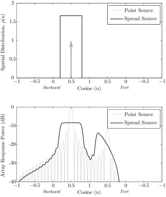
Figure 2.4.1 provides a notional comparison of point and spread sources. The point source corresponds to the impulsive spatial distribution denoted by the gray arrow in the top plot. The response of a vector-sensor array to this point source gives the familiar beampattern shown in the bottom plot. The spatially spread source, by contrast, corresponds to a uniform spatial distribution in cosine-space on the star-board side of the array. The array response to both distributions exhibits sidelobe structure because of the finite aperture and “backlobe” structure because of the pres-sure ambiguity. The spread source integrates power over a range of angles, “filling-in” nulls and widening the array response. The spatial spreading in Figure 2.4.1 is exag-gerated to illustrate its effects on the array response; spatial distributions are often more concentrated than the figure suggests.

2.4.1 General Integral Form

Although spatially spread sources are unexplored with linear vector-sensor arrays, they are common with linear pressure-sensor arrays. Because a pressure-sensor array is a subset of a vector-sensor array, this thesis carefully chooses a spatial

(47)

spread-Cosine (u) S p at ia l D is tr ib u ti o n , ρ (u ) −1 −0.5 0 0.5 1 0.5 0 −0.5 −1 0 0.5 1 1.5 2 Starboard Port Point Source Spread Source −1 −0.5 0 0.5 1 0.5 0 −0.5 −1 -40 -30 -20 -10 0

Starboard _{Cosine (u)} Port

Ar ra y R es p on se P owe r (d B ) Point Source Spread Source

(48)

ing model consistent with the decades of vetted pressure-sensor work. This section extends the model presented in [5, §8.9], analyzing an azimuthal distribution of un-correlated, zero-mean, Gaussian sources. The distribution is speciﬁed in terms of azimuthal cosine (rather than angle), keeping with convention, encouraging closed-form expressions, and restricting the distribution to one side of the array. The results are easily extended to two-sided distributions by expressing any two-sided distribu-tion as the sum of two, one-sided distribudistribu-tions. Because the integrated sources are uncorrelated, the covariance between two sensors is given by the single integral

r01=

∫ +1

−1

ρ(u)v₀(u)v₁∗(u) du (2.4.1)

where u = cos ϕ is the azimuthal cosine, ρ(u) is the spatial distribution of power, and

vi(u) are the responses of each sensor to a signal at u. When the two sensors are part

of a linear vector-sensor array, each response contains a gain term depending only on direction and a phase term depending on both position and direction. If the sensor position along the array axis is x and the gain of each sensor is gi(u), the response is

vi(u, x) , gi(u)ejk0xu. (2.4.2)

The gain terms for the geophone elements are simply the azimuthal sine and cosine expressed in terms of u. Using subscripts o, x, y for the omnidirectional, inline, and cross-axial sensors, these gain terms are

go(u) = 1 (2.4.3)

gx(u) = u (2.4.4)

gy(u) =±

√

1− u2_. _(2.4.5)

The sign of gy(u) changes depending on the side of the array. The remainder of this

(49)

the array. Substituting Equation 2.4.2 into Equation 2.4.1 gives

r(x0, x1) =

∫ +1

−1

ρ(u)g₀(u)g₁∗(u)ejk0x0ue−jk0x1udu

= ∫ +1

−1

ρ(u)g₀(u)g₁∗(u)ejk0(x0−x1)udu (2.4.6)

Equation 2.4.6 is easily written in terms of the distance between the sensors, δ, x0− x1,

and the composite gain function of the sensor pair, G01(u), g0(u)g1∗(u):

r(δ),

∫ +1

−1

ρ(u)G01(u)ejk0δudu. (2.4.7)

Extending the covariance function, r(δ), to 3-D vector-sensor arrays requires no addi-tional work as the elevation terms fall outside the integral. The integral in Equation 2.4.7 is the windowed Fourier transform of ρ(u)G01(u), so a closed form seems

possi-ble. Unfortunately, the number and variety of gain functions make obtaining closed forms for all integrals very diﬃcult with a given spatial distribution. The exact integral form in Equation 2.4.7 does, however, admit several useful and insightful approximations.

2.4.2 Constant Gain Approximation

The simplest and most useful approximation to Equation 2.4.7 arises from the smooth nature of the gain functions and the small width of typical spatial spreading. The standard deviation of the distribution is usually small (less than 5% of cosine-space) when modeling spatially spread sources. Over such a small range of u, the gain func-tions are well-approximated as constant. This constant gain approximation yields a simple but powerful model for vector-sensor spatial spreading using covariance matrix tapers.

When the sensor gains are approximated as constant, incorporating spatial spread-ing simply modulates the existspread-ing covariance function. Without loss of generality,

Acoustic vector-sensor array processing

Acoustic Vector-Sensor Array Processing

by

Jonathan Paul Kitchens

B.S., Duke University (2004)

S.M., Massachusetts Institute of Technology (2008)

Submitted to the

Department of Electrical Engineering and Computer Science

in partial fulﬁllment of the requirements for the degree of

Doctor of Philosophy in Electrical Engineering and Computer Science

at the

MASSACHUSETTS INSTITUTE OF TECHNOLOGY

June 2010

c

⃝ Massachusetts Institute of Technology 2010. All rights reserved.

Author . . . .

Department of Electrical Engineering and Computer Science

April 26, 2010

Certiﬁed by . . . .

Arthur B. Baggeroer

Ford Professor of Engineering; Secretary of the Navy/

Chief of Naval Operations Chair for Ocean Science

Thesis Supervisor

Accepted by . . . .

Professor Terry P. Orlando

Chairman, Department Committee on Graduate Students

Acoustic Vector-Sensor Array Processing

by

Jonathan Paul Kitchens

Abstract

Acknowledgments

Contents

List of Figures

Chapter 1

Introduction

1.1

Passive Sonar Background

1.2

Acoustic Vector-Sensors

1.3

Vector-Sensor Processing

1.4

Problem Statement

1.4.1

Performance Metrics and Limits

PSA

VSA

1.4.2

Nonadaptive VSA Processing

1.4.3

Adaptive VSA Processing

1.5

Key Findings

1.6

Sensor and Environment Model

1.7

Plane Wave Measurement Model

Chapter 2

Elements of Vector-Sensor Array

Processing

2.1

Vector-Sensor Array Beampattern

2.1.1

General Complex Beampattern Expression

2.1.2

Simpliﬁcations Exploiting Symmetry

2.2

Robustness and the Sensitivity Factor

2.3

Properties of Linear Vector-Sensor Arrays

2.3.1

Local Fourier Transform Property

2.3.2

No Modulation or “Steering” Property

2.3.3

Non-Polynomial Beampattern

2.3.4

Weights With Nonlinear Element-Wise Phase

2.3.5

Nonlinear Physical Constraints