Magnetic resonance microscopy of Aplysia neurons : studying neurotransmitter-modulated transport and response to stress

(1)

HAL Id: tel-00979419

https://tel.archives-ouvertes.fr/tel-00979419

Submitted on 16 Apr 2014

HAL is a multi-disciplinary open access archive for the deposit and dissemination of sci-entific research documents, whether they are pub-lished or not. The documents may come from teaching and research institutions in France or abroad, or from public or private research centers.

L’archive ouverte pluridisciplinaire HAL, est destinée au dépôt et à la diffusion de documents scientifiques de niveau recherche, publiés ou non, émanant des établissements d’enseignement et de recherche français ou étrangers, des laboratoires publics ou privés.

studying neurotransmitter-modulated transport and

response to stress

Ileana O. Jelescu

To cite this version:

Ileana O. Jelescu. Magnetic resonance microscopy of Aplysia neurons : studying neurotransmitter-modulated transport and response to stress. Biological Physics [physics.bio-ph]. Université Paris Sud - Paris XI, 2013. English. �NNT : 2013PA112211�. �tel-00979419�

(2)

UNIVERSITE PARIS SUD XI

ECOLE DOCTORALE: Sciences et Technologies de l’Information des Télécommunications et des Systèmes

LABORATOIRE: Unité d’Imagerie RMN et de Spectroscopie, NeuroSpin, CEA DISCIPLINE: Physique

THESE DE DOCTORAT

Soutenue le 2 octobre 2013 par

Ileana O. JELESCU

Magnetic resonance microscopy of Aplysia neurons:

studying neurotransmitter-modulated transport and

response to stress.

Composition du jury:

Directeur de thèse : Denis LE BIHAN Directeur, NeuroSpin, CEA

Encadrante : Luisa CIOBANU Chercheur, NeuroSpin, CEA

Président du jury : Jean-Christophe GINEFRI MCF, Univ. Paris-Sud

Rapporteurs : Paul GLOVER Prof., Univ. of Nottingham

Markus WEIGER Chercheur, ETH Zürich

(3)

(4)

3

This thesis is submitted in partial fulfillment of the requirements for the degree of Doctor of Philosophy by Université Paris Sud.

(5)

(6)

5

y adventure at NeuroSpin started in October 2010, and in the – short – three years that have gone by, I have benefitted from a wonderful working and learning environment, where seniors became mentors and juniors became friends. I would like to express my gratitude to Denis Le Bihan for taking a chance on my unsolicited Ph.D. application and granting me an interview over the phone – a call from Kyoto, where he was working, to Montreal, where I was completing my master degree. I also wish to thank him for his guidance throughout the project, for sharing his extensive knowledge on so many matters and for pushing me to aim ever higher. Very warm thanks to Luisa Ciobanu, for her wonderful daily supervision. I measure how lucky I was to be able to knock on your door whenever necessary (and there has been a lot of knocking…). Thank you for your ever ultrafast feedback/corrections, and for sharing your knowledge and outstanding expertise in physics, microcoils, scanner hardware, troubleshooting, guessing artifacts… I truly appreciated your intellectual honesty, enthusiasm and concern for your students.

I would like to thank Drs. Paul Glover and Markus Weiger for accepting to review this manuscript (over the summer!) and Drs. Jean-Christophe Ginefri and Romuald Nargeot for being part of the jury.

I am also grateful to Romuald for teaching me everything I know about Aplysia and for bringing an indispensable biological expertise to our studies on living tissue. Thank you for your kindness and patience, and for encouraging me to trust my physicist hands and perform meticulous biological tasks. I have fond memories of our trips to Arcachon, picking up Aplysia at low tide.

Françoise Geffroy is the person who took over when my dissection skills reached their limits: thank you for your help with isolating single cells and for your enthusiasm to image them under your microscope and watch them “talk to their neighbors”! Thank you also for your indefectible good mood, sounding laughter, kindness to everyone and excellent “macarons”!

Another remarkable collaboration I would like to mention is that with Nicolas Boulant, who knows the physics of selective excitation inside out and wrote the code to design the DESIRE pulses. Thank you for encouraging me whenever I was

M

(10)

9

depressed with my experiments (the physics cannot be questioned, so “it should work”) and for providing me with precious advice on numerous matters.

I would like to thank Pierre Marquet for spending several months at NeuroSpin to perform DHM experiments in parallel with my diffusion MRI ones. I learned a lot about your technique and very much appreciated all of our conversations. Switzerland sounds like a wonderful place!

My gratitude also goes to the electronics team – Eric Giacomini and Marie-France Hang – for getting me started on coil design and building, as well as to Jérémy Bernard for fabricating numerous stands and supports for my – otherwise shaky – experimental set-ups. Many thanks also to Boucif for his help with Aplysia tending (it’s a lot of work!), and to Denis F, Maryline, Emmanuelle, Elisabeth and Nathalie for their help with purchasing substances and gizmos, and other organizational matters.

Thank you to all the temporary residents of the open space 1025A who made every day enjoyable and with whom I have shared so many joyful coffee breaks, lab beers and conference outings: Benjamin, Julien F, Céline, Nadya, Alfredo, Guillaume, Rémi and Marianne. The first four are now safe, happy and sound; good luck to the remaining four in the completion of your PhDs! I hope the museum of horrors will keep expanding. I would also like to thank Ioana and Dominique, who kept our open space clean and could tell from a distance whether I was having a good or a bad day. I would like to mention all the people with whom I have had highly entertaining scientific and less-scientific conversations at lunch breaks, lab and scientific meetings, or on the train to Paris: Benoît L, Sébastien, Fawzi, Julien V, Franck, Aurélie, Alexandre, Cyril, Fabrice, Alexis, Tom, Mami, Shun, Chris, Karl, Jing, Béchir, Aurélien, Martijn, Alice, Clarisse, Delphine, Véronique, Benoît S and Chloé. Very special thanks go to Olivier, for getting me started with the scanner and programming in ParaVision, then gradually putting up with me every day and eventually becoming the best life sidekick – I look forward to our forthcoming adventures!

I am finally very grateful to my family and friends, for letting me be who I am and do what I love, and accepting that I have chosen to spend three years studying a sea slug instead of getting “a proper job”.

I dedicate this thesis to my father, an engineer, who would have been very happy to know I am still doing science.

(11)

10

ecent advances in the life sciences have had a tremendous impact on our understanding of physiology and pathology, and eventually on our life comfort. However, faithful to the popular wisdom that the more you know, the less you understand, new findings raise ever more questions. This is particularly applicable to the study of living systems, which appear under many aspects to be anything but deterministic. One natural way of trying to explain the unexplained is to take a closer look – a microscopic look. This is roughly the philosophy behind this thesis. While the advent of magnetic resonance imaging (MRI) in the clinic has irreversibly transformed many fields such as radiology, medical research and neurosciences, there are observations which currently have no definite explanation. For instance, cerebral ischemia has been known to cause a decrease in water diffusion in the brain, likely related to the membrane depolarization and cell swelling caused by ischemia. The exact mechanism has however not been established, yet diffusion MRI is used routinely in the clinic for the diagnosis of acute ischemia. Similarly, the manganese ion (Mn2+_{), used as an MR contrast agent in animal studies, is known to} be transported along neural pathways, up to distant regions with brain activation. However, the exact mechanisms of its transport, whether synaptic or non-specific, have not been fully elucidated.

One drawback of MRI is its poor sensitivity, which is translated into relatively low spatial resolution images. Yet one feels that truly useful insight could be brought into the questions raised above if one could image what happens in the brain at a cellular scale. This is where magnetic resonance microscopy comes in. This technique consists in acquiring MR images of small samples at much higher resolution than usually typical for MRI, e.g. 20 µm versus 1 mm. Yet 20 µm is perhaps still too coarse for the human brain, with its 4 µm neuronal bodies and hundreds of trillions of synapses. So let us then take a microscopic look at a nervous system with larger structures: that of Aplysia californica, with its neuronal bodies several hundred microns in diameter and some 20,000 neurons in total.

The global objective of this thesis was therefore to use magnetic resonance microscopy techniques for the study of fundamental aspects of the nervous system at the level of individual neurons and their networks. The strength of combining MR microscopy with the Aplysia model is the potential to exploit all the richness of MR

(12)

11

contrast mechanisms for the study of an almost fully determined neuronal network. Two approaches were chosen, corresponding to the two questions raised earlier. On the one hand, the study of Mn2+_{transport inside a neuronal network, tracked with} manganese enhanced MRI, and its ability to accurately trace axonal projections and neurotransmitter-modulated communication. On the other hand, the diffusion changes induced by membrane depolarization and cell swelling, tracked with diffusion-weighted MRI at two structural scales: at the level of overall nervous tissue and inside the neuronal body.

For these biological experiments to be possible, important MR hardware and methodology needed to be developed. These include the design, building and testing of dedicated transceiver coils, and the development and implementation of appropriate sequences, in particular for diffusion measurements. (This is not to mention the setup from scratch of an aquaria section in the animal house of NeuroSpin and daily tending for the Aplysia.)

This thesis is organized into three parts. The first part serves as an introduction to the basic principles of MRI (Chapter 1) and to the main challenges and achievements of magnetic resonance microscopy (Chapter 2). It also deals with what the author has called “materials”: a description of both the animal model and the hardware used for the experiments, in particular the design and performance of the micro-coils (Chapter 3). The second part provides an introduction to MR contrast agents and to manganese enhanced MRI (Chapter 4) and covers the study performed on neurotransmitter modulated Mn2+_{transport in the Aplysia} (Chapter 5). The third part is dedicated to diffusion MRI. Chapter 6 reviews the principles of diffusion weighted MRI, its main applications and challenges. Chapters 7 and 8 deal with the implementation and phantom validation of two diffusion sequences particularly suited for microscopy: 2D DESIRE (Diffusion Enhancement of SIgnal and REsolution) and 3D DP-FISP (Diffusion-Prepared Fast Imaging with Steady-state free Precession). Chapter 9 makes extensive use of the DP-FISP sequence to carry out the study on tissue and cellular diffusion changes in response to stress.

(13)

12

Part I

MR microscopy: General

concepts and methodology

(14)

13

hen medical and biological applications of MRI started developing in the 1970s, the aim was to achieve whole body imaging in humans. Within hospitals and research centers, this new modality quickly became very popular, as it was non-invasive and allowed the visualization of tissues with an unprecedented variety of contrasts.

The idea behind magnetic resonance microscopy (MRM) is to apply the potentiality of MRI – tissue preservation and diversity of contrasts – to small, living, biological samples. The first achievement of this was the publication of an MR image of an ovum from Xenopus laevis (Aguayo et al., 1986). This first MR image of a single cell allowed the visualization of the nucleus and of the vegetal and animal poles within the cytoplasm. The spatial resolution of the image was 10x13 µm in-plane with a 250 µm thick slice. MRM has since developed into a full-fledged field, with its very own requirements, limitations and specificities.

The scale boundary between MRI and MRM is not clear-cut. It is generally accepted that images with spatial resolution below 100 µm pertain to microscopy. However, it would perhaps be more appropriate to refer to such a “boundary” in terms of voxel volume, because reported high in-plane spatial resolutions (< 10 µm) usually come with thicker slices. Let us then say that MRM images are generally associated with voxel volumes on the order of the nanoliter, which corresponds to a 100 µm cubic voxel.

Compared to optical imaging or even more so to atomic force microscopy, the spatial resolution achievable with MRM might seem unworthy of the term “microscopy”. However, MRM should always be regarded as complementing other microscopy techniques. Its major advantages are the non-invasiveness and the variety of information it can provide, while its major drawback is the poor inherent sensitivity.

(15)

14

1. MRI

he development of magnetic resonance imaging (MRI) was a two-step process: the first step was the discovery of the nuclear magnetic resonance (NMR) phenomenon and its application to the spectroscopy of liquids and solids, separately by Bloch and Purcell in 1946. The second step was taken in 1973 by Lauterbur and later Mansfield, who developed the idea of using magnetic field gradients to spatially encode the NMR signal and produce an NMR image (Lauterbur, 1973). This chapter will very briefly present the concepts behind MRI, in particular those needed to understand the challenges of MRM. For a more detailed description of MRI, one can refer to specialized literature (Haacke et al., 1999; Nishimura, 1996).

1.1 NMR

NMR is a quantum phenomenon that can be observed in nuclei with an odd number of protons and/or neutrons. These nuclei possess a non-zero spin angular momentum

S, usually simply referred to as “spin”. In biological tissue, the most common

elements with a non-zero nuclear spin are hydrogen (1_{H), sodium (}23_{Na) and} phosphorus (31_{P). Hydrogen nuclei} (or simply “protons”) are by far the most abundant, given the large proportion of water in tissue. All of the experiments performed in this work pertain to proton imaging.

A charged particle with a non-zero spin also possesses a small magnetic moment μ:

⃗ ⃗ (1.1)

where is the gyromagnetic ratio and is nuclei dependent. For protons, ⁄ ⁄ .

In the presence of an external magnetic field B0 = B0z, the magnetic moment μ is endowed with a potential energy equal to:

⃗ ⃗⃗ (1.2)

(16)

1. MRI

15

where ħ is Planck’s reduced constant and ms are the magnetic quantum numbers which take on discrete values: in the case of the proton. This results in a splitting of the nuclear energy levels known as the Zeeman effect. In other words, for protons, two energy states are available: a lower one (also referred to as “parallel’ or “spin-up” state) corresponding to ⁄ and a higher one (also referred to as “anti-parallel” or “spin-down” state) corresponding to ⁄ .

Because the “parallel” state corresponds to a lower energy state, its population n+ slightly exceeds that in the “anti-parallel” state (n-), in a ratio given by the Boltzmann distribution:

( _{) (} ₎ (1.3)

where k is Boltzmann’s constant and T is the absolute temperature. In practice, at room temperature, nuclear magnetic energies are much smaller than thermal energies and therefore the excess of the parallel population is very small, typically 1 to 10 out of 106_{. Nonetheless, it is sufficient to produce a net macroscopic} magnetization M in a sample, which is aligned along B0 at equilibrium. The

intensity of the equilibrium magnetization M0 in the Curie regime (i.e. ) is

proportional to the applied static field and to the proton density 0 in the sample, and inversely proportional to the temperature:

(1.4)

Transitions between the two quantum states occur when the spins are excited by an electromagnetic wave with photon energy ħ equal to the energy gap between the parallel/anti-parallel states . The corresponding frequency of the electromagnetic wave, called resonant (or Larmor) frequency, is therefore equal to B0. With current magnetic field strengths comprised between 1.5 T and 21 T, Larmor frequencies fall within the radiofrequency (RF) range (64 –900 MHz).

NMR is by nature a quantum phenomenon and all its theory can be derived from quantum mechanics. However, a classical mechanics description of a magnetic moment in a magnetic field is often adopted for simplicity. This classical standpoint is justified by the fact the expectation values for the proton magnetic moment derived from quantum mechanics are eventually governed by classical equations. For convenience, a classical description of NMR will also be adopted in this thesis.

(17)

16

From a classical standpoint, the application of a resonant electromagnetic field B1,

perpendicular to B0, results in the tipping of the macroscopic magnetization M away

from its equilibrium orientation (i.e. away from the axis of B0, traditionally labeled z). The flip angle α, by which the magnetization is tipped away from z, is dependent

on B1 amplitude and duration through:

∫ (1.5)

When B1 is switched off, the out-of-equilibrium magnetization M will keep

precessing around the z-axis at the Larmor frequency. A receiver coil oriented transversally to z will pick up changes of magnetic flux generated by the rotating magnetization in the form of induced current. This current is the NMR received signal, which comes solely from the transverse component of M.

Once the system is out-of-equilibrium and not supplied with energy (B1 is off), it will

also relax back to its equilibrium orientation (along B0) while precessing. In NMR,

there are two separate relaxation processes, one for each of the two projections of M: the “longitudinal” component along the z-axis, and the “transverse” component in the xy-plane.

The first process is referred to as spin-lattice, longitudinal or T1 relaxation. It consists in the gradual increase of the longitudinal component Mz of M up to its equilibrium value M0, a growth empirically described by an exponential recovery with a time constant T1. This process stems from the interaction between a spin with its surrounding atomic and nuclear lattice. The energy involved in the transition between two proton spin states is compensated by an opposite transition (requiring the same amount of energy) between lattice states. Because it is related to energy exchanges between the spins and the lattice, T1 depends on the chemical and physical properties of the spins’ environment. T1 also increases with B0.

The second process is referred to as spin-spin, transverse or T2 relaxation. It consists in the gradual decrease of the transverse component Mxy of M, empirically described by an exponential decay with a time constant T2. This relaxation is caused both by spin-lattice and spin-spin interactions, and therefore T2 ≤ T1. Spin-spin interactions refer to a collective dephasing effect. The local field experienced by a spin is indeed modified by the fields of its neighbors, resulting in a modified local precessional frequency and global dephasing between spins in time. In biological tissue, spin-spin interactions typically dominate the transverse relaxation process and therefore

(18)

1. MRI

17

T2 << T1. T2 also depends on the chemical and physical properties of the spins’ environment, but is less dependent on B0.

The behavior of the nuclear magnetization M is therefore described by the following phenomenological relationship, known as the Bloch equation:

⃗⃗⃗

⃗⃗⃗ ⃗⃗

⃗ ⃗ ⃗ _(1.6)

In this equation, B is the sum of the various magnetic fields (B0, B1…) applied at a

given time t, and x, y, z are the unit vectors in the x, y, z directions, respectively. The cross-product term describes a precessional behavior at a frequency B, while the second and third terms describe the exponential relaxation of the transverse and longitudinal components, respectively.

Using a complex formalism, the solution for the transverse component of M in the presence of B0 only is:

(1.7)

Assuming a receiver coil that is uniformly sensitive over the sample, the NMR signal s(t) picked up will be proportional to the volume integral of Mxy(t).

Considering a homogeneous sample (e.g. a water phantom), the signal recorded from a simple NMR experiment – excitation / reception – oscillates at a frequency 0 within an envelope that decays with time constant T2. This signal is called free-induction decay (FID). If the magnetic field throughout the sample is not perfectly homogeneous, the magnetizations at different spatial locations will precess at different frequencies, leading to a global loss of coherence when adding up, and to a more rapid decay of the overall measured signal. This new time constant is referred to as T2*, with T2* ≤ T2.

In practice, the static magnetic field throughout a sample is never perfectly homogeneous. Although the homogeneity of an unloaded magnet is a crucial specification of MR systems, placing a sample and a coil inside the magnet will necessarily produce additional distortions in the field. This effect is enhanced at ultra-high fields and at interfaces (e.g. air/water), because of magnetic susceptibility mismatches. In an attempt to minimize static field inhomogeneities specific to each experimental setup (i.e. sample and probe dependent), magnets come with sets of “shim” coils. To improve homogeneity in a given volume of interest, the current in

(19)

18

each shim coil is adjusted to counteract part of the B0 variations in that volume. The complexity of the shimming process is well described in (Chmurny and Hoult, 1990). Briefly, the behavior of the static field inside a magnet through which no current flows is governed by the Laplace equation:

(1.8)

In traditional polar spherical coordinates (r, θ, ), the solution to Equation (1.8) can be expressed as an expansion in spherical harmonics:

∑ ∑ [ ]

(1.9)

where a is the average magnet radius, Cnm and nm are constants, and Pnm are associated Legendre polynomials. The only harmonic that represents a homogeneous field is the one for n = 0 and m = 0. All the other harmonics are error terms that must be set to zero. Although there is an infinity of them, in practice only harmonics of order n up to 5 (and in fact most often 2) are considered, because beyond that the factor (r/a)n_{becomes negligible for a small volume (r << a). The idea behind} shimming is to introduce additional fields that cancel all unwanted harmonics (Golay, 1958).

Ideally, each shim coil should generate a single harmonic, the amplitude of which is meant to cancel the one in the main static field. In practice, the current in each shim coil also generates lower and higher order harmonics, hence the complexity of the problem. The current in each shim coil can be manually adjusted by the operator at the magnet console but most frequently automatic algorithms are provided for shimming at various levels: in the global sensitive volume of the coil (usually first order shims, n = 1), or within a particular region of interest (usually involving second order shim, n ≤ 2) (Gruetter, 1993; Kanayama et al., 1996). The main pitfall of shimming is finding a local, rather than the global optimum solution. Good practice for successful shimming begins with centering the probe with respect to the origin of the shim coils.

(20)

1. MRI

19

1.2 Magnetic field gradients and imaging

In the case of a non-uniform sample, such as biological tissue, it is interesting to differentiate the contributions of protons at different locations in the sample to the overall signal, as they may have different properties (e.g. proton density, T1, T2…). The idea behind this achievement was hinted at in the previous section: if experiencing different magnetic field strengths, local magnetizations will precess at different frequencies.

Following excitation (i.e. B1 is off) and ignoring inhomogeneities, if a magnetic field

gradient G(t) is added to the main field B0, the Bloch equation becomes:

⃗⃗⃗ ⃗

⃗⃗⃗ ⃗ ⃗ ⃗ ⃗

⃗ ⃗ ⃗ ⃗ ⃗ ⃗ _(1.10) Using the complex formalism, the solution for the transverse component of the magnetization, starting from any initial condition m(r), is therefore:

⃗ ⃗ ⃗ ∫ ⃗ ⃗ (1.11) In the interest of clarity, we will ignore T2 relaxation for now and consider the signal demodulated by 0. The received NMR signal is:

∫ ⃗ ∫ ⃗ ⃗ ⃗ (1.12)

We define a space of spatial frequencies, or k-space, in which the location is given by the time integral of the gradient waveforms. If i refers to either dimension x, y or z, the k-space location at a given moment during the acquisition is given by:

_∫ (1.13)

Hence Equation (1.12) becomes:

(21)

20

In this form, it appears that the NMR signal measured at a given time t is the 3D Fourier transform (FT) of the sought magnetization map m(r), evaluated at spatial frequency coordinates k(t). Once this FT is evaluated over a sufficient range of k-space, the inverse FT can provide a reasonable estimate of m(r).

In Cartesian sampling, there are two dedicated paths for acquiring information from a given coordinate in k-space. One way is to apply a constant gradient while the signal is being acquired, thus “moving” along one direction in k-space. This gradient is referred to as “frequency encoding” or “read-out” (ro) gradient and its direction is traditionally labeled “x”. The successive signals recorded by the analog-to-digital (A/D) converter in the reception pipeline will thus map one line in k-space along kx. The second way is to apply a gradient in-between the excitation and the reception blocks. This gradient is referred to as “phase-encoding” (pe) gradient and its direction is traditionally labeled “y” for the second dimension and “z” for the third. The phase-encoding gradients bring the system at a given coordinate along ky (and kz) prior to read-out, but this coordinate remains constant during signal reception. In two dimensions, if the sought image is an NxN matrix, then the typical MR imaging scheme will be the repetition of excitation/encoding/acquisition with N phase-encoding steps, and the acquisition of N samples during each signal read-out. The extension to 3D acquisitions (mainly used in this work) is straightforward by introducing a third gradient Gz and taking the 3D inverse FT of the cuboid k-space thus filled.

In order to retrieve m(r) through inverse FT, the k-space should be covered and sampled “sufficiently”. Let us specify what this means. Relationships between position r and spatial phase k will allow us to define crucial imaging parameters. The spatial resolution of the MR image along dimension i ( i) is determined by the maximum position attained in k-space along i, which in turn is governed by the maximum gradient areas attained by the read-out or phase-encoding gradients:

(1.15)

The field-of-view (FOV) covered by the image is determined by the spacing between samples in k-space along i:

(22)

1. MRI

21

For the read-out direction, this is dictated by the product of Gx and the dwell time of the A/D converter. For the phase-encoding directions, this is dictated by the product of the incremental gradient amplitude step and phase-encoding duration.

For simplicity, we have described the protocol for a line-by-line Cartesian filling of k-space, illustrated in Figure 1. If the successive lines are acquired starting from one edge of k-space (e.g. -ky,max) and gradually moving towards the furthest opposite position (ky,max) then the encoding is referred to as linear. If the first line acquired is the central k-space line (ky = 0) and the successive encoding steps allow the acquisition of lines for increasing |ky|, then the encoding is referred to as centric. An extremely popular accelerated version of the Cartesian scheme is the echo-planar imaging (EPI), which consists in acquiring all (single-shot) or a subset of (multi-shot) the lines in k-space following a single excitation (Stehling et al., 1991). Now that the relationship between k-space and image space is clear, it is also important to mention that different k-space sampling strategies, such as radial or spiral (Ahn et al., 1986), are also possible by simultaneously applying appropriate gradient waveforms on two or three axes. However, such data need to be re-gridded before applying the FT to obtain the image.

Figure 1. A: Cartesian sampling of 2D k-space. The furthest position reached and the spacing between points determine the image resolution and FOV, respectively (see Equations (1.15) and (1.16)). The gradients played to produce the trajectory outlined in red are represented in B. The relative gradient intensities and durations are to scale. The

phase-encoding time is also used to reach –kx,max in the read-out direction by applying a

dephasing lobe of half-area and opposite polarity. During “read-out”, the analog-to-digital converter is on and the signal is sampled at an appropriate rate to fill the matching points in k-space. Tx: transmission / Rx: reception.

(23)

22

1.3 Echoes, timings and sequences

As mentioned earlier, the FID following excitation will decay with a time constant T2* due to magnetic field inhomogeneities. Let us concentrate on the acquisition of the central k-space line. The introduction of the dephasing read-out gradient lobe (see Figure 1) translates into additional dephasing and even more rapid signal decay. However, the position-dependent phase thus accumulated by the spins is undone when the read-out gradient is switched on, with an opposite polarity to that of the dephasing lobe. When the gradient areas are compensated (i.e. the center of k-space is reached), the signal is restored to the level of the T2* decay envelope: this signal resurrection is referred to as a gradient echo.

The effect of constant field inhomogeneities can also be undone and the amplitude of the echo restored to the level of the T2 decay envelope. This signal resurrection is then referred to as a spin echo, and is typically achieved by introducing a refocusing RF pulse before the read-out. Spin-echo sequences are based on 90° excitations pulses and 180° refocusing pulses. Figure 2 illustrates the effect of a 180° refocusing pulse on the dephased magnetization: the “faster” spins are given a negative phase advance and the “slower” spins a positive one, so that at echo time they are all in phase again.

Spin-echo sequences are typically slower than gradient echo ones and deposit more RF energy. However, they are by design insensitive to magnetic susceptibility artifacts and produce higher signal levels. Figure 3 shows basic timing diagrams for

Figure 2. Schematic of the effect of a refocusing pulse. Following a 90° excitation, the spins gradually dephase due to local magnetic field inhomogeneities. The “blue” spin has a phase advance and the “red” spin a phase delay. By applying a 180° flip angle at TE/2, the magnetization configuration is flipped such that the “faster” blue spin has a phase delay and the “slower” red one has a phase advance. At TE they will thus all come into phase again and the overall signal will be at its strongest. TE: echo time. The pulse subscript gives the axis around which the magnetization is flipped.

(24)

1. MRI

23

gradient echo and spin echo. Echo time (TE) and repetition time (TR) are crucial sequence parameters that influence signal-to-noise ratio (SNR), acquisition time (TA) and most importantly image contrast.

Indeed, the richness of MRI comes from the fact that the signal level in the image is a function of many parameters, intrinsic and extrinsic. The extrinsic parameters are related to sequence design, such as excitation flip angle α, TR or TE. The intrinsic parameters are for example free water proton density (PD) or relaxation times T1, T2 and T2*. The extrinsic parameters can be chosen so that the signal is more or less weighted by each of the intrinsic parameters. For example, a long TE produces T2 weighting in spin-echo sequences and T2* weighting in gradient echo sequences. T1 weighted images can be obtained from gradient echo sequences with short TR and TE. This feature of MRI is important because proton density for instance varies little across biological tissue, but T1 and T2 weighted images allow to differentiate between structures at many different levels (between gray and white matter in the brain, between healthy or cancerous tissue, between cytoplasm and nucleus within a cell…).

From the basic gradient echo and spin echo sequence blocks described above, a certain number of important sequence-types emerged. We will briefly describe the concepts behind the ones that have turned out to be of interest in this thesis work. Figure 3. Timeline of events for basic gradient echo (A) and spin echo (B) acquisitions. A 3D Cartesian acquisition scheme is represented, with phase-encoding gradients on two axes. The A/D converter (not shown) is on concomitantly with the read-out gradient.

(25)

24

FLASH (Fast Low Angle SHot) and TurboFLASH

The FLASH sequence is a basic gradient-echo sequence with two typical features (Frahm et al., 1986). The TR is generally shorter than the T1 of the sample, meaning the longitudinal magnetization has not fully recovered between two successive excitation pulses. After a given number of pulse repetitions, the longitudinal magnetization available before each pulse reaches a steady-state level. The transverse magnetization remaining at the end of the read-out block is “spoiled” by a gradient, ensuring that Mxy = 0 before the following excitation pulse. Thus no coherent magnetization will be tipped from the transverse plane onto the longitudinal axis by the next RF pulse. This spoiling is required for instance if TR < 5T2. Combining these conditions on Mz and Mxy, the FLASH signal equation in steady-state is: ( ) (1.17)

The steady-state therefore depends on the choice of TE, TR and flip angle (usually 5 – 30°). Ideally, all of the data in k-space should be acquired when the system is in steady-state, hence the need for “dummy scans” (all the pulses and gradients are played but the data is not acquired) to reach steady-state prior to the actual acquisition start. In practice, if k-space is acquired linearly starting from the edge, dummy scans are less crucial since steady-state will likely be reached before the center of k-space (which determines the main signal level) is acquired. The advantage of the FLASH sequence is a short acquisition time via a short TR. The short TR will generally introduce T1 weighting, although T2* weighting is also possible through a choice of relatively long TE.

A very rapid version of FLASH using extremely short TRs (~10 ms) and small flip angles is called TurboFLASH (Chien and Edelman, 1991). At such short repetition times, the T1 contrast in FLASH is lost (the TR is much shorter than all the T1s in the sample…). To recover T1 contrast, the sequence uses an inversion 180° pulse prior to acquisition start.

FSE (Fast Spin Echo) or RARE (Rapid Acquisition with Refocused Echoes)

Spin-echo based sequences also have their acceleration “tricks”. The idea is to acquire multiple lines in k-space following a single 90° excitation, by repeatedly playing 180° refocusing pulses at TE intervals. However, the amplitude of the

(26)

1. MRI

25

successive echoes naturally decays with T2. This implies that each line in k-space has a different T2 weighting from the other lines acquired within the same echo train. The effective echo time of such acquisitions depends on the time when the central line in k-space is acquired, hence a very important choice of phase-encoding steps ordering. FSE (or RARE) typically provides excellent T2-weighted (T2w) images in a short time but is improper for T2 quantification because of the mixed T2 weighting within a single k-space plane (Hennig et al., 1986). FSE acquisitions can sometimes be used to acquire several images with various PD/T2w at once, if only the echoes in the same train position are used to form each image.

SSFP (Steady-state free precession) and FISP (Fast Imaging with SSFP)

SSFP sequences generate a complex image contrast. The difference with FLASH lies in that the transverse magnetization is not spoiled prior to each new excitation pulse and therefore also reaches a non-zero steady-state after a certain number of pulse repetitions (Carr, 1958). For that purpose, the TR should also be shorter than the T2 in the sample. Once dynamic equilibrium is reached for both the transverse and longitudinal magnetization, three types of images can be formed, depending on how the gradients are distributed. Figure 4 shows a diagram of the three types of SSFP acquisitions.

In balanced SSFP, the net gradient moment over TR is zero. This makes the sequence less sensitive to T2* effects than other gradient echo sequences. Contrast in the images depends on T2/T1 ratio. FISP-FID is somewhat similar to FLASH but their behavior diverges at very short TRs. The contrast of FISP-FID depends on T2/T1 ratio, just like balanced SSFP, but it is more sensitive to T2* effects. FISP-Echo displays heavy T2 weighting, since the effective TE is longer than TR (TE = TR + using notations in Figure 4C). Its contrast is also highly dependent on flip angle.

(27)

26

1.4 Excitation schemes

3D versus 2D acquisitions

In the previous sections, we have described a non-selective acquisition scheme to cover a 3D volume of interest. This strategy implies that the whole volume within the coil sensitivity range is excited before encoding and acquisition. As a result, a 3D k-space needs to be filled, with one read-out direction and two phase-encoding directions. However, the most common approach is in fact the selective excitation of a single (thin) slice prior to 2D imaging. Stacking adjacent slices then allows the reconstruction of the 3D volume of interest.

The main advantages of 3D acquisitions are high SNR, as the whole volume contributes to signal, and the possibility of achieving isotropic resolution. Indeed, in multi-slice 2D mode, the slice thickness (or “thinness”) is limited by gradient strength and excitation duration, and the thinner the slice, the lower the signal as well. For these reasons, the 3D scheme was chosen for the experiments described in Chapters 5, 8 and 9.

However, being able to excite and image only a part of the attainable volume also presents clear advantages. One may not be interested in imaging the totality of the volume, and selecting only a given spatial location leads to considerable gain in scan time while removing aliasing concerns in the selection direction. Spatial selection in one direction (also known as slice/slab selection) is very commonplace in MRI protocols. Spatial selection in two directions (i.e. selecting an infinite prism, cylinder, etc…) is used for further reduction in imaging time or for localized spectroscopy (Keevil, 2006). Multidimensional selective excitation is also at the heart of the 2D implementation of the DESIRE sequence (Diffusion Enhancement of SIgnal and REsolution (Lauterbur et al., 1992)), presented in Chapter 7. The next paragraph therefore explains the underlying theory of selective excitation.

Selective excitation

The literature on this topic is abundant, but the current section is essentially based on two works: (Pauly et al., 1989) and (Nishimura, 1996).

First, let us describe an intuitive approach to 1D selective excitation. In the absence of gradients, the protons in the entire coil volume are supposed to have a common resonant frequency, which is determined by B0. An RF pulse on this resonant frequency will therefore excite all spins. If a linear gradient Gz is applied while the pulse is played, the pulse will only have an effect on spins whose resonant frequency

(28)

1. MRI

27

(now (B0+z.Gz)) is comprised within the limited bandwidth of the pulse. The effect of the RF pulse on spins at various locations is therefore determined by the spectral components of the pulse, i.e. by its Fourier transform. For a “clean” slice selection, i.e. a uniform selection over a thickness Δz and none outside, the ideal pulse envelope is a sinc, because its Fourier transform is a rectangle. Figure 5 illustrates this simple but important concept.

In the general case – with any B1 shape and time-varying gradients on multiple axes, the resultant magnetization can be determined in the small flip angle approximation by solving the Bloch equation.

If the signal is demodulated at 0 and relaxation effects are neglected (which implies that under all circumstances pulse duration should be short compared to T2), the Bloch equation can be written as follows:

⃗⃗⃗ ⃗ ⃗ ⃗ ⃗ ⃗ ) ⃗⃗⃗ ⃗ (1.18)

where G and B1 are both functions of time. In the small flip angle approximation,

we consider that Mz ≈ M0 = constant, which is valid for flip angles up to about 30°. Under this assumption, the transverse magnetization can be decoupled from the longitudinal one. Using once again the complex formalism, Equation (1.18) becomes a single differential equation:

Figure 5. Selective excitation

of a plane perpendicular to z,

of thickness Δz. An RF pulse

with a central frequency f0

and a sinc envelope is played for a duration T. Its Fourier

transform is a rectangle

centered on f0 with a

bandwidth BW proportional to the inverse of the pulse duration. The pulse is played

while a gradient Gz is on,

affecting only spins within a

(29)

28

⃗ ⃗ (1.19)

Assuming a relaxed initial condition ( ⃗⃗⃗ ⃗ ), the solution of this equation for the final magnetization at time T is explicit:

⃗ ∫ ⃗ ⃗⃗ (1.20)

where ⃗⃗ ∫ ⃗ parametrically describes a path through spatial frequency space. Using a change of variable from t to k, the solution can be rewritten as:

⃗ ∫ ⃗⃗ ⃗ ⃗⃗ (1.21)

where ⃗⃗ is a path that scans k-space weighted by | ⃗ |. The resulting transverse magnetization is therefore none other than the FT of the weighted k-space trajectory.

For two-dimensional selective excitation, what is therefore required is a gradient waveform that produces 2D k-space coverage in one shot, such as echo-planar or spiral. While these gradients are played, an RF field is applied to produce the required weighting in k-space. The simplest approach then for designing such an excitation is to take the 2D FT of the desired excitation pattern, which provides the weighting in excitation k-space, and to apply it via a trajectory that ensures uniform coverage and sufficient density.

If a solution for an excitation pattern is found at a small angle (e.g. 30°), then it has been shown that it still performs reasonably well when the RF is scaled to produce a 90° excitation instead, although this is way beyond the small flip angle limit.

(30)

1. MRI

29

1.5 Chapter summary

In this chapter, we described the nuclear magnetic resonance phenomenon and introduced basic concepts of main magnetic field, excitation field and relaxation processes. We then explained how magnetic field gradients can be used to spatially encode the signal and obtain an MR image. We described the correspondence between physical space and k-space in terms of Fourier transform relationship, spatial resolution and field-of-view. We underlined that in our studies we will mainly make use of 3D Cartesian sampling of k-space. The concepts of gradient echo and spin echo were introduced, along with typical sequence parameters. From there, the main “classical” sequences used in this thesis (FLASH, RARE and FISP) were briefly presented. Lastly, in the perspective of our work on the DESIRE sequence, we introduced the theory behind multi-dimensional selective excitation.

All experiments performed in this work will involve imaging at spatial resolutions below (100 µm)3_{. In the following chapter, we will therefore introduce the field of MR} microscopy and its associated challenges.

(31)

30

2. Magnetic Resonance

Microscopy

ringing MRI from the clinical scale (~1 mm cubic voxel) to the cellular scale represents a tremendous achievement in terms of hardware. The main acceptability criterion behind any type of imaging is eventually the SNR: if the signal falls within the noise level, there can be no possible interpretation of what is “seen”. The minimum acceptable SNR in an image depends on what is sought, but a general acceptability threshold is 5 (Minard and Wind, 2002). There are 1000 times less protons (and therefore signal) in a 100 µm cubic voxel than there are in a 1 mm cubic voxel, and it only gets “cubically” worse as resolution is increased. How do we achieve high spatial resolution while compensating for the associated loss of signal? The goal of this chapter is to provide an introduction to MRM, focused on its applications in liquids and living tissue in particular. The main objectives, limitations and developments of the field will be explained. Extensive information can be found in books (Callaghan, 1993) and reviews (Glover and Mansfield, 2002; Tyszka et al., 2005). We will first discuss the main factors that influence spatial resolution and SNR in an MRI experiment and describe the three hardware components that made MRM possible: strong gradients, strong main magnetic field and small dedicated coils. We will then review the current achievements of MRM in small biological samples.

2.1 Achieving high spatial resolution

In this section, we will assume for a start that we have “lots of signal” and focus on physical requirements to highly resolve this signal spatially.

Physical limitations to spatial resolution

Combining the information from Equations (1.13) and (1.15) (pages 19-20), it appears that the theoretical spatial resolution of an MRI experiment is a function of the accumulated gradient area, i.e. the product of gradient amplitude and time of application. However, once the system has been excited, the time t available for

B

(32)

2. Magnetic Resonance Microscopy

31

acquisition is limited by two phenomena: T2 relaxation, which attenuates the signal by ⁄ , and molecular diffusion.

Indeed, when discussing the dephasing and rephasing effect of magnetic field gradients on the magnetization, the underlying assumption was that individual protons remain in the same position during the experiment, such that if they accumulate a phase while the Gx gradient is on for duration , they will accumulate the exact opposite phase – after application of –Gx for duration , resulting in a net null phase. However, this is obviously a coarse approximation since molecules in fluids are mobile: their thermal energy translates into a random translational motion, or diffusion. This motion obeys the following distribution in a free medium:

(2.1)

where <x²> is the average mean-square distance travelled, d is the number of spatial dimensions available, D is the diffusion coefficient and t is the time imparted for the molecule to travel (Einstein, 1905). Diffusion in the presence of a gradient G applied for a duration t produces irreversible dephasing and thus signal attenuation by ⁄ (Callaghan and Eccles, 1988).

It therefore appears clearly that the better approach to reach high spatial resolution is to increase the gradient amplitude and slew rate (rate of switching from 0 to 90% of maximum), rather than the time of application.

When considering very high spatial resolution, the self-diffusion of water molecules poses an additional limit. Indeed, during the time of acquisition (or encoding) T, the displacement of a water molecule should not exceed the size of a voxel. Assuming pure water at room temperature (D ≈ 2x10-3_{mm²/s) and T = 1 ms, this limits for} instance the resolution to √ √ . In practice, diffusion in biological structures is slower than in pure water, and higher resolutions can therefore theoretically be attained. Nonetheless, short encoding and read-out times (achievable by using strong gradients) are also beneficial for reducing this diffusion-related blurring.

Magnetic field gradients

Considerable improvement of gradient capabilities was therefore necessary to make MRM possible. While clinical systems use gradient sets of 30 – 80 mT/m, lately developed microscopy gradients – albeit effective over a smaller volume on the order

(33)

32

of millimeters – can go up to 10 T/m. The important drawback of strong and rapidly switching gradients is the induction of eddy currents in the vicinity of the sample, which produce an unwanted and uncontrolled additional magnetic field and cause severe artifacts in the image (Ahn and Cho, 1991). Other consequences are the much increased acoustic noise and mechanical vibration. While the first is of no relevance on ex vivo biological samples, the latter imposes a robust experimental set-up which does not transmit the vibration to the object of interest, especially when seeking spatial resolutions of a few microns.

2.2 SNR considerations: how do we get it back?

In this section, we will examine the SNR dependencies on imaging parameters and on physical and hardware parameters. We will show how the dramatic loss in SNR that accompanies high spatial resolution can be compensated by improvements in magnet and coil design.

First, let us specify that the definition we take of SNR is:

(2.2) The raw MR signal is a complex quantity, measured with a quadrature detector to obtain its real and imaginary components. The noise in each of these components has a Gaussian probability distribution with zero mean and standard deviation . The Fourier transform is a linear operation that preserves these noise characteristics in the image voxel that still contains complex information on magnitude and phase. However, what is usually observed is a magnitude image √ . The noise of this magnitude image is no longer characterized by a Gaussian distribution, but by a Rician one (Gudbjartsson and Patz, 1995). If the SNR in the complex image is higher than 3, the Rician distribution approximates a Gaussian one fairly well and the bias in the magnitude image is not important. However, care must be taken when examining regions of low SNR (≤ 3) since the mean of the Rician noise distribution in the magnitude image is shifted with respect to the Gaussian one in the complex image. Typically, in regions of no signal, the mean is not zero but √ ⁄ .

(34)

33

SNR and imaging parameters

The SNR dependencies on imaging parameters can be summarized by the following relationship:

√ (2.3)

where Δx, Δy and Δz are the voxel sizes in each dimension. The dramatic decrease in SNR with increased spatial resolution is obvious. SNR also varies with the square root of the total signal acquisition time, which is the product of number of averages (NA), number of phase-encoding steps (NPE) and read-out time (TRO). f( ,T1,T2) is a function that represents the available signal depending on sequence timings and tissue properties. Several points are worth discussing.

First of all, this relationship shows the inefficiency of using experiment averaging to win back what is lost through high spatial resolution: if the spatial resolution is doubled in a single direction, the number of averages (and thus the acquisition time) needs to be multiplied by four to maintain the SNR level.

Second, although lengthier, 3D acquisitions versus 2D bring high benefits in terms of SNR, since NPE becomes NPE*NPE2.

The read-out time TRO is often expressed as 1/BW, where BW is the receiving bandwidth of the A/D converter. Longer read-out times are therefore associated with shorter bandwidths that introduce less noise and improve the SNR (Edelstein et al., 1986). This aspect is in direct competition with the benefits reaped from short read-out times, which help reduce T2- and diffusion-related losses.

SNR and physical parameters

Let us now focus on the physical and hardware parameters that impact SNR, and see what steps must be taken to obtain high spatial resolution images with sufficient SNR.

As a very general description, if all other conditions are fixed (i.e. sample, sequence and temperature), the SNR depends on three parameters (Minard and Wind, 2001a):

√

(35)

34

The numerator refers to signal dependencies, in terms of main magnetic field strength B0 and coil sensitivity Bxy, defined as the strength of the RF field produced at the center of the sensitive volume when a unit current flows in the coil. The denominator refers to noise dependencies via the effective resistance of the receiver circuit Rtotal. Equation (2.4) is already a hint that one crucial element in the pathway of maximizing SNR in an MRM experiment is the coil performance, via its sensitivity and resistance. Indeed, the efficiency of a coil is defined as:

√

√ √

(2.5)

where P is the supplied power to produce the Bxy field. Maximizing the efficiency of the coil is then synonymous of maximizing the SNR.

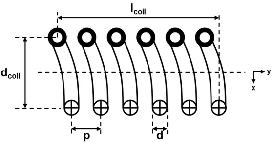
The solenoid design gives the best efficiency (Hoult and Richards, 1976). Solenoid-shaped coils have thus been extensively used in MRM experiments and all parameter dependencies introduced below are based on a solenoid model. Figure 6 shows a schematic of a solenoid, with notations of typical features. In the following paragraphs, we will detail the origins and implications of each of the factors introduced in Equation (2.4).

Figure 6. Cutaway schematic of a solenoid, showing the main geometric characteristics. The current flows into the page at the bottom and out of the page at the top. The number of turns is n = 6. The solenoid axis is along y. The coil diameter and length are defined

from wire center to wire center and are labeled dcoil and lcoil, respectively. The wire

diameter is d, and the total wire length is approximately � � _�� _��. The spacing

(36)

35 Signal dependencies

Let us go back to the origin of the received NMR signal and consider the transverse (i.e. rotating) component of the magnetization, Mxy(r), in an elementary volume V. According to Faraday’s law, the changing magnetic flux associated with the magnetic moment (Mxy(r)* V) will induce a voltage U across the receiver coil. The principle of reciprocity relates U directly to the strength of the magnetic field produced in the transverse plane Bxy(r) by a unit current flowing in the coil at the Larmor frequency (Hoult and Richards, 1976). Thus:

⃗ ⃗ (2.6)

As seen in the introductory part on MRI, the nuclear polarization fraction M0, and therefore Mxy(r), scale linearly with the magnetic field strength B0. The Larmor frequency 0 is also proportional to B0. Thus the voltage induced and thereby the signal received are proportional to the square of the field strength.

(2.7)

Equation (2.6) shows that the signal received is also proportional to the sensitivity of the receiver coil, and using the derivation of the magnetic field inside a solenoid, it has been demonstrated that the field in the very center depends on the geometrical characteristics of the coil via:

√

(2.8)

where 0 is the vacuum permeability and coil parameters are as defined in Figure 6 (Minard and Wind, 2001b). Since the geometric characteristics of the coil also impact the coil resistance and the uniformity of the RF field inside the coil, global recommendations for coil geometry will be provided in more detail in the forthcoming “microcoil” section.

Noise dependencies

Noise in MRI is mainly of thermal origin, arising from Brownian motion of electrons in a conductor, which causes random electrical fluctuations. The corresponding noise power spectral density is 4kBTR, where kB is Boltzmann’s constant, T the absolute temperature and R the conductor resistance. The proposed analysis of the elements

(37)

36

contributing to thermal noise in an NMR experiment is based on work by (Minard and Wind, 2001a). In a “receiver + sample” system, the various elements in which dissipation mechanisms occur are the coil, the leads, the tuning capacitor and the sample. They can each be represented by a separate resistor. Losses in the matching capacitor are negligible when operating near the circuit’s resonant frequency. Thus:

(2.9)

For microscopy size coils (dcoil < 2 mm), noise from the coil is considered to dominate if loaded with biological samples of normal conductivity (Cho et al., 1988; Glover and Mansfield, 2002). However, losses in the tuning capacitor and in the sample increase more rapidly with frequency than losses in the coil, and at frequencies higher than 500 MHz (11.7 T for proton), they cannot be fully neglected.

A solenoid dissipates energy through two processes: eddy currents in the core of the wire that effectively only allow conduction at the wire surface (skin effect), and eddy currents induced in each turn by neighboring turns once the wire is coiled (proximity effect). The skin effect is more pronounced with increasing frequency f, since the current is only carried within a skin depth √ ⁄ , where is the electrical resistivity and r the relative permeability of the conductor (Jackson, 1975). Considering copper at room temperature, the skin depth is for example about 3 µm at 500 MHz and ever thinner with higher frequencies. In this high frequency regime, is therefore much smaller than the wire diameter d, so the resistance of the solenoid due to its sole wire length l can be approximated by:

√ (2.10)

In the high frequency regime (d >> ), the proximity effect results in a coil resistance which is the product of Rwire and an enhancement factor (Butterworth, 1926). The enhancement factor depends on the ratios of coil length to coil diameter and wire diameter to wire spacing. Values of for solenoids with many turns (n > 30) are reported in a table by (Medhurst, 1947) and the enhancement for coils with a lower number of turns n can be approximated by ⁄ . Eventually, at the resonance frequency:

(38)

37

√ (2.12)

The dependencies of the solenoid inductance on geometry are dominated by:

(2.13)

Moving on to the tuning capacitor, its resistance can be written as:

(2.14)

where Ctune is its capacitance and Qcap its quality factor. The latter typically has a frequency dependence that varies with capacitor design. Overall, for a fixed capacitance, capacitor losses can increase with frequency faster than coil losses. Last but not least, a conducting sample will dissipate additional electromagnetic energy in the form of magnetic (m) and dielectric (e) losses: .

Magnetic losses result from the eddy currents induced in the sample by the alternating RF field. Using previous notations and introducing a cylindrical conducting sample of direct current conductivity , the effective resistance associated with magnetic losses is described as follows (Cho et al., 1988):

(2.15)

For samples of large diameter, the total resistance in the system is considered to be dominated by Rm. For the small objects of interest in MRM, the latter is on the contrary usually negligible.

Dielectric losses in aqueous solutions arise from two effects of the alternating electric field: the first is realigning the electric dipoles of water molecules, and the second is moving ions back and forth in the fluid. The latter is a function of sample conductivity and is the dominating source of dielectric losses in biological samples for frequencies below 2 GHz. The exact estimation of Re is not straightforward, with required experimental measurement of certain factors. However, in terms of relative weight compared to other sources of noise, dielectric losses can be quite severe and should not be neglected unless counteracted by special designs (Faraday screen or

(39)

38

distribution of the tuning capacitance throughout the coil structure). For high frequencies:

(2.16)

Overall, if a, b and c are the relative weights of each source of noise (coil+leads, capacitor and sample, respectively) defined by circuit design, temperature and sample conductivity and size, the frequency (and therefore static field) dependence of the equivalent system resistance is:

⁄ (2.17)

where x depends specifically on capacitor model but can be larger than unity. Combining Equations (2.7) and (2.17), the overall impact of magnetic field strength on SNR can be expressed as follows:

√ ⁄ (2.18)

In MRI of large samples, the noise is usually dominated by magnetic losses in the sample, hence SNR α B0. In MRM, there is great incentive in designing the coil and circuit such that the noise is dominated by resistive losses in the coil (SNR α B07/4) but the effective dependence is usually somewhere between B0 and B07/4 due to unavoidable capacitor losses and dielectric losses in the sample. Figure 7 illustrates Figure 7. Relative SNR per unit sample volume as a function of frequency and coil size.

The dashed line represents the ideal ω07/4 response if coil losses dominate, the bold line

shows the limit when either capacitor losses (A) or dielectric sample losses (B: = 1 S/m) dominate. Overall, the SNR performance is significantly degraded by dielectric losses in the sample, and the degradation increases with coil size. From (Minard and Wind, 2001a).