HAL Id: halshs-00575015
https://halshs.archives-ouvertes.fr/halshs-00575015
Preprint submitted on 9 Mar 2011
HAL is a multi-disciplinary open access
archive for the deposit and dissemination of
sci-entific research documents, whether they are
pub-lished or not. The documents may come from
teaching and research institutions in France or
L’archive ouverte pluridisciplinaire HAL, est
destinée au dépôt et à la diffusion de documents
scientifiques de niveau recherche, publiés ou non,
émanant des établissements d’enseignement et de
recherche français ou étrangers, des laboratoires
Existence and stability of overconsumption equilibria
Grégory Ponthière
To cite this version:
WORKING PAPER N° 2009 - 38
Existence and stability of
overconsumption equilibria
Grégory Ponthière
JEL Codes: E13, E21, I12
Keywords: Longevity, growth, overconsumption, obesity,
OLG model
PARIS
-
JOURDAN SCIENCES ECONOMIQUES
LABORATOIRE D’ECONOMIE APPLIQUÉE - INRA
48,BD JOURDAN –E.N.S.–75014PARIS TÉL. :33(0)143136300 – FAX :33(0)143136310
www.pse.ens.fr
Existence and Stability of Overconsumption
Equilibria
Gregory Ponthiere
October 6, 2009
Abstract
Growth models with endogenous mortality assume generally that life expectancy is increasing with output per capita, and, thus, with individ-ual consumption, whatever the consumption level is. However, empirical evidence on the e¤ect of overconsumption and obesity on mortality tends to question that postulate. This paper develops a two-period OLG model where life expectancy is a non-monotonic function of consumption. The existence, uniqueness and stability of steady-state equilibria are studied. It is shown that overconsumption equilibria - i.e. equilibria at which con-sumption exceeds the level maximizing life expectancy - exist in highly productive economies with a low impatience. Stability analysis highlights conditions under which there exist non-converging cycles in output and longevity around overconsumption equilibria.
Keywords: longevity, growth, overconsumption, obesity, OLG model. JEL codes: E13, E21, I12.
1
Introduction
Growth theory has recently paid a particular attention to the study of the rela-tionship between economic development and survival conditions. Following the pioneer works of Blackburn and Cipriani (2002), Chakraborty (2004) and Galor and Moav (2005), various models have been built to explore how accumulation
mechanisms interact with survival conditions.1
Although those models di¤er on signi…cant grounds, a major common feature concerns the modelling of the two-directional relation between economic growth and survival conditions. In those models, longevity a¤ects accumulation deci-sions (e.g. savings, schooling) through a horizon e¤ect: better survival prospects make agents accumulate more, which is bene…cial for the long-run equilibrium of the economy. But those models highlight also the existence of a feedback e¤ect, from economic development to survival conditions. In general, that feedback mechanism takes a simple, monotonic form: economic growth is assumed to raise longevity through a survival function that is increasing in human capital
PSE, Ecole Normale Superieure, Paris. Address: ENS, Department of Social Sciences, boulevard Jourdan, 48, building B, 75014 Paris, France. Contact: [email protected]
1See Bhattacharya and Qiao (2005), Cervallati and Sunde (2005), Chakraborty and Das
or in physical capital (through public and/or private health spending). Hence,
in those models, a higher output leads necessarily to a higher life expectancy.2
The assumption of a monotonic in‡uence of output on survival conditions has two major advantages. On the one hand, it is an analytically convenient way to allow for the endogenization of mortality. On the other hand, this postulate is, at least as a …rst approximation, in line with the available historical trends
showing a positive correlation between consumption and longevity over time.3
However, there are some reasons to question the monotonicity postulate. Those reasons have to do with one of its corollaries, concerning the longevity / consumption relation. Actually, existing models predict that longevity must be increasing monotonically with consumption. The problem is that this is not fully compatible with the data. If one adopts a cross-sectional perspective and plots the levels of consumption and life expectancy across countries, it is easy to see that the relationship between the two variables is far from monotonic. As shown by the tendency curve drawn on Figure 1, life expectancy at birth is increasing with consumption per capita only up to some level of consumption,
but, beyond that level, life expectancy is declining in consumption.4
72 74 76 78 80 82 84 7500 12500 17500 22500 27500 32500 37500 consumption per capita, 2006 (US$)
li fe exp ectanc y at b irth , 2006 (years)
Figure 1: Consumption per head and life expectancy at birth, 2006.
Obviously, Figure 1 is not a proof of the non-monotonicity of the relation un-der study: the non-linear relationship may actually hide the in‡uence of omitted variables correlated with consumption and in‡uencing life expectancy in a non-monotonic way. Nevertheless, Figure 1 has a strong corollary for the modelling of longevity in models where survival functions have a single input. Clearly, Figure 1 suggests that if one wants, on the grounds of analytical tractability, 2One exception is Jouvet et al (2007), where production-related pollution reduces longevity. 3In particular, economic historians emphasized the link between survival conditions and
economic development through a larger food consumption (see Fogel, 1994, 2004).
4The countries of Figure 1 are: Australia, Austria, Belgium, Canada, Czech Republic,
Fin-land, France, Germany, Greece, Hungary, IceFin-land, IreFin-land, Italy, Japan, Luxemburg, Mexico, New Zealand, Netherlands, Norway, Poland, Portugal, Slovakia, South Korea, Spain, Sweden, Switzerland, Turkey, the United Kingdom, and the United States. Consumption statistics (in US$ with current PPPs) are from the OECD (2009). Period life expectancy statistics (average for both sexes) are from the World Health Organization (2009).
to keep a survival function with a unique input (either consumption or another variable correlated with it), the monotonicity postulate is hard to justify.
Beyond the incapacity of monotonic survival functions to …t aggregate data, the monotonicity postulate can also be questionned in the light of the large
epi-demiological literature on the negative e¤ects of overconsumption on survival.5
Epidemiological studies emphasized a non-monotonic relationship between the body mass index and mortality risks. Under the - quite mild - postulate of a link between food consumption and the body mass index, it is straigthfoward to deduce that more consumption is not necessarily better for health and survival. Although more consumption is good for health up to some level, excessive con-sumption becomes health deteriorating, and may undermine survival prospects. As a reaction to the growing literature on the e¤ects of obesity and
overcon-sumption, the economics of obesity has developed rapidly.6 That emerging …eld
has, among other things, studied the economic determinants of obesity, such as the secular fall of food prices induced by technological progress (see Lak-dawalla and Philipson, 2002). Moreover, it has also questionned the capacity of agents to anticipate the e¤ects of their consumption choices on future health,
and proposed several behavioural theories aimed at explaining obesity.7
Despite the expanding literature on overconsumption, there has been so far no attempt, within growth theory, to account for the non-monotonic relationship between consumption and survival prospects. Existing models made survival depend monotonically on a variable correlated positively with consumption, e.g. (physical or human) capital. But such a simpli…cation may not be benign for the dynamics of output and mortality. The monotonicity assumption, although analytically convenient, may truncate the long-run dynamics of the economy.
The goal of this paper is precisely to study the dynamics of longevity and production in an economy where survival prospects depend on consumption in a non-monotonic manner. For that purpose, we develop a two-period OLG model with physical capital accumulation, largely in line with Chakraborty’s (2004) seminal paper. However, a major di¤erence with respect to Chakraborty’s model is that, in our economy, life expectancy is increasing with …rst-period consump-tion up to some "healthy" consumpconsump-tion level, but starts declining for higher consumption levels. As a consequence of this, life expectancy is no longer in-creasing monotonically with physical capital (unlike in Chakraborty’s model).
In economies with a large production capacity, the long-run equilibrium may involve some overconsumption, i.e. a consumption exceeding the level that max-imizes survival prospects. That possibility was excluded in existing models, which relied on the "more is always better" postulate. In contrast, this paper pays a particular attention to the conditions guaranteeing the existence of over-consumption equilibria. A strong emphasis will also be laid on the stability of those equilibria. Can there be stable overconsumption equilibria? Or should we expect non-converging cycles to occur? This paper proposes to cast a new light on the existence and stability of overconsumption equilibria.
5See Solomon and Manson (1997), Bender et al (1998), Fontaine et al (2003), Breeze et
al (2005) and Adams et al (2006). The latter study, which focused on a sample of more than 61,000 sub jects, estimated that overweight persons exhibit a risk of death that is between 20 and 40 % higher than the one faced by normal persons. Moreover, obese persons exhibit a risk of death that is between two and three times higher than the norm.
6See the survey of Philipson and Posner (2008). 7See, for instance, Cutler et al (2003).
The rest of the paper is organized as follows. The model is presented in Section 2. Section 3 examines the existence, uniqueness and stability of steady-state equilibria. Section 4 illustrates the dynamics of production and longevity on the basis of numerical simulations. Section 5 concludes.
2
The model
Let us consider a two-period OLG model. For simplicity, we assume that repro-duction is monosexual, and that each person gives birth to exactly one child.
The …rst period is a period of young adulthood, during which the adult gives birth to a child, supplies his labour inelastically and saves some resources for the old age. The second period is a period of retirement.
Survival conditions Only a fraction t+1 of a cohort born at time t
reaches the retirement age.8 The fraction
t+1 depends on the consumption
when being young ctin a non-monotonic way. There exists a level of
consump-tion c that brings the maximum survival probability, i.e. 1. Any departure from c , either from below or from above, generates a lower survival probability. For simplicity, the probability of survival to the old age is determined by the following survival function
t+1=
1
1 + (c ct)2
(1)
where c > 0 is the "healthy" consumption level, that is, the consumption
level that yields the maximum life expectancy. The parameter 0 captures
the impact of consumption on survival prospects. Note that limct!0 t+1 =
1
1+ c 2 , which is close to zero when the healthy consumption level c is
high. Moreover, we have that limct!c t+1= 1 and limct!1 t+1= 0.
consumption su rvi val p ro b ab il ity Figure 2: t+1as a function of ct
Figure 2 illustrates the relationship between t+1and ct.9 When
consump-tion is inferior to the healthy consumpconsump-tion level c , a higher consumpconsump-tion raises
survival prospects. On the contrary, if ct > c , the opposite prevails: a lower
consumption would raise life expectancy.
8Hence the life expectancy at birth of cohort t is here equal to 1 + t+1. 9On Figure 1, we have c = 30, and = 0:005.
Production Firms at time t produce some output Yt according to the
production function Yt = F (Kt; Lt), where Ktdenotes the total capital stock,
and Lt denotes the labour force. For simplicity, F (:) takes the Cobb-Douglas
form:
Yt= AKtL1t (2)
where 0 < < 1 and A > 0. We assume also a full depreciation of capital after
one period of use.
In intensive terms, the production process can be rewritten as
yt= Akt (3)
where ktis the capital per worker.
Factors are paid at their marginal productivities:
Rt = Akt 1 (4)
wt = (1 )Akt (5)
where Rtis 1 plus the interest rate, while wtis the wage rate.
The savings decision Each young adult at time t makes a single decision:
the amount he saves for his old days (i.e. st), and, as a consequence of his budget
constraint, his consumption when being young ct.
For analytical convenience, it is also assumed, as in Chakraborty (2004), that a perfect annuity market exists, which yields an actuarially fair return.
Under logarithmic temporal utility, and provided the utility of being dead is normalized to zero, the problem of each young adult is to maximize
log (wt st) + et+1log
Rt+1st
e t+1
(6)
where is a time preference factor (0 1), while e
t+1 is the subjective
probability of survival to the second period.
The actual survival probability to the old age depends on the consumption when being young. However, to be in line with the microeconomics of obe-sity and overconsumption, it is assumed here that the agent does not, when he chooses his consumption pattern, internalize the impact of his choice on his sur-vival prospects. On the contrary, the agent takes the future sursur-vival prospects as given, and thus independent from his behaviour. Agents’decisions are assumed
to be based on myopic anticipations about t+1 (i.e. et+1= t).
The …rst-order condition for optimal savings yields
st= t
1 + t
wt (7)
As usual, savings is increasing with the expected lifetime of the agent.10
1 0Under a full anticipation of the impact of consumption on survival, we would have:
st 2 41 + log Rt+1st t+1 0(ct) ct 1 + t+1 3 5 = t+1 1 + t+1 wt
3
Steady-state equilibria
Let us now study the long-run dynamics of the economy. Given the replace-ment fertility and the full depreciation of capital, the capital market equilibrium condition is
kt+1= st (8)
Hence, by substituting for the wage into optimal savings, one has:
kt+1= t
1 + t
A(1 )kt
Obviously, if kt = 0, we have kt+1 = 0, whatever t is. Hence, in the
( t; kt) space, the kk locus, that is, the combinaisons of ktand t such that kt
is constant over time, includes the horizontal axis, i.e., all points ( t; 0).
Imposing kt+1= kt 6= 0 gives the other part of the kk locus:
kt= t A(1 ) 1 + t 1 1 G( t) (9)
We have G(0) = 0, G0( t) > 0 and G(1) < 1. Figure 3 illustrates the kk locus
in the ( t; kt) space.11 Under kt> 0, the sustainable level of capital is unique,
and is increasing in t: the higher the life expectancy 1 + t is, the higher the
sustainable level of capital is. Levels of kthigher than the kk locus cannot, given
the prevailing survival conditions, be reproduced over time. Inversely, levels of capital lower than the kk locus lead to a larger capital at the next period (as a high life expectancy implies here a large propensity to save).
probability of survival ca p ital p e r w o rker kk locus
Figure 3: The kk locus
Figure 3 illustrates the relation between the time horizon of agents and the sustainable level of capital. In particular, for bad survival conditions (i.e. a low
t), only extremely low capital levels can be reproduced over time.
is equal to the previous one only if consumption does not a¤ect survival prospects: 0(ct) = 0.
However, if t+1depends on consumption, that derivative is not zero. Clearly, if ctis below
(resp. above) c , we have 0(ct) > 0(resp. 0(ct) < 0), so that the agent tends to save too
much (resp. too little) - and to consume too little (resp. too much) in the …rst period - with respect to what maximizes his lifetime welfare.
Let us now derive the locus, that is, the combinaisons of kt and tsuch
that tis constant over time. From the survival function, we have
t+1=
1
1 + c 1+1
tA(1 )kt
2
Imposing t+1 = t gives the locus. Because of the squared bracket at
the denominator of the survival function, there exists, in general, not one, but
two levels of capital that maintain tat a constant level. These are given by:
kt = " c 1 1=2 1 t t 1=2! 1 + t A(1 ) #1 H1( t) (10) kt = " c + 1 1=2 1 t t 1=2! 1 + t A(1 ) #1 H2( t) (11)
If t= 1, then H1(1) = H2(1), as there is a unique level of capital that makes
t constant at its maximal level, and that level of kt is such that consumption
equals c . For 0 t < 1, we have H2( t) > H1( t). Hence, we shall call
H1( t) the low branch of the locus, and H2( t) the high branch of the
locus. Those two branches intersect only at t= 1.
Regarding the shape of H1( t), we have lim t!0H1( t) = 1 if 1= is
odd, and lim t!0H1( t) = +1 if 1= is even.
12 Moreover, if 1= is odd, we
have H10( t) > 0 for any t. On the contrary, for 1= even, we have H10( t) < 0
for t < and H10( t) > 0 for t > , where = 1+ c1 2. Note also that, if
t=1+ c1 2 , then H1( t) = 0.
As far as H2( t) is concerned, we have lim t!0H2( t) = +1. Moreover,
we have H20( t) < 0 for any tsuch that
1 12 1 t t 1 2 1 2 (1 + t) t(1 t) > c If t< , we have 1 1 2 1 t t 1 2
> c . Hence, given that the term in brackets
lies in the interval [2; +1], it must be the case that H0
2( t) < 0: Alternatively, if t> , we have 1 1 2 1 t t 1 2
< c , and so it may be the case that H20( t) > 0:
Figures 4a and 4b illustrate the form of the locus in the ( t; kt) space.13
For t < 1, there exists an interval of levels for capital per worker that
al-low a growth of life expectancy over time. That interval lies between the two
branches of the locus. Levels of kt outside that interval lead to a fall of
life expectancy. Such a fall can arise either because kt is too low (bottom of
the phase diagram), or because kt is too high (top of the phase diagram). In
the former case, consumption is lower than the level that would maintain life
expectancy unchanged. As a consequence, tmust fall, as only a lower survival
probability can be sustained for such a low consumption level. In the latter 1 2See the Appendix.
1 3On Figure 4a, we have A = 25, = 0:30, = 0:40, c = 20 and = 0:01:Same values on
case, a fall of t arises because kt is too high: consumption exceeds the level
that would maintain tconstant, explaining the fall of t.
probability of survival ca p ital p e r w o rker pp locus (H1) pp locus (H2)
Figure 4a: The locus (1= is odd)
probability of survival ca p ital p e r w o rker pp locus (H1) pp locus (H2)
Figure 4b: The locus (1= is even)
The di¤erence between Figures 4a and 4b concerns the shape of the locus
in the neighbourhood of t= 0. In Figure 4a, where 1= is odd, the low branch
of the locus tends to 1 as ttends to 0, whereas, in Figure 4b, where 1=
is even, the low branch of the locus tends to +1 as t tends to 0.
There can be three distinct kinds of stationary equilibria in the economy under study, as the intersections of the two loci can occur either on the low
branch of the locus, or on the high branch of the locus, or at the
inter-section of the two branches, i.e. at t= 1. In the rest of this paper, we will coin
the di¤erent types of equilibria as follows. The …rst type of intersection will be called an underconsumption equilibrium, as consumption at such an equilib-rium is below the healthy consumption level c . The second type of equilibequilib-rium will be referred to as an overconsumption equilibrium, as consumption exceeds c at that equilibrium. The third type of intersection will be called a healthy
consumption equilibrium, as we have ct= c at that equilibrium.
Let us now use the properties of the kk locus and the locus to study the
existence of steady-state equilibria. Proposition 1 summarizes our results.
Proposition 1 Let us denote G(1) by k h A(11+ )i
1 1 and H1(1) = H2(1) by hc A(11+ )i 1 :
(1) If 1 is odd and ifh A(11+ )i
1 1
< , there exist at least two
undercon-sumption steady-state equilibria: ( ; 0) and ( 1; k1), with 0 < < 1 < 1 and
0 < k1< k :
(2) If 1 is odd and ifh A(11+ )i
1 1
> , there exist at least one
undercon-sumption steady-state equilibrium ( ; 0) and one overconundercon-sumption steady-state
equilibrium ( 2; k2), where 0 < 7 2< 1 and 0 < k < k2:
(3) If 1 is odd and ifh A(11+ )i
1 1
= , there exist at least one
undercon-sumption steady-state equilibrium ( ; 0) and exactly one healthy conundercon-sumption steady-state equilibrium (1; k ).
(4) If 1 is even and ifh A(1 ) 1+
i 1
1
< , there exists at least three
under-consumption steady-state equilibria ( ; 0), ( 3; k3) and ( 4; k4), with 0 < 3<
< 4< 1 and 0 < k3< k4< k :
(5) If 1 is even and if h A(11+ )i
1 1
> , there exists at least two
under-consumption steady-state equilibria ( ; 0) and ( 5; k5), and at least one
overcon-sumption equilibrium ( 6; k6), with 0 < 5< , 7 6< 1 and 0 < k5< k <
k6.
(6) If 1 is even and if h A(1 )
1+
i 1
1
= , there exists at least two
under-consumption steady-state equilibria ( ; 0) and ( 7; k7), and exactly one healthy
consumption equilibrium (1; k ), with 0 < 7< < 1 and 0 < k7< k .
Proof. See the Appendix.
Proposition 1 states that the minimal number of steady-state equilibria
de-pends on the structural parameters of the economy.14 In cases (4) to (6), where
1= is even, there must exist a stationary equilibrium in the left corner of the
( t; kt) space, because the low branch of the locus is decreasing for levels
of t inferior to , unlike what prevails under cases (1) to (3), where 1= is
odd. This is the reason why cases (4) to (6) admit a higher minimal number of steady-state equilibria than cases (1) to (3).
Regarding the distinction between, on the one hand, cases (1) and (4), and, on the other hand, cases (2) and (5), this lies in the types of steady-state
equi-libria that exist in each case. The stationary equiequi-libria ( ; 0), ( 1; k1), ( 3; k3),
( 4; k4) and ( 5; k5) are underconsumption equilibria, i.e. equilibria located
on the low branch of the locus. On the contrary, ( 2; k2) and ( 6; k6) are
overconsumption equilibria, i.e. equilibria located on the high branch of the locus. While this constitutes a signi…cant di¤erence, this does not allow us, however, to deduce whether life expectancy is higher at an underconsumption equilibrium or at an overconsumption equilibrium, as the level of life expectancy depends on the distance between consumption and healthy consumption.
Overconsumption equilibria ( 2; k2) and ( 6; k6) are, ceteris paribus, more
likely to prevail in economies with a higher productivity (i.e. with a high A). Similarly, it is clear, from Proposition 1, that overconsumption equilibria are
more plausible in economies where the time preference factor is close to unity.
Under a low impatience, we have G(1) > H1(1) = H2(1), which leads to an
overconsumption equilibrium. Finally, economies where the healthy consump-tion level c is, because of external reasons, lower are also more likely to exhibit an overconsumption equilibrium.
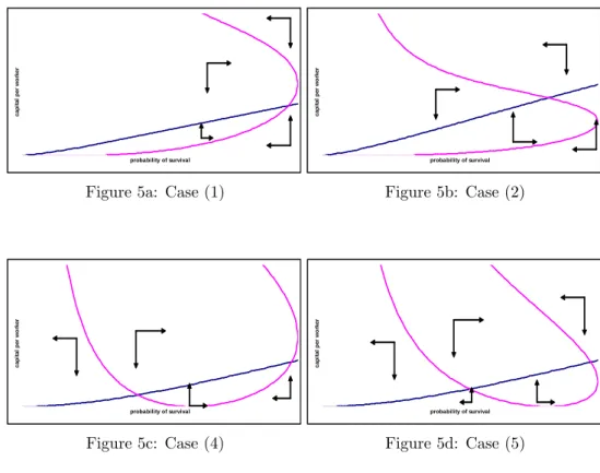
Cases (1), (2), (4) and (5) of Proposition 1 are illustrated on Figures 5a to
5d, which show the kk locus and the locus in the ( t; kt) space.15 In order
to give us some clues regarding the local stability of stationary equilibria, those …gures exhibit dynamic arrows, showing the direction of change over time. In 1 4Proposition 1 concerns only the minimal number of equilibria because the existence proof
relies on the limits of the functions G( t), H1( t)and H2( t)for ttending towards 0 and
1. Additional assumptions on the second-order derivatives of the loci are needed to be able to make statements about the actual number of intersections of the two loci (see the Appendix).
1 5On Figure 5a, we have A = 20, = 0:30, = 0:40, c = 20, and = 0:01. On Figure 5b,
we have A = 25, = 0:30, = 0:40, c = 20, and = 0:01. On Figure 5c, we have A = 25, = 0:50, = 0:40, c = 20, and = 0:001. On Figure 5d, we have A = 20, = 0:50, = 0:40, c = 15, and = 0:001:
each case, there exists a vast area of the ( t; kt) space where both capital per worker and life expectancy are growing. Note, however, that the size of that area varies strongly across the cases. More importantly, the extent to which an
economy with initial conditions ( 0; k0) can end up in that area varies across
cases. Under cases (4) and (5), there exists a large area, in the bottom left corner of the phase diagram, where both capital per worker and life expectancy are falling. In those cases, the intermediate equilibrium is unstable, and acts like a threshold, below which economies are condamned to stagnate, with low output, consumption and life expectancy.
probability of survival cap it al p e r wo rker
Figure 5a: Case (1)
probability of survival cap it al p e r wo rker Figure 5b: Case (2) probability of survival cap it al p e r wo rker Figure 5c: Case (4) probability of survival cap it al p e r wo rker Figure 5d: Case (5)
Whereas this discussion gives us some clues about the instability of some equilibria, it should be reminded, however, that a mere look at a phasis diagram does not su¢ ce to provide accurate results on the stability of equilibria. For instance, on Figure 5b, it is not possible to see, on the mere basis of graphical analysis, whether the equilibrium is stable or not: even though the dynamic arrows seem to point to the equilibrium, nothing insures the actual convergence to that equilibrium. Hence a formal analysis of stability is required.
Such an analysis is carried out in the Appendix of this paper. Proposition 2 summarizes our results.
The conditions (1 + )h1 + (c c)2i 2 h 2 (c c) 1+c i h1 + 1+ i h 1 + (c c)2i2 > 0 (1 )h1 + (c c)2i2+h2 (c c) 1+c i h1 1+ i h 1 + (c c)2i2 > 0 h 1 + (c c)2i2+ 2 (c c)c h 1 + (c c)2i2 > 0
are necessary and su¢ cient for the local stability of that equilibrium.
Proof. See the Appendix.
Those conditions concern the local stability only, and not the global sta-bility, because, as this was shown above, there exist, in each of the cases (1) to (6), at least two steady-state equilibria, so that no condition can guarantee an unconditional convergence towards an equilibrium for any initial conditions
( 0; k0).
The stability conditions stated in Proposition 2 depend on the magnitude
of the parameter , which captures the sensitivity of life expectancy to the
consumption behaviour. Clearly, if tends to 0, the stability conditions of
Proposition 2 become respectively 1 + > 0, 1 > 0 and 1 > 0, which are
all true given our assumption 0 < < 1. However, larger values of make the
local stability of the stationary equilibrium less likely.
The stability conditions of Proposition 2 are general, and, as such, are not
simple to interpret.16 In order to have a more concrete idea of the conditions
under which stability prevails, let us now focus on the case of an overconsump-tion equilibrium. It can be shown that, for overconsumpoverconsump-tion equilibria, such as
( 2; k2) and ( 6; k6), a simple condition guarantees local stability.
Proposition 3 The condition
2 (c c) c1+
h
1 + (c c)2i
2 < 1
is su¢ cient for the local stability of equilibria ( 2; k2) and ( 6; k6).
Proof. See the Appendix.
A lower elasticity of output with respect to capital favours, ceteris paribus,
the stability of the equilibrium. Moreover, the closer the equilibrium consump-tion is to the healthy consumpconsump-tion c , the lower the second term is, making local
stability more plausible. Here again, larger values of make the local stability
1 6One exception concerns the stability of the steady-state equilibrium ( ; 0). Indeed in that
case c = 0 and it is straigthforward to see that the three conditions of Proposition 2 are satis…ed, so that local stability prevails.
of the equilibrium less likely. Finally, the time preference parameter is also present in the stability condition. The more impatient agents are (i.e. a lower
), the lower the second term is, making stability more plausible.17
Let us conclude this stability analysis by considering the possibility of
long-run cycles in the ( t; kt) space. That question can be formulated as follows:
will economies converge, in the long-run, towards unique levels of output and life expectancy, or, on the contrary, will economies exhibit cycles around those steady-states?
As stated in Proposition 4, it is only in the presence of an overconsumption equilibrium, that is, in cases (2) and (5) of Proposition 1, that long-run cycles
can arise in the ( t; kt) space. Such cycles are both economic cycles (i.e. in terms
of capital, output and consumption) and demographic cycles (i.e. in terms of life expectancy and population size). The existence of long-run cycles is subject to some speci…c conditions on the structural parameters of the economy.
Proposition 4 There exists no long-run cycle around steady-state equilibria
( ; 0), ( 1; k1), ( 3; k3), ( 4; k4), ( 5; k5), ( 7; k7) and (1; k ).
There exist long-run cycles around the steady-states ( 2; k2) and ( 6; k6) if
and only if the following conditions are satis…ed:
(i) [1+ (c c) 2 ]2 2 (c c)( c 1+ ) [1+ (c c)2]2 2 + 8 (c c)( c 1+ )(1+ 1 ) [1+ (c c)2]2 < 0 (ii) 2 r 2 (c c)( c 1+ )(1+ 1) [1+ (c c)2]2 = 1
where and c take their equilibrium values.
Proof. See the Appendix.
It is easy to see why cycles cannot arise around underconsumption equilibria
like ( ; 0), ( 1; k1), ( 3; k3), ( 4; k4) or ( 5; k5). Indeed, in those cases, the
condition (i) is necessarily violated, as c < c . It is thus only at overconsumption
equilibria, like ( 2; k2) and ( 6; k6), that condition (i) can be satis…ed, and if
condition (ii) is also true, then a cycle exists around the steady-state.
Note, here again, the crucial role played by the parameter . If is close
to zero, cycles cannot occur, as conditions (i) and (ii) are necessarily violated. Moreover, for too high levels of , it is condition (ii) that would not be satis-…ed: the economy would just diverge in the long-run, without exhibiting a cycle. Thus, the existence of long-run cycles requires a particular set of conditions, in-cluding a sensitivity of life expectancy to consumption behaviour that is neither too small, neither too large.
While Proposition 4 informs us about the general conditions under which
long-run cycles exist in the ( t; kt) space, it is di¢ cult to know a priori whether
conditions (i) and (ii) are strong or weak, and whether these are compatible with standard values for the parameters of the economy. The task of the next section is to discuss this by means of numerical simulations.
4
Numerical illustrations
This Section illustrates numerically the dynamics of production and longevity in the economy under study. For that purpose, we will concentrate here on 1 7The intuition behind this lies in the mere fact that, if is low, the agent’s reactions to a
the cases of advanced economies, i.e. on economies with a high productivity. Hence, the equilibria under study belong here to the cases (2) and (5) of
Propo-sition 1 (i.e. steady-states ( 2; k2) and ( 6; k6)). We will rely on the following
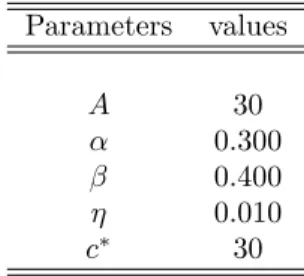
benchmark values for the structural parameters of the economy.18
Parameters values A 30 0.300 0.400 0.010 c 30
We shall also take, as initial conditions, k0= 0:1 and 0= 0:05 (for periods
of 30 years, this coincides with an initial life expectancy of about 61.5 years).
It is easy to check that, under those parameters values, we havehc A(11+ )i
1 < h A(1 ) 1+ i 1 1
, so that, given 1= odd, we are in case (2).
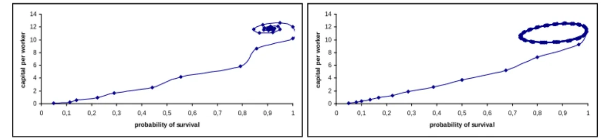
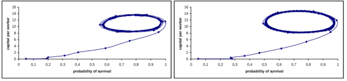
In the light of the discussions in Section 3, one can expect that the dynamics of production and longevity depends on the parameter , which determines the reaction of longevity when consumption departs from its healthy level. Those intuitions are con…rmed by Figures 6a-6d, which show the dynamics of the
economy in the ( t; kt) space. Under low values of , the convergence to the
long-run equilibrium is monotonic, except when the economy is very close to the long-run equilibrium (see Figures 6a and 6b). A converging spiral holds
under = 0:020 (Figure 6c). However, under = 0:030 (Figure 6d), there is a
non-converging cycle, as the economy satis…es the conditions of Proposition 4.
0 2 4 6 8 10 12 14 0 0,1 0,2 0,3 0,4 0,5 0,6 0,7 0,8 0,9 1 probability of survival cap ital p er wo rker Figure 6a: = 0:005 0 2 4 6 8 10 12 14 0 0,1 0,2 0,3 0,4 0,5 0,6 0,7 0,8 0,9 1 probability of survival cap ital p er wo rker Figure 6b: = 0:010
1 8Note that the time preference parameter , which is …xed to 0:40, is slightly larger than
the usual value of 0:30. Actually, 0:30 is generally used, as this coincides with a quarterly discount factor of 0:99. Here we rely on a higher value for , as there is already some "natural" discounting through the survival probability.
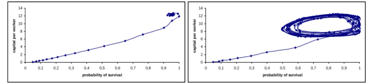
0 2 4 6 8 10 12 14 0 0,1 0,2 0,3 0,4 0,5 0,6 0,7 0,8 0,9 1 probability of survival cap ital p er wo rker Figure 6c: = 0:020 0 2 4 6 8 10 12 14 0 0,1 0,2 0,3 0,4 0,5 0,6 0,7 0,8 0,9 1 probability of survival cap ital p er wo rker Figure 6d: = 0:030
An interesting feature of Figures 6c and 6d is that, if we look at the …rst
10 periods of time, the dynamics is quasi identical whatever equals 0:020 or
0:030. Given the substantial length of each period (equal to about 30 years), it follows from this that empirical evidence covering something like three centuries
of data on output and longevity would not help us to distinguish between =
0:020 and = 0:030, even though the long-run dynamics induced by those two
parametrizations are very di¤erent. This constitutes a quite negative result, as one can thus hardly, on the basis of existing data sets, discriminate between di¤erent levels of , and, hence, detect the possible existence of cycles.
Consumption 0 10 20 30 40 12 3 4 5 6 7 8 9 10 11 12 13 14 15 16 17 18 19 20 21 22 23 24 25 26 27 28 29 30
Figure 7a: the dynamics of consumption
Life expectancy 0 0,5 1 1,5 2 2,5 1 2 3 4 56 7 8 9 10 11 12 13 14 15 16 17 18 19 20 21 22 23 24 25 26 27 28 29 30
Figure 7b: the dynamics of life expectancy
In order to understand the mechanism behind long-run cycles, Figures 7a
and 7b show the time series of consumption and life expectancy under equal to
0:030. As long as consumption is below the healthy consumption level c (equal to 30), the capital accumulation process makes consumption grow towards c , implying a growth of life expectancy. Thanks to the horizon e¤ect, a high life
expectancy keeps on reinforcing capital accumulation, which raises consumption
beyond c . This overconsumption leads to a fall of life expectancy. For a
low level of , departures from c cause only small changes in life expectancy, which will have minor e¤ects on capital accumulation, and, thus, on future
consumption and life expectancy. Hence, for low levels of , there will be a
convergence of ctand ttowards the long-run equilibrium. However, for larger
values of , the fall of life expectancy induced by an excessive consumption
is signi…cant. Due to the horizon e¤ect, that fall of life expectancy reduces capital accumulation, and, in …ne, consumption, which falls down towards its healthy level. This raises life expectancy again, which increases savings and capital accumulation, and so forth. A large , by implying strong upwards and downwards reactions of life expectancy to consumption and vice versa, is thus
the cause of the instability, which takes here the form of a cycle.19
Let us now examine the robustness of those results to the calibration of the other parameters. As shown on Figures 8a-8b, a slight change in the level of healthy consumption c has large e¤ects on the long-run dynamics of longevity
and capital. On Figure 8a, we can see that, under = 0:030, cycles disappear
once c is raised from 30 to 31. On the contrary, Figure 8b shows that cycles become larger once healthy consumption is slightly reduced.
0 2 4 6 8 10 12 14 0 0,1 0,2 0,3 0,4 0,5 0,6 0,7 0,8 0,9 1 probability of survival cap ital p er wo rker Figure 8a: = 0:030; c = 31 0 2 4 6 8 10 12 14 0 0,1 0,2 0,3 0,4 0,5 0,6 0,7 0,8 0,9 1 probability of survival cap ital p er wo rker Figure 8b: = 0:030; c = 29
Beyond and c , other parameters enter the stability condition of
Proposi-tion 3, and can be expected to in‡uence the overall dynamics of the economy.
Take, for instance, the time preference parameter . The higher it is, the
stronger is the horizon e¤ect ceteris paribus, and so the stronger the feedback from capital accumulation to survival conditions is. Note, however, that nu-merical simulations under the benchmark values of the other parameters do not
point to a signi…cant sensitivity of the long-run dynamics to the level of .20
On the contrary, the dynamics of output and longevity is strongly sensitive
to the parameter , i.e. the elasticity of output with respect to capital. This
in‡uence is obvious in the light of the stability condition of Proposition 3: the
higher is, the less plausible local stability is. As shown on Figure 9a, once is
raised to 0.4, a level of as low as 0.008 su¢ ces to bring a non-converging cycle,
whereas, under = 0:5, non-converging cycles appear for = 0:004 (Figure 9b).
1 9Note that larger levels of can lead to diverging spirals around the equilibrium. 2 0But this does not mean that this parameter is benign, as it in‡uences naturally the
position of the steady-state equilibrium levels of output and life expectancy. Because of space constraints, those simulations are not included here.
Hence, more capital-intensive economies are also likely to exhibit an unstable stationary equilibrium. 0 2 4 6 8 10 12 14 16 0 0,1 0,2 0,3 0,4 0,5 0,6 0,7 0,8 0,9 1 probability of survival cap ital p er wo rker Figure 9a: = 0:4; = 0:008 0 2 4 6 8 10 12 14 16 0 0,1 0,2 0,3 0,4 0,5 0,6 0,7 0,8 0,9 1 probability of survival cap ital p er wo rker Figure 9b: = 0:5; = 0:004
Finally, note that, although the productivity parameter A does not explic-itly enter the stability condition in Proposition 2, it tends, however, to have a signi…cant in‡uence on the dynamics of output and longevity. As shown on
Fig-ure 6b, there is, under equal to its benchmark value of 0:01, a non-monotonic
convergence of the economy to the steady-state equilibrium under A = 30. Fig-ures 10a and 10b show that changes in A a¤ect the dynamics signi…cantly: the
convergence becomes monotonic in t and kt under A = 25 (Figure 10a), and
there exists a non-converging cycle under A = 35 (Figure 10b).
0 1 2 3 4 5 6 7 8 0 0,1 0,2 0,3 0,4 0,5 0,6 0,7 0,8 0,9 1 probability of survival cap ital p er wo rker Figure 10a: A = 25 0 2 4 6 8 10 12 14 16 0 0,1 0,2 0,3 0,4 0,5 0,6 0,7 0,8 0,9 1 probability of survival cap ital p er wo rker Figure 10b: A = 35
Hence, more productive economies are more likely to exhibit a cyclical dy-namics than less productive economies. Indeed, in more productive economies, the impact of capital accumulation in terms of output and consumption is larger. As a consequence, the reactions of longevity to capital accumulation are also larger, reinforcing the likelihood of cycles.
That result is worth being stressed, especially if one thinks that a major lim-itation of the model developed in Section 2 lies in the absence of technological progress. Figure 10b suggests that if some exogenous technological progress was
assumed instead (i.e. a variable At A(1 + g)tin the production function), the
high levels of Atreached after some periods of time would lead the economy to
‡uctuations in output and life expectancy. Hence the introduction of some ex-ogenous technological progress would reinforce the likelihood of long-run cycles. However, endogenous technological progress may or may not do so, depending on the precise modelling of the determinants of technological change.
5
Conclusions
The large theoretical literature on the relation between economic growth and longevity gains assumes usually that survival is increasing monotonically with the level of (physical or human) capital, either directly or indirectly (e.g. through health spending). Nevertheless, that postulate has a counterintuitive corollary: survival must, in general, be correlated positively with consumption, whatever the consumption level is. That corollary is not compatible with the epidemio-logical literature showing that excess consumption leads to a larger mortality.
This paper developed a two-period OLG model where the probability of sur-vival to the second period is non-monotonic in consumption, and is increasing in consumption only as long as consumption lies below a healthy consumption level. The study of the existence, uniqueness and stability of steady-state equi-libria revealed that the dynamics of output and longevity varies strongly with the structural parameters of the economy, which can lead to either an overcon-sumption or an underconovercon-sumption equilibrium. The stability of the equilibrium is not guaranteed: cycles may exist around long-run equilibria, in the sense that periods of economic growth and longevity improvement would be followed by periods of economic contraction and lower life expectancy, and so forth.
Long-run economic and demographic cycles exist only around overconsump-tion equilibria, and under particular condioverconsump-tions on the structural parameters of the economy. Cycles are more plausible in economies with a high sensitivity of life expectancy to consumption behaviour, and where, because of exogenous reasons, the healthy consumption level is lower. Cycles are also more likely the more productive and capital-intensive the economy is. Those features are all shared by advanced economies, so that the present …ndings do not allow us to exclude a priori the possibility of future economic and demographic cycles due to the nefast e¤ect of overconsumption on survival conditions.
6
References
Adams, K., Schatzkin, A., Harris, T., Kipnis, V., Mouw, T., Ballard-Barbash, R., Hollenbeck, A. & Leitzmann, M. (2006): "Overweight, obesity, and mortality in a large prospective cohort of persons 50 to 71 years old", The New England Journal of Medicine, 355 (8), pp. 763-778.
Bender, R., Trautner, C., Spraul, M. & Berger, M. (1998): "Assessment of excess mortality in obesity", American Journal of Epidemiology, 147, 1, pp. 42-47.
Bhattacharya, J. & Qiao, X. (2005): "Public and private expenditures on health in a growth model", Iowa State University Working Paper, #05020.
Blackburn, K. & Cipriani, G.P. (2002): "A model of longevity, fertility and growth", Journal of Economic Dynamics and Control, 26, pp. 187-204.
Breeze, E., Clarke, R., Shipley, M., Marmot, M., & Fletcher, A. (2005): "Cause-speci…c mortality in old age in relation to body mass index in middle age and in old age: follow-up of the Whitehall cohort of male civil servants", International Journal of Epidemiology, 35(1), pp. 169-178.
Cervellati, M. and Sunde, U. (2005): "Human capital formation, life ex-pectancy, and the process of development", American Economic Review, 95, pp. 1653–1672.
Chakraborty, S. (2004): "Endogenous lifetime and economic growth", Jour-nal of Economic Theory, 116, pp. 119-137.
Chakraborty, S. and Das, M. (2005): "Mortality, human capital and persis-tent inequality", Journal of Economic Growth, 10, pp. 159–192.
Cutler, D., Glaeser, E. & Shapiro, J. (2003): "Why have Americans become more obese?", Journal of Economic Perspectives, 17(3), pp. 93-118.
de la Croix, D. & Licandro, O. (2007): "The Child is the Father of Man", CORE Discussion Paper 2007-72.
Fogel, R. (1994): "Economic growth, population theory and physiology: the bearing of long-term processes on the making of economic policy", American Economic Review, 84(3), pp. 369-395.
Fogel, R. (2004): "Health, nutrition and economic growth", Economic De-velopment and Cultural Change, 52(3), pp. 643-658.
Fontaine, K., Redden, D., Wang, C., Westfall, A. & Allison, D. (2003): "Years of life lost due to obesity", The Journal of the American Medical Asso-ciation, 289(2), pp. 187-193.
Galor, O., & Moav, O. (2005): "Natural selection and the evolution of life expectancy", CEPR, Minerva Center for Economic Growth Paper 02-05.
Jouvet, P.A., Pestieau, P., Ponthiere, G., (2007): "Longevity and environ-mental quality in an OLG model", CORE Discussion Paper 69.
Lakdawalla, D. & Philipson, T. (2002): "The growth of obesity and tech-nological change: a theoretical and empirical examination", NBER Discussion Paper 8946.
Medio, A. & Lines, M. (2001): Non Linear Dynamics: A Primer. Cambridge University Press.
OECD (2009): OECD Statistics, data retrived on 01/08/2009, at http://stats.oecd.org/index
Philipson, T. & Posner, R. (2008): "Is the obesity epidemic a public health problem? A decade of research on the economics of obesity", NBER Discussion Paper 14010.
Solomon, C. & Manson, J. (1997): "Obesity and mortality: a review of the epidemiological data", The American Journal of Clinical Nutrition, 66(4), pp. 1044-1050.
World Health Organization Statistical Information System - WHOSIS (2009), data retrived on 01/09/2009, at http://apps.who.int/whosis/data/Search
Zhang, J., Zhang, J., & Leung, M.C. (2006): "Health investment, saving, and public policy", Canadian Journal of Economics, 39, 1, pp. 68-93.
7
Appendix
7.1
Proposition 1
The existence of a steady-state equilibrium can be explored as the issue of the
intersection of the kk locus and the locus in the two-dimensional space
( t; kt). For that purpose, let us …rst derive the basic properties of those two
loci.
We know that G(0) = 0 and that, under kt = 0, t is maintained constant
The …rst-order derivative of G(:) is G0( t) = 1 1 [A(1 ) ] 1 1 1 1 1 t 1 1 + t 2 1 > 0 Regarding H1( t), we have lim t!0 H1( t) = " c 1 1=2 1 0 1=2! 1 A(1 ) #1 = 1 if 1= is odd = +1 if 1= is even Moreover H10( t) = 1 " c 1 1=2 1 t t 1=2! (1 + t) A(1 ) #1 1 " 1 1=2 1 2 1 t 1=2(1 )1=2A(1 ) ! + c A(1 ) #
If 1= is odd, (1= ) 1 is even, so that the …rst factor is always positive,
whatever tis. Given that the second factor is always positive (as 1 1t),
we have thus H0
1( t) > 0. However, if 1= is even, (1= ) 1 is odd, so that the
…rst factor is negative for low levels of t< =1+ c1 2, but positive for t> :
Given that the second factor is always positive, we have H0
1( t) < 0 for t<
and H0
1( t) > 0 for t> . At t= , we have H10( t) = 0:
Note also that:
lim t!0 H10( t) = 1 " c 1 1=2 1 0 1=2! 1 A(1 ) #1 1 " 1 2 1 0 1=2 1 1=21 0 1 A(1 ) + c 1 1=2 1 0 1=2! A(1 ) # = +1 if 1= is odd = 1 if 1= is even and lim t!1 H10( t) = 1 c (1 + ) A(1 ) 1 1" 1 2 0 1 1=2 1 1=2 1 + A(1 ) + c A(1 ) # = +1 Regarding H2( ), we have lim t!0 H2( t) = " c + 1 1=2 1 0 1=2! 1 A(1 ) #1 = +1
Moreover, H20( t) = 1 " c + 1 1=2 1 t t 1=2! (1 + t) A(1 ) #1 1 " 1 1=2 12 1=2t (1 + t) + (1 t) 2 t(1 t)1=2A(1 ) ! + c A(1 ) #
The …rst factor is always positive, whatever tis. But the second factor can
be positive or negative, depending on the level of t:Actually, if t< =1+ c1 2,
we always have H0
2( t) < 0, but this may not be the case for t> :
Note also that: lim t!0 H20( t) = 1 " c + 1 1=2 1 0 0 1=2! 1 A(1 ) #1 1 " 1 1=2 1201=2t + 0A(1 ) ! + c A(1 ) # = +1 and lim t!1 H20( t) = 1 " c + 1 1=2 (0)1=2 ! (1 + ) A(1 ) #1 1 " 1 2(0) 1=2 1 1=2 1 1 1 + A(1 ) + c + 1 1=2 0 1 1=2! A(1 ) # = 1
Let us now consider the existence problem on a case-by-case basis.
First of all, given that a zero capital level maintains itself over time for any
level of t, and that a zero level of capital makes the probability of survival
constant at a minimum level , it follows that ( ; 0) is a stationary equilibrium, at which underconsumption prevails.
In order to treat the existence of other steady-states, let us distinguish be-tween the di¤erent cases.
Regarding case (1), where 1 is odd and where h A(11+ )i
1 1
< , there
must exist at least one steady-state with > and k > 0. Indeed, the locus
lies, at = 1, above the kk locus: H1(1) = H2(1) > G(1): However, given that
H1(0) < 0 = G(0), it follows, by continuity of H1(:) and G(:), that H1(:) must
intersect G(:) at least once. That underconsumption equilibrium is denoted by
( 1; k1) in Proposition 1.
Regarding case (2), where 1 is odd and where h A(11+ )i
1 1
> , there
must also exist at least one steady-state with > 0 and k > 0. Indeed, the
locus lies, at = 1, below the kk locus: H1(1) = H2(1) < G(1): However, given
that G(:) tends to zero as t tends to 0, whereas H2(:) tends to in…nity as t
tends to 0, G( t) and H2( t) must intersect somewhere. That overconsumption
equilibrium is denoted by ( 2; k2) in Proposition 1. Note that, as it is an
Regarding case (3), where 1 is odd and where h A(1 ) 1+
i 1
1
= , the
locus lies, at t= 1, at exactly the same level as the kk locus: H1(1) = H2(1) =
G(1), so that (1; k ) is an equilibrium. There cannot be any other healthy
consumption equilibrium, because a unique level of k can yield = 1.
Regarding case (4), where 1 is even and where h A(1 )
1+
i 1
1
< , there
must exist at least two steady-states with > 0 and k > 0. Indeed, H1(1) =
H2(1) > G(1): Furthermore, H1(:) tends to 0 when t tends to , whereas
G(:) tends to zero as t tends to 0, so that G( t) and H1( t) must necessarily
intersect somewhere, at an equilibrium denoted by ( 4; k4), at which 4> and
k4> 0. That equilibrium is an underconsumption equilibrium. Moreover, under
1 even, H
1(:) tends also to +1 when ttends to zero. Because of this, it must
also be the case that G( t) and H1( t) intersect at an equilibrium with <
and k > 0. That equilibrium, denoted ( 3; k3), is also an underconsumption
equilibrium, and must lie below ( 4; k4), as it must be at 3 < , and as G(:)
increasing in t. Thus we must have 4> 3and k4> k3:
Regarding case (5), where 1 is even and where h A(11+ )i
1 1
> , there
must exist at least two steady-states with > 0 and k > 0. Indeed, H1(1) =
H2(1) < G(1): Furthermore, we know that H2(:) tends to +1 when t tends
to zero, whereas G(:) tends to zero as ttends to 0, so that G( t) and H2( t)
must necessarily intersect somewhere, at ( 6; k6), which is an overconsumption
equilibrium, at which k6 > k , and 6 7 . Moreover, under 1 even, H1(:)
tends to +1 when t tends to zero. Because of this, it must be the case
that G( t) and H1( t) intersect somewhere else, at another equilibrium with
> 0 and k > 0. That equilibrium, denoted ( 5; k5), is an underconsumption
equilibrium, and lies below ( 6; k6), as H1(:) < H2(:) for any t6= 1 and G(:)
increasing in t. Thus we must have 6> 5and k6> k5:
Regarding case (6), where 1 is even and whereh A(11+ )i
1 1
= , we have
H1(1) = H2(1) = G(1), so that (1; k ) is an equilibrium. Moreover, under 1
even, H1(:) tends to +1 when ttends to zero. Because of this, it must also be
the case that G( t) and H1( t) intersect somewhere else, at an equilibrium with
< and k < k . That equilibrium, denoted ( 7; k7), is an underconsumption
equilibrium, and must lie below (1; k ).
Finally, it should be stressed that the above statements concern the nec-essary existence of some minimal number of stationary equilibria. However,
the ambiguous signs of the second-order derivatives of both G( t), H1( t) and
H2( t) do not allow us to draw conclusions regarding the possible existence of
a larger number of steady-state equilibria. Indeed, the second-order derivative of the kk locus is G00( t) = 1 1 [A(1 ) ] 1 1 1 1 + t 2 1 1 1 2 t 2 t(1 ) (1 )1 + t
Thus, the kk locus is convex when > 2 t(1 ) and concave for <
2 t(1 ). Put it di¤erently, we have G00(:) > 0 when t< ~ 2 (1 ), and
G00(:) < 0 when t> ~
2 (1 ).
of the locus is H100( t) = 1 1 1 " c 1 1=2 1 t t 1=2! (1 + t) A(1 ) #1 2 " 1 1=2 1 2 1 t 1=2(1 )1=2A(1 ) ! + c A(1 ) #2 +1 " c 1 1=2 1 t t 1=2! (1 + t) A(1 ) #1 1 2 6 6 4 1 1=21 2 0 B B @ (1 t)1=2 12 ( 1 t ) 1=2 t (1 t)1=2 h 1=2 t (1 t)1=2 i2 A(1 ) 1 C C A 3 7 7 5
If 1= is odd, so is (1= ) 2, so that the …rst term is positive if t< and
negative if t > . However, the second term is always negative. Hence, for
t > , we always have H100( t) < 0, that is, the convexity of the locus in
the positive orthan of the ( t; kt) space. If 1= is even, so is (1= ) 2, so that
the …rst term is always positive. However, the second term is negative if t<
and positive if t> . Hence, for t> , we always have H100( t) > 0, that is,
the convexity of the locus in its increasing part.
Finally, the second-order derivative of the high branch of the locus is
H200( t) = 1 1 1 " c + 1 1=2 1 t t 1=2! (1 + t) A(1 ) #1 2 " 1 1=2 12 1=2t (1 + t) + (1 t) 2 t(1 t)1=2A(1 ) ! + c A(1 ) #2 +1 " c + 1 1=2 1 t t 1=2! (1 + t) A(1 ) #1 1 2 6 4 1 1=2 0 B @ 1 4 1=2 t (1 + t) 12 1=2t + 1 2(1+ t)(4 5 t) 2 1=2t (1 t) (4 5 t) 2 t 2 t(1 t)1=2A(1 ) 1 C A 3 7 5 The …rst term is unambiguously positive, as the second factor is at the power
two. However, the sign of the second term is ambiguous, as the second factor may be either positive or negative.
It follows from the ambiguous signs of the second-order derivatives that the
uniqueness of intersections of those loci in di¤erent areas of the ( t; kt) space
cannot be taken for granted.
7.2
Proposition 2
Let us now study formally the stability of the long-run equilibria identi…ed in Section 3. First of all, let us notice that the present dynamic system is non
linear. Indeed, the transition functions for capital per worker and the survival probability are: kt+1 = t 1 + t A(1 )kt t+1 = 1 1 + c 1 1+ tA(1 )kt 2
The non linearity of the system of dynamic equations implies that the con-ventional analysis of the Jacobian matrix (composed of the …rst-order derivatives of dynamic equations with respect to state variables) can only inform us on the stability of equilibria provided these are hyperbolic.
Actually, if a …xed point is hyperbolic, the Hartman-Grobman theorem states that the stability of the linearized system (or its non stability) implies the local stability of the non-linear system (or its non stability) (see Medio and Lines, 2001). However, if a …xed point is not hyperbolic, then the analysis of the linearized system does not allow us to draw conclusions on the local stability of the non linear system.
As stated by Medio and Lines (2001), …xed points in discrete-time systems are hyperbolic if none of the eigenvalues of the Jacobian matrix, evaluated at the equilibrium, is equal to 1 in modulo.
Thus, to discuss the hyperbolicity of the equilibria characterized in Section 3, let us …rst compute the Jacobian matrix and study its properties. The Jacobian matrix is J @kt+1 @kt @kt+1 @ t @ t+1 @kt @ t+1 @ t !
where the entries are estimated at the equilibrium ( ; k). The entries of the Jacobian matrix are:
@kt+1 @kt = < 1 @kt+1 @ t = c 1 + > 0 @ t+1 @kt = h2 (c c) 1 + (c c)2i 2 @ t+1 @ t = 2 (c c) 1+c h 1 + (c c)2i 2
where c denotes the equilibrium consumption, i.e. 1+1
1 1
[A(1 )]11 [ ]1 .
Hence the determinant of the Jacobian matrix is
det(J ) = 2 (c c) c 1+ 1 + 1 h 1 + (c c)2i 2
The trace of the Jacobian matrix is tr(J ) =
2 (c c) 1+c
h
1 + (c c)2i2
As stated in Medio and Lines (2001, p. 52), the conditions that are necessary and su¢ cient having two eigenvalues of the Jacobian matrix smaller than 1 in modulo can be written as
1 + tr(J ) det(J ) > 0
1 tr(J ) + det(J ) > 0
1 det(J ) > 0
Substituting for the trace and the determinant of the Jacobian matrix yields the conditions of Proposition 2. Note that those conditions are necessary and su¢ cient for the hyperbolicity and the stability of the equilibrium.
Note that, as far as the equilibrium ( ; 0) are concerned, it is easy to see that those conditions are always satis…ed. Indeed, under a zero equilibrium capital
level, tr(J ) equals and det(J ) equals 0.
7.3
Proposition 3
Having stated the general conditions for stability, let us look, on a case-by-case basis, at the various possible scenarios for the dynamics. For that purpose, let us notice, following Medio and Lines (2001), that the characteristic equation is
2
tr(J ) + det(J ) = 0 Thus the eigenvalues can be written as
1;2 = 1 2 tr(J ) 2 q [tr(J )]2 4 det (J ) = 1 2 tr(J ) 2 p
The term is equal to
2 6 4 h 1 + (c c)2i2 2 (c c) c1+ h 1 + (c c)2i2 3 7 5 2 + 8 (c c) 1+c 1 + 1 h 1 + (c c)2i2 > 0 if c c 7 0 if c < c
Let us now distinguish between the di¤erent cases.
Case (1) Under case (1), we know that the capital per worker at the
equilibrium is lower than the one maximizing . Hence, it must be the case that
we are in an equilibrium of underconsumption: c < c . Thus we have @ t+1
@kt > 0
and @ t+1
@ t < 0. Therefore, det(J ) is negative, indicating that the eigenvalues of
the Jacobian matrix have opposite signs. The trace has an ambiguous sign, as
the second term is negative. Moreover, we have > 0. Hence three cases can
j 1j < 1; j 2j < 1, we have a stable equilibrium. Given that det (J) < 0, we have improper oscillations, but there is a non-monotonic convergence.
j 1j > 1; j 2j > 1, we have an unstable equilibrium, with improper
oscil-lations. There is no convergence.
j 1j > 1; j 2j < 1, the equilibrium is a saddle point.
Hence, the stability of the equilibrium ( 1; k1) depends on the one of those
three cases under which we fall.
Case (2) Under case (2), we have c > c . Hence, we have @ t+1
@kt < 0 and
@ t+1
@ t > 0: Thus, in that case, det(J ) is positive, and the trace is positive. Hence
the two eigenvalues are positive. However, we do not know the sign of .
If > 0, three cases can arise:
j 1j < 1; j 2j < 1, we have a stable equilibrium. Given that det (J) > 0,
we have a monotonic convergence.
j 1j > 1; j 2j > 1, we have an unstable equilibrium, with a monotonic
divergence.
j 1j > 1; j 2j < 1, the equilibrium is a saddle point.
If < 0, the two eigenvalues are a complex conjugate pair 1; 2= i,
and the solutions are sequences of points situated on spirals. Three cases can arise:
If p2 det(J ) < 1, the solutions converge to equilibrium point, which is a
stable equilibrium.
Ifp2 det(J ) > 1, the solutions diverge and the equilibrium point is
unsta-ble.
If p2
det(J ) = 1, the eigenvalues lie exactly on the unit circle. Hence the equilibrium point is unstable, as we have a cycle around it.
If = 0, there is a repeated real eigenvalue = T r(J )=2. Hence the
eigenvalues are
2 (c c)(c1+ )
[1+ (c c)2]2
2
Given that we have here (c c) < 0, this expression is always positive. If this
is smaller than 1, we have a convergence towards the steady-state. If it is equal or larger than 1, we have a divergence and the equilibrium is unstable.
Note that if we impose the condition of Proposition 3:
2 (c c) c1+
h
1 + (c c)2i2
it is easy to see that the three conditions of Proposition 2 become:
1 + + [ ] 1 + 1 > 0
1 + [ ] 1 + 1 > 0
1 [ ] 1 + 1 > 0
Under case (2), we have > 0. Hence, if < 1, the three conditions above
are necessarily satis…ed. Hence the above condition su¢ ces to guarantee the
local stability of the equilibrium ( 2; k2). However, the precise form of the
convergence - monotonic or not - depends on whether 0 or < 0: In the
former case, we will observe a monotonic convergence, whereas in the latter, there will be a spiral converging towards the equilibrium.
Case (3) Under case (3), we have c = c , so that > 0. We also have
det(J ) = 0 and tr(J ) = , from which it follows that the two eigenvalues
must be 0 and . As a consequence, we fall under the case where j 1j < 1
and j 2j < 1, so that we have a stable equilibrium. We also have monotonic
convergence towards that equilibrium. Thus (1; k ) is locally stable.
Case (4) Under case (4), we have, at each equilibrium, c < c . Thus
det(J ) is negative, indicating that the eigenvalues of J have opposite signs. The trace has an ambiguous sign. One can apply the same procedure as in case (1)
to determine the stability of equilibria ( 3; k3) and ( 4; k4).
Case (5) Under case (5), the low equilibrium ( 5; k5) is such that c < c .
Hence det(J ) is, at that equilibrium, negative, so that the eigen values are of opposite signs, and the trace is of an ambiguous sign. On the contrary, at the
high equilibrium ( 6; k6), we have c > c . Hence, in that case, det(J ) is positive,
and the trace is positive. Hence the two eigen values are positive.
The analysis of local stability is the same as under case (2). Given that the two eigenvalues of the Jacobian matrix are positive, the condition of Proposition 3 guarantees the hyperbolicity of the equilibrium and its local stability. Indeed, under that condition, the two eigen values, which are positive, are strictly lower than 1 (as the trace, i.e. their sum, is lower than 1) and so hyperbolicity prevails. Moreover, the conditions of Proposition 2 are also satis…ed.
Case (6) As in case (3), we have c = c , so that > 0. We also have
det(J ) = 0 and tr(J ) = , from which it follows that the two eigenvalues
must be 0 and . As a consequence, we fall under the case where j 1j < 1
and j 2j < 1, so that we have a stable equilibrium. We also have monotonic
convergence towards that equilibrium. Thus (1; k ) is locally stable.
At ( 7; k7), we have c < c . Thus det(J ) is negative, indicating that the
eigen values of the Jacobian matrix have opposite signs. The trace has an ambiguous sign. One can apply the same procedure as in case (1) to determine
7.4
Proposition 4
Note …rst that, as far as the equilibria ( ; 0) are concerned, the stability condi-tions are always satis…ed, so that there can be no cycle in those cases.
Actually, in order to have long-run cycles, we need, as shown above, < 0,
that is, that the eigenvalues of the Jacobian matrix are complex.
Under cases (1) and (4), where the long-run equilibrium is an
underconsump-tion equilibrium, we always have > 0, so that cycles cannot occur around
equilibria ( 1; k1), ( 3; k3) and ( 4; k4).
Under cases (2) and (5), we can have < 0. The …rst condition of
Propo-sition 4 states the condition for < 0. Note that this condition excludes
the possibility of cycles around the low equilibrium of case (5), that is, around
( 5; k5), because that equilibrium is an underconsumption equilibrium, at which
we necessarily have > 0. But the condition < 0 may be true at ( 2; k2)
and ( 6; k6), which are overconsumption equilibria.
The second condition of Proposition 4 is equivalent to p2
det(J ) = 1, as required for the existence of a cycle. Here again, that condition may be satis…ed
at equilibria ( 2; k2) and ( 6; k6), depending on the structural parameters of
the economy. Hence taken together, the 2 conditions of Proposition 4 guarantee
the existence of long-run cycles around ( 2; k2) and ( 6; k6).
Under cases (3) and (6), we have > 0, so that cycles cannot occur around