Analysis of a Time Delay Controller Based on
Convolutions
-
with Application to a Cruise
Control System
byShih-Ying Huang
B.S., Mechanical Engineering (1988) National Taiwan University
Submitted to the Department of Mechanical Engineering in Partial Fulfillment of the Requirements for the degree of
Master of Science in Mechanical Engineering
at the MASSACHUSETTS INSTITUTE
OF TF:'HNOLOGY
Massachusetts Institute of Technology
May, 1993
UG 1 0
19•
@Shih-Ying Huang 1993 uBRAftES
All rights reserved
The author hereby grants to MIT permission to reproduce and to distribute publicly copies of this thesis document in whole or in part.
Signature of Author
Department of Mechanical Engineering May 7, 1993 Certified by Dr. Kamal Youcef-Toumi Associate Professor Thesis Supervisor Accepted by Dr. Ain A. Sonin Chairman, Department Committee on Graduate Students
by
Shih-Ying Huang
Submitted to the Department of Mechanical Engineering on May 7, 1993 in partial fulfillment of the
requirements for the degree of Master of Science in Mechanical Engineering
ABSTRACT
Time Delay Control has been proposed as an effective control method for a class of systems with unknown dynamics and unpredictable disturbances. The control algo-rithm uses recent past data to estimate the uncertain dynamics and disturbances in the system. This Thesis presents a method based on convolutions to attenuate the noise amplification in the calculation of the estimated functions. This method sug-gests a delay time to be much larger than the sampling period. Through the accuracy analysis, an extrapolation scheme is found to be useful to improve the performance while keeping the delay time at an appropriate level. Stability analysis shows that a trade-off exists between robustness and performance. For a special class of systems with slow changing dynamics during the delay time, the convolution method with an extrapolation scheme is shown to provide a very satisfactory performance.
An application of Time Delay Control to an intelligent automotive cruise control system is presented to show the performance of Time Delay Controller on actual sys-tems. In this system, a vehicle is equipped with a ranging sensor which measures the distance between a preceding car and itself. The relative distance between the two vehicles is the control output [the state] of the system and the dynamics of the leading car are treated as a disturbance. The performance of the Time Delay Con-trol Method in this intelligent longitudinal cruise conCon-trol system was evaluated using a one-fifth scale car model. Through simulations and experiments, the Time Delay Control technique is shown to be well suited for intelligent cruise controls because of its rapid estimation of system dynamics changes and ease of implementation. If noise is a significant problem, the method based on convolutions and extrapolations can be used to attenuate the noise while keeping a good performance. This implementation and the above analysis show that the flexibility and feasibility of Time Delay Con-troller are largely increased by the method based on convolutions.
Thesis Supervisor: Dr. Kamal Youcef-Toulni
Acknowledgement
I would like to express my deepest thanks to my advisor, Professor Kamal Youcef-Toumi. His valuable advice and continuous encouragement have helped me accom-plish this work and learn knowledges beyond the books.
I would like to thank Shang Tell Wu for his valuable suggestions. The discussions with him always inspired me to try new ideas.
I appreciate my partner Yoshihiro Sasage for his help on the experiments and his lessons on the hardwares. It was a great pleasure to work with him.
I would like to thank my parents. It is their continuous encouragement and support allows me to focus my full concentration on my study at MIT.
1 Introduction
1.1 Motivation of Thesis ... 1.2 Contents of Thesis ...
2 A Control Law Based on Convolutions 2.1 System Description ... ... 2.2 Derivation of Control Law . . . . 2.3 Digital Implementation . . . . 2.4 An Equivalent Form ...
2.5 Special Cases ...
2.5.1 The Original Form of TDC ... 2.5.2 TDC Based on Integrations without 2.6 Numerical Example ...
Weighting .. °...
3 Analysis of Accuracy
3.1 Analysis of Accuracy for Continuous Systems . . .
3.2 Extrapolation Methods based on Taylor's Expansion 3.3 Extrapolation Methods for Digital Systems ... 3.4 Example ...
4 The Stability Conditions
4.1 Stability Conditions for TDC Based on Convolutions . 4.2 Stability Conditions for TDC with Extrapolations .
10 10 11 14 15 16 16 17 17 Factors ... ° ... o
I I I : : : I : I I I I I : 1
IIICONTENTS
4.3 SISO systems ...
4.3.1 Stabilizing Control Input 4.3.2 Stabilizing Control Input 4.4 MIMO systems ...
4.4.1 Issues in MIMO Systems 4.4.2 Stabilizing Control Input
volutions ...
4.4.3 Stabilizing Control Input lations . . . .
S .. . . . . . . .. . . . . . . . . .
Gain for TDC Based on Convolutions Gain for TDC with Extrapolations .
Gain Matrix for TDC Based on
Con-Gain matrix for TDC with
Extrapo-. . . . . . . . . . . . . . . . . . . .
5 Frequency Domain Interpretation
5.1 Gain Amplification at Low Frequency . . . . 5.2 The Effect of Digital Filter on Stability . . . . 6 An MIMO Example
7 Application to a Cruise Control System
7.1 Introduction to an Intelligent Cruise Control System . . . . 7.2 Introduction to the System under Consideration . . . . 7.3 Controller Design . .. .. ... .. . . .. .. . .. .. .. .. .. .. 7.4 Experiment results . . . . . . . . . .. 8 Conclusion 31 31 31 31 31 32 33 35 35 35 38 46 46 47 48 50
2.1 A Moving Observation Window ... 14
3.1 Case I: The evaluation errors of unknown function. . ... 23
3.2 Case I: The evaluated unknown functions. . ... 24
3.3 Case II: The evaluation errors of unknown function. . ... 24
3.4 Case II: The evaluated unknown functions. . ... 25
3.5 Case II: The tracking error of xl. . ... 25
3.6 Case II: The tracking error of x2. ... 26
3.7 Case II: The control actions with 3% noise at the feedback signal. (a) no noise. (b) control action using '1. (c) control action using @,order2. (d) control action using iorder3 . . . . . . . .. 26
4.1 The ploar plot for iq = -1. .. . . ... . ... ... 34
4.2 The ploar plot for = C- 1. ... 34
5.1 Time Delay Control schematic with moving average . ... 37
5.2 Time Delay Control schematic with moving average only on feedback signals . . . ... . . . . .. . . 37
6.1 Two degree of freedom robot manipulator . ... 38
6.2 Case I: The tracking error of linkl. . ... 40
6.3 Case I: The tracking error of link2. . ... . 40
6.4 Case I: The evaluation errors of unknowni function. . ... 41
LIST OF FIGURES
6.6 Case I: The real (- -) and evaluated (-) unknown functions by WJorder2. 42 6.7 Case I: The real (- -) and evaluated (-) unknown functions by Worder3. 42 6.8 Case II: The tracking error of linkl. . ... 43 6.9 Case II: The tracking error of link2. . ... 43 6.10 Case I: The control action by . ... . 44 6.11 Case 1: The control action by 4I with 3% noise at feedback signal. .. 44 6.12 Case I: The control action by Corder2 with 3% noise at feedback signal. 45
6.13 Case I: The control action by Worder3 with 3% noise at feedback signal. 45 7.1 System Schem atic ... 51 7.2 TDC controller block diagram ... ... 52 7.3 Case I : Simulation, zx : the absolute position of primary vehicle. x, :
the absolute position the secondary vehicle. . ... 52 7.4 Case I : Experiment, x, : the absolute position of primary vehicle. x,
: the absolute position the secondary vehicle. . ... 52 7.5 Case I : Simulation, v, : the absolute velocity of primary vehicle. v, :
the absolute velocity the secondary vehicle. . ... 53 7.6 Case I : Experiment, vp : the absolute velocity of primary vehicle. v,
: the absolute velocity the secondary vehicle ... 53 7.7 Case I : Simulation, ut : the control action. . ... 53 7.8 Case I : Experiment, ut : the control action. . ... . . 53 7.9 Case I : Simulation, r : the reference input. dc : the desired relative
position. d : the actual relative position. . ... . ... .. 53 7.10 Case I : Experiment, r : the relerence input. d,, : the desired relative
position. d : the actual relative position. . . . ... ... . 53 7.11 Case I : Simulation, d,, - d : the tracking error. .... . . . . 54
7.12 Case I : Experiment, dm - d : the tracking error.. ...
7.13 Case II : Simulation, x, : the absolute position of primary vehicle. x, : the absolute position the secondary vehicle . . . . . 7.14 Case II : Experiment, xP : the absolute position of primary vehicle. x,
: the absolute position the secondary vehicle. ...
7.15 Case II : Simulation, vp : the absolute velocity of primary vehicle. v, : the absolute velocity the secondary vehicle..
7.16 Case II : Experiment, v, : the absolute velocity of : the absolute velocity the secondary vehicle . 7.17 Case II : Simulation, ut : the control action . 7.18 Case II : Experiment, ut: the control action . 7.19 Case II : Simulation, r : the reference input. dm
position. d : the actual relative position . . . . . 7.20 Case II: Experiment, r : the reference input. dm :
position. d : the actual relative position ... 7.21 Case II : Simulation, dm - d : the tracking error.
7.22 Case II : Experiment, dm - d : the tracking error.
primary vehicle. v,
S. desired relative. . . . . . the desired relative
. . . . . . . . . . .
Chapter 1
Introduction
1.1
Motivation of Thesis
The demand for high performance systems has introduced an increasingly challenging controller design problem. These systems include machines with significant dynamic changes operating in environments where unpredictable disturbances are possible. To guarantee high performance, a fast adaptation control method which can deal with unknown dynamics and unpredictable disturbances is necessary.
Several types of control strategies have been developed to deal with this problem. In Adaptive Control [1,6,7,11] the structure of the controller is selected a priori, usu-ally PD or PID. The controller gains are then updated using recursively estimated parameters of the plant. As stated in [3,4], this method considers slowly varying parameters, linear dynamic equations, and/or bounded uncertainty. This technique is therefore unacceptable for some applications that need high adaptation rates. One example is the control of magnetic bearings. In order to guarantee stability and appropriate disturbance rejection properties, the controller must detect disturbances within 200 jisec [22]. Sliding mode control [8,13,14] can accommodate nonlinear sys-tems. Based on Lyapunov's method, the control scheme is characterized by discon-tinuous function with high frequency chattering. Sliding mode control action involves a term depending on the system model. Therefore, if uncertainty is small, the error is small. However, when systems has potentially significant uncertainties, the
per-formance would not be acceptable. Learning control [2,5,12] is an approach which is based on trial and error. Each time the system performs the same task, data is collected and used to update the control action. By repeating the task several times, performance can be improved. This approach is well suited to repetitive tasks and may not be appropriate for other types of systems. Control algorithms based on table look up, such as gain adjustment control, have been used extensively in auto-motive applications for engine control and anti-skid braking systems. To implement this control and obtain good performance, a significant amount of experimental data needs to be taken and stored in the controller. The stored data must also be spe-cific for each different type of machine. A degradation of performance will occur as mechanical components wear. For some high performance systems which need fast adaption rates to cope with significant and fast changing dynamics and disturbances, the current methods mentioned above might have some problems when implementing in one way or another.
Time Delay Control [15,16,17,18,19] has been proposed to be a method that can deal with this problem for a class of systems. Time Delay Control depends on nei-ther estimation of specific parameters, discontinuous control, nor repetitive actions. Rather, it depends on the direct estimation of a function representing the effect of un-certainties. This is accomplished using time delay. The gathered information is used to cancel the unknown dynamics and the unexpected disturbances simultaneously. Then the controller inserts the desired dynamics into the plant. In other words, the Time Delay Controller uses past observation of the system's response and the control input to directly modify the control actions rather than adjusting the controller gains or identifying the system parameters, thereby leading to a. model independent and fast adaption controller. This algorithm can deal with large unpredictable system
CHAPTER 1. INTRODUCTION
parameter variations and disturbances. Yet the system's performance is very satis-factory. The successful implementations include : servosystems, robot manipulators and high speed active magnetic bearing systems for rotors.
However, using the original form of Time Delay Controller, a digital differentia-tion inevitably amplifies the noise. For some applicadifferentia-tions, the performances become unacceptable. Therefore, it is necessary to modify Time Delay Controllers to reduce this amplification.
1.2
Contents of Thesis
In this thesis, a class of time delay controllers using convolutions to evaluate the net disturbance consisting of unknown system dynamics and unexpected disturbances are presented. This method suggests a calculation using the data in a small moving observation window to reduce the noise amplification caused by the digital differen-tiation in the original method. Based on this evaluation, an extrapolation method is proposed to improve the performance. The accuracy of evaluation and the sta-bility conditions of these controllers are also discussed. An application to a cruise control system is used to demonstrate the performance of TDC on actual systems. This thesis is organized as follows. Chapter 2 derives the convolution type of Time Delay Control law. Chapter 3 discusses the accuracy of the evaluation based on the convolution methods. Chapter 4 gives the stability conditions of these time delay controllers. Chapter 5 studies the frequency response of controllers based on convolu-tions and extrapolaconvolu-tions. Chapter 6 presents an example by a two degree of freedom robot manipulator. Chapter 7 presents an experiment on an intelligent cruise control system. The conclusions are summarized in Chapter 8.
A Control Law Based on Convolutions
2.1
System Description
The systems under considerations are described as
5c = F(x, t) + H(x, t) + B(x)u + D(t) (2.1)
where x E 9R is the plant state vector and u E 9R is a control vector. F(x,t) and H(x, t) E Rn are nonlinear vectors representing respectively the known and unknown part of the plant dynamics, and D(t) E Rn is an unknown disturbance vector. The variable t represents time. In this paper we are concerned with the class of systems satisfy a matching condition described in [25]. These systems can be partitioned as
xq (t) x, (t)
0
x(t)
x
...I(H)
F(x,t)FH(x,)t)
... H(x,Hr(x, t)
(2.2)0
0
D(t)
=
... ; B(x)
=
...
(2.3)
D,(t) Br(x)
where the partial states are xq(t) E R"-', x,(t) E rý, x,(t) = [x,.+x,Xr+1,..., x,]T E
n"-'. The vector functions are F.(x, t) E R", H,(x, t) E Wr and B,(x) E Rrxr.
A reference model that generates the desired tra.jectory is chosen as a linear time invariant system,
A CONTROL LAW BASED ON CONVOLUTIONS The matrices are also partitioned in the same manner
0 In "
Am Am.
Amr
B
Bm
where In_, E •-•n-rn-', Amr E rx", Bmr E ~xr ,B,n' E RnXr and r(t) E Rr. To transform Eqn( 2.1) to a general form with a known constant control distribution matrix, we rewrite Eqn( 2.1) as
c = F(x, t) + x(x,u,t) + Bu
(2.6)
where the unknown function I(x, u, t) is defined as
S(x,
u, t)
H(x, t) + D(t) + [B(x) - 13]u(2.7)
0
Xr,(x, u, t)
and B in the form of
(2.8)
is a constant matrix of rank r to be selected by the designer.
2.2
Derivation of Control Law
The purpose of control is to force the states of the system to follow the state trajec-tories of the reference model. Thus the error vector e E R" is defined as
e = x., - x (2.9)
The time rate of change of the error, e is then
e
= xm
- x (2.10)Combining Eqn( 2.6) and Eqn( 2.4), one can obtain
e= A,,xm + Bmr - [F(x, t) + (x, u, t) + Bu]
(2.5)
CHAPTER 2. 0Br
(2.11)To bring about an error term, the term A,,x can be added and subtracted to the above equation, which leads to
e = Amxm + B,,,r - [F(x, t) + '(x, u, t) + Bu] + Amx - Amx (2.12) and then Eqn( 2.12) can be rewritten as
e = Ame + [Amx + Bmr - F(x, t) - I(x, u, t) - Bu] (2.13)
Now a control action u can be chosen such that the term between brackets in Eqn.( 2.13) is zero at any instant of time. This makes the error decay at the rate dictated by the reference system model Am. Since this decay rate is not practical in general, a much faster one is desired. So a new control action
v = u + Ke (2.14)
is defined to adjust the error dynamics, where K E RrXn is a feedback gain matrix.
The error dynamics now takes the form
e = [Am + BK]e + p (2.15)
where p vector is
p = Amx + Bmr - F(x, t) - &(x, u, t) - Byv (2.16)
The control law is chosen as
v = tB+[Amx + Bmr - F(x, ) - &(x, u, t)] (2.17)
where IB+ E Rrxn is the pseudo-inverse matrix of B3 defined as (]^BTB)-1B T . form of Eqn( 2.8), B+ is given by
For the
B+ = [0 |1
1(
2.
A CONTROL LAW BASED ON CONVOLUTIONS and the control law becomes
v = B-' [Amrx + Bnrr - Fr(x, t) - W,.(x, u, t)]
(2.19)
The dynamic behavior of the error is governed by Eqn.( 2.15) and its time responsee(t) = e(Am+BK)(t-to)e(to) + e(A"++BK))(t-T)p(r)dT Vt>to
(2.20)
involves a state transition matrix b (t, to),ý (t, to) = e(Am+K)(t- to) - eA (t- to) Vt>to (2.21)
If Am, B, and K are specified along with e(to), the unknown function can be estimated through rearranging Eqn.( 2.20) by
= -e(t) + "D(t, to)e(to) + b(t, T)Amx(T)dr
+ j (t, 7)Bmr(T)dT - I (t,
r)F(T)d7-- it
,(t,
7-)Bv(T)d7-
(2.22)If Q(t) doesn't change significantly during the interval [to, t], we can approximate it as Q(t) by the following Equation
[f
t
(t,
-)dr]
[(t)=
(2.23) and thusi(t)
=
[
(t,T)d-]
f-[
(t, T)IA()dr][to,
ito
J
(2.24)Once the unknown function is obtained, the control action can be calculated by Eqn
(
2.19). This control law, when implemented digitally, suggests a delay time L to be much larger than the sampling period t, as shown in Fig( 2.1). One of the benefitsCHAPTER 2.
It
in doing this is to attenuate the high frequency noise effects. However, there are at least two other problems we should investigate about this control law. One is the accuracy of the approximation of ' by Q. This accuracy, as one can understand by intuition, depends on the window size and determines the performance of the whole system. Another issue is the stability conditions of the closed loop system under the assumption that the window size is sufficiently small. This condition, as what will be shown in the following chapters, involves the matrices B, B(x) and the state transition matrix b.
t
Figure 2.1: A Moving Observation Window
2.3
Digital Implementation
By examining Eqn ( 2.19), Eqn ( 2.22) and Eqn ( 2.24), one ca.n find out that there
exists a causal conflict and therefore an algebraic loop forms. The reason is that in Eqn ( 2.19), v(t) depends on #(t) and in Eqn ( 2.22), ((t) depends on the integral
fto
(t, -r)Bv(T)dr. To avoid this problem, the integral ft' #(t, r)IBv(T)dT has to beCHAPTER 2. A CONTROL LAW BASED ON CONVOLUTIONS
However, if a digital controller is used to implement this control law, the inherent time delay caused by digital sampling solves this problem automatically, and the algebraic loop will no longer exist. In this case, the equations ( 2.19), ( 2.22) and
(
2.24) are approximated asV(k) =
B-
1[AmX(k)+
Bmr(k) - F(k) - (k)] (2.25)q-1 q-1
eAe(q-n)t9 (k-(q-n)) ts- -e(k) + eAqte(k-q) + E eA(q-n)t,
[AmX(k-(q-n))
n=O n=O
+Bmr(k-(q-n)) - F(k-(q-n)) - tBV(k-(q-n))]ts
(2.27)
where k represents the digital step, t. is the sampling period, q is the number of data points in the moving window, and thus t - to = qts.2.4
An Equivalent Form
Eqn( 2.22) can be written in a different form. Using this form, as what will be shown, when K is chosen as 0, i.e. Ae = A,, the signal e is not included in the evaluation of the unknown function, therefore the calculation of xm(t) is not necessary.
Since Eqn( 2.4) can be written in the form,
xm = Amxm + B,,r
= (Am + BK)x,m + B,,,r - BKxm (2.28)
the following equation is obtained.
The simplification form of Eqn( 2.22) then is
4J (t, 7)XP(r)dr x(t) --(t, to)x(to)
tft
+ '(t, 7)(A,, + BK)x(.r)d - ((t, r)F(T)dT
-
Ib(t,
)Bu(7)d(r
(2.30)
The corresponding digital form can be obtained by approximating the integrations by summations.
q-1 q-1
E AeA(q-n)t, (k-(q-n))s " X(k) - eAqtsX(k-q) + E eAZ(q-n)tZ [AeX(k-(q-n))
n=0 n=O
-F(k-(q-n)) - BU(k-(q-n))]ts
(2.31)
In this form, only x and u is used to evaluate the unknown function. If K is chosen as 0, then v = u is used as the control input, that is, no calculations of xm(t) is necessary.
2.5
Special Cases
The control law derived above is a general form of Time Delay Controller based on convolutions. Under some conditions, the control law can be reduced to simpler forms. Those simpler forms of control law can be derived by other approaches, but in fact they are special cases of the derived control law.
2.5.1
The Original Form of TDC
When only one past data point is used in the evaluation of the unknown function, Eqn ( 2.26) and ( 2.31) lead to
-=
[eA sts1 [eAets X (k-I)ts A
A CONTROL LAW BASED ON CONVOLUTIONS Note that
e(k) = Xm(k) - X(k)
and
v(k) = U(k)
+
Ke(k)Through some calculations 1, the following result is obtained.
•(k)- IX( k ) - X(k - 1)] - F(k-1) - BU(k-1)
ts
Eqn ( 2.35) is the evaluation used in the original form of TDC, where [X(k) - X(k-1)] is a digital differentiation of x(t). If the signal x(t) is noisy, - will produce significant
amplification, and the performance will not be acceptable.
2.5.2
TDC Based on Integrations without Weighting
Fac-tors
In Eqn ( 2.26), '(t) can be interpreted as the weighting average of the unknown function I(t) through a period [to, t]. If the weighting factors are ignored, Eqn ( 2.31) becomes
1
X(k)
X(kq)'
=(k
L
Z )-
~-
1 q-1+
[F (k-(q-n)) - B(k-(q-n))n=O
where L = qt, is the delay time t - to. This form can be also obtained by integrating
Eqn ( 2.6) and approximating the integrations by summations.
2.6
Numerical Example
A simple second order system was chosen to performu some numerical calculations,
0.x1 2
+
u
+
1d(t)
t
]
(2.37)1A necessary approximation eA ets - I+ A,t, has to be rnclade.
(2.33) (2.34) (2.35) (2.36) CIHAPTER 2.
=
d
x1
t
I
X2where d(t) is an unknown disturbance. The reference model is chosen as a second order system with a damping ratio ý = 1 and a natural frequency w, = 5 rad/sec. The reference input is a unit step . Thus the reference model is
xm=d d= xm2 l]]
=
-25 --101
XI
Xm2 nI
+
25r
(2.38)
The unknown function ~, in this example is
'02 = 0.1(x2)2 + d(t) + (25 - b)u (2.39)
If the delay time is 0.01 sec, and the sampling period is 0.005 sec, the control action according to Eqn ( 2.19) and Eqn ( 2.24) is then
U(k) = b-1[-25xl(k) - 10X2(k) + 2 5r(k) - 02(k)] (2.40)
where
0k2(k) = 19.3 8el(k) - 107.6 9e2(k) - 6.2 5el(k-2)
+
9 7.50e2(k-2) -1 2.S811(k-1) - 5.09X2(k-1) + 12.817t(k-1) - 0.51b'u(k-1)-1 2.19Xl(k-2) - 4.91X2(k-2) + 1 2
.19r(k-2) - 0.49bu(k-2) (2.41)
Note that usually more points are used to evaluate the unknown function so that the control action is nearly continuous and therefore the system response is also smooth.
Chapter 3
Analysis of Accuracy
3.1
Analysis of Accuracy for Continuous Systems
To examine the accuracy of the approximation of Eqn( 2.23), Taylor's expansion is used to express the estimation error. First, if a vector function f(t) is analytic for all
t > 0 and f(t) = 0 for all t < 0, f(t - L) can be expanded around t for all t > L,
f"(t)L2 f"'(t)L3
f(t - L) = f(t)- f'(t)L + () 2!+ (t)
9 3!
Taking the integral of both sides and rearranging the equation, the following form is obtained. 1 f(t) = L
L
[f (7) - f (7 - L)]d' + f'(t)L L f"(t)L 2(3.2)
Since r - L)dr = t-L J-L f (s)ds = I f(s)ds(3.3)
if 7 - L is taken as s. Eqn( 3.2) can be written as
1
*
f'(t)Lf (t) I t-L f(T)dT + f"(t)L
2
+ ....
:3!
(3.4)
Assume T(t) is analytic for all t > 0, let f(t) = e-AetxI(t) and substitute into Eqn( 2.24).
e
-AIp(t) =
L
e-L - -r()dT + it-t'2Lo
0
f(
[e-AtIF()/](t)L32 3(3.1)
Calculating the differentiations and rearranging the equation, the following equation is obtained
S(t)
[L
eAe(t-)d 1[-
, eAe(t-I r)dr + "(t) - 2(Ae)' L2 +(3.6)
Note that the first term is the function which is used to evaluate the unknown function, and the other terms combine to represent the error of this evaluation. If the Fourier transform of the signal W(t) is taken, and is denoted as F{W}(w), the signal @(t) can be considered as the combination of infinite sinusoidal signals with frequency w from -oo to oo
1 o W t
7(t)
= (w)ew) d dF{~._i (3.7)
Since Eqn( 3.6) is linear, if the evaluation by a scalar sinusoidal unknown function with frequency w is examined , it is found that when the dimensionless value wL is small, the value of the right side terms in Eqn( 3.6) is descending term by term. In this case, the evaluation is reasonable, and the order of accuracy is O(wL). When wL is large or even greater than 1, this evaluation is very inaccurate. This shows that the evaluation of Eqn( 2.24) can only evaluate the components in the signal W(t) with frequency low enough to make wL small.
When a digital controller is used, although the continuous equation ( 3.6) is no longer valid, if the sampling time is small enough, it still serves as a good approxi-mation.
3.2
Extrapolation Methods based on Taylor's
Ex-pansion
Since the evaluation of unknown function is a numerical calculation, numerical anal-ysis methods can be used to obtain a more accurate result. According to Eqn( 3.6),
CHAPTER 3. ANALYSIS OF ACCURACY
an extrapolation similar to Aitken's method [10] can be suggested to improve the performance. The evaluation is revised as
XJorder2(t) = 2T(-) - T(L) (3.8)
=
W(t)
+ O(L)
2(3.9)
where
T(L) =
[i
eAe(t-r)dr-1 elAe(t-r) r)d (3.10)or a more accurate evaluation
8 L L 1
'Jorder3
(t)
=
T()
-
2T( ) + -T(L)
(3.11)
= xF(t) + O(L)3 (3.12)
The same procedure can be taken so that the error is reduced to be higher order of L, and the evaluation can be very accurate. If L is chosen as reasonably small, this method can improve the tracking error and reduce the settling time. But this method can only increase the accuracy of evaluation for the components in IF(t) with relatively low frequencies. The following sections show the simulation performance for an example, which has an unknown function with low changing rate. The result is then very satisfactory. HIowever, compare to thle unrevised evaluation, as we will show, the range of choosing B is reduced, that is, the stability condition is more strict. This is a reasonable tread-off, since a larger stable region doesn't guarantee a good performance. This method at least suggests that when the knowledge about B(x) is good enough, extrapolation methods can be used to improve the controller.
3.3
Extrapolation Methods for Digital Systems
The digital forms of Eqn ( 3.8), ( 3.11) are obtained by approximating the integrals as summations.
-1-1
--order2(k)
=
2
eAe(-n)t eA(n)ti (k(n)) ts] .on=O n =
q-1 -1 q-1
I+
eAe(q-n)tstsC
Ae(q-n)t, (k-(q-n))ts (3.134)n=O n=0
same order of A simple seorder3(k)d (L)2 in Eqn(3.8) or system as shown in er (L)3 in Eqn(3.11) so that the order of accuracy issection 2.6 En (2.37) s
n=O n=0
q-1 1q-1
+-3
eAe(q-n)t,ts
A,-(q-n)ts
'F(k-(q-n))ts(3.14)
-n=o -n=o
One thing worthy of noting is that, in this case, shouldbechosen second order sysbout theas a same order of (L)ng i Eqn( 3.8) or (L)3 i En( 3.11) sog.6) that the order of accuracy is
consistent.
3.4 Example
A simple second order system as shown in section 2.6 Eqn ( 2.37) was chosen to
show the performance of the controllers we mentioned above. In this example, d(t)
is chosen as, for case I, a step disturbance with amplitude 1, and for case II, a
sinusoidal signal with frequency 10 rad/sec and amplitude 1. The value b is assume
to be known exactly. We choose the reference model as a second order system with
ý = 1 and w, = 5 rad/sec and unit step reference input. The delay time is 0.1 sec,
CHAPTER 3. ANALYSIS OF ACCURACY 25
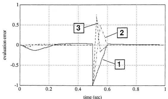
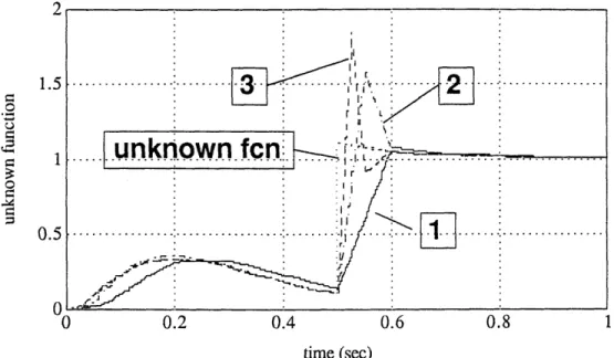
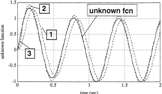
2, 3 shows the simulation curve using Eqn( 2.24), ( 3.8) and ( 3.11) respectively by a same window size L. From the results, we can see that while choosing a larger window to reduce the noise, we can use a more accurate evaluation of the unknown function to improve the performance. Although at the same time, because of the weighting in extrapolating calculation, the noise can be amplified, the scale of this amplification is much smaller than if we choose a small L to achieve the same performance. Fig( 3.7) shows the control actions with noise in each case.
1
0 .5
..
...
...
... ...
....
-0r - L:I-*• II t II -1 0 0.2 0.4 0.6 0.8 1 time (sec)0.2 0.4 0.6 0.8 time (sec)
Figure 3.2: Case I: The evaluated unknown functions.
0.5 1 1.5
time (sec)
Figure 3.3: Case II: The evaluation errors of unknown function.
0.5 I II "¢e
...
unknow.n.fcn..
...
- i ·IrIi...
..
...
.
... :... •I
7 "
.•
..
...
'...
,i' . t-L._. o• 0.6 0.4 0.2 0 -0.2 -0.4 -0 .06 'r o r "- ... c . .... ... 1 -·- ... °ANALYSIS OF ACCURACY
0 0.5 1 1.5
time (sec)
Figure 3.4: Case II: The evaluated unknown functions.
x10-3
0.5 1 1.5 2
time (sec)
Figure 3.5: Case II: The tracking error of xl.
0.5 0 -0.5 -1 -4 0 ~---CHAPTER 3.
0.5 1 1.5 time (sec)
Figure 3.6: Case II: The tracking error of x2.
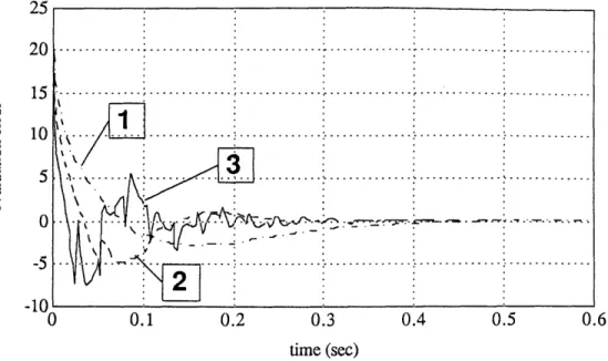
(b)
-- :: 1 0.5 0 -0.5 2 1)
0.5 1 1.5 time (sec) 0 0.5 1 1.5 2 time (sec)(c)
0.5 1 1.5 time (sec) 0 0.5 1 1.5 2 time (sec)(d)
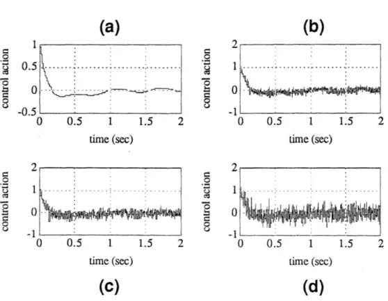
Figure 3.7: Case II: The control actions with 3% noise at the feedback signal. (a) no noise. (b) control action using 4. (c) control action using 4
order2. (d) control action using l4 order3. 0.03 0.02 0.01 -0.01 -0.02 -_n n 0
(a)
~~L~glC~U~I~~~n~LJ k(NW 1 111~IJf ~ I. . . ...
I
Chapter 4
The Stability Conditions
4.1
Stability Conditions for TDC Based on
Con-volutions
In this chapter, a method similar to reference [27] is used to discuss the stability conditions. First it is necessary to state that the values of B, F, D, H has negligible variation within the window if L is chosen small enough. This is justified by Lemma 1 in [27]:
Lemma 1: If the system under consideration and its controller are well defined by Eqn( 2.1) and ( 2.19), ( 2.22) over the interval 0 < t < T, Then B(x), F(x,t), D(t), H(x, t) are uniformly continuous functions of time for 0 < t < T.
Then the following Lemma results.
Lemma 2: Consider the system described in section 2, under the digital form of Time Delay Control with the control action as Eqn( 2.19) and Eqn( 2.24). If
(i) The sampling period is very small : t --+ 0
(ii) B, F, H, D in Eqn( 2.1) have small deviation within the window L
(iii) The digital system z(k) = [(I - B(x)B+ ) C - '][Z = eA(fl-n)ts k-(q-n))] is expo-nentially stable. (where C-1 [=0 eAe(q-n)t ]
-1, and q is the number of data points
within the window L.)
then e(k) = (Am + BK)e(k) can be achieved as time goes on, i.e. k -+ co
Recalling the form in section 2.4, the simplification form of Eqn( 2.22) is
J
o 4(t, r)4'(r)dr= x(t) - # (t, to)x(to)
+j
(t, 7)(A,m + BK)x(r)d---
( (t, ,r)Bu()dT
S(t,
T)F(r)dr
toIf a digital controller is used and let L = qts, the evaluation of unknown function
becomes
q-1 q-1
[(t) e
[ eAe(q-n)tt,]-l[x(t) - eAAeqtjx(t - qt,) + E eA.(q-n)t'sAx(t -
(q
- n)ts)t,n=O n=O
q--1 q-1
--
C
Ae((q-)t"F(t - (q - n)ts)ts ->1
eA(q-n)t"Bu(t - (q - n)ts)ts]n=O n=O
where the first two of the terms between the big brackets can be written as
(4.2)
x(t) - eAe~qtx(t - qts)
x(t) - eAetjx(t
-t
) + eAet"x(t - it
8
,)
-... + eA,(q-1)t"x(t - qt.) - eAeqtsx(t - qt,)When t, - O0, eAet" r, I + Aets, and x(-x(t-) (t - ts), the above equation
becomes
q-1
SeAe(q-n+l)t5x(t
- (q - n)t3)t, - E eA,(q-n)t'Aex(t - (q - n)ts)t,n=O n=O (4.4)
Let [=Io eAe(q-n)ti -1 C-, then
q-1 A (t) a C-1[ eAe(q-n)t5x(t - (q - n)t3) - eAe(q-n)t'F(t - (q - n)t, ) n=O (4.5) n= o q-1
-
•
e(q-n)'tBu(t -
(q
-
n)ts)]
n=OFrom Eqn( 2.14) and Eqn( 2.17) the control action is
u = B+[Ax + Bmr - F(x, t) - W(x, u, t)] - K(xm - x)
(4.1)
(4.3)
q-1
THE STABILITY CONDITIONS From Eqn( 2.1)
5 = F(x, t)+ H(x, t)+ D(t)
+B(x)Bt+[Amx + Bmr - F(x, t) - ,(x, u, t)] - BK(xm - x) Substitute Eqn( 4.5) into the above equation
x = F(x, t) + H(x, t) + D(t) + B(x)B+[Amx + Bmr - F(x, t)
q-1
(4.7)
q- 1
- C-1[ eAe(q-n)t"X(C - (q - ni)t8) - eAe(q-n)u - (q - n)t,)
n=O n=O
q-1
- q eAe(q-"n)'F(t - (q - n)t,)]] - BK(x,. - x) (4.8)
n=O
Since u = B+(k - F - H - D), when B,F,H,D has small deviation within the window with size L, and if the digital form of x(t) is expressed as X(k) (t = kts), the following equation is obtained
q-1
B(x)B+[AmX(k) + Bmr(k) - C-1- Ae(-)t*(I- BB(x)+)±(k_(q-n,)]
n=o -BK(Xm(k) - X(k))
Consider the equation at step k - 1,
- B(x)B•[AmX(k-1) + Bmr(k-1)
q-1
-
C-
1 A(q-n)t,(I_
- B(X)+)x(k-(q-n-1))ts]n=O
-BK(Xm(k-1_l) - X(k-1)) (
Subtract these two equations and let y(i) = x(i) - X(i-1), since when t, -+ 0, X(k-1) -* X(k), Xm(k-1) -+ Xm(k), r(k-1) r(k), the result
is
q-1
Y(k) = B(x)B+[-C-'E eAe(q-n)t( (I- tB(x)+)y(k-(q-n))] (4.11)
n=O
let z = (I - BB(x)+)y
q-1 z(k) =[(I
-B(x)B
+)C
- '][
eAP(q-n)tsz(k-(qn))] n=O (4.12) X(k) X(k-1) (4.9) 4.10) CHAPTER 4.If only the above system is stable, that is, z(k) -+ 0, and thus xc(k-1) -+ (k). closed loop system becomes
B(x)B3+*(k) = B(x)B+[AmX(k)+ Bmr(k)] - BK(Xm(k) - X(k))
The
(4.13) Multiply BB(x)+ to both sides and subtract Eqn( 2.4) from the above equation, we
have
e(k) = (Am + BK)e(k)
(4.14)
This completes the proof.
4.2
Stability Conditions for TDC with
Extrapo-lations
Following the same procedure, we can derive the stability conditions for the control laws which use extrapolations to evaluate the unknown function. The conditions are similar, except that condition (iii) is revised as
. The digital system
Z(k) = [(I - B(x)B+ ) 2_ ][ 2C1E eAe(q-n)tz(k_(qn)) 2 n=0O (4.15) q-1 -C-1 n=O is exponentially stable.
The digital system
Z(k) = [(I - B(x)B~+ ) _-1 4 n=O eA•(q-n),t, Z(k-(q-n)) I-1 2C 7 n=0 eAe(q-n)ts (k-_(q-_n))]
CHAPTER 4. THE STABILITY CONDITIONS 1 q-1
+C-1C
eA(q-)t, (k-(q-n))
(4.16)
n=O is exponentially stable. 2- eA"(o - •) ]- 1 and C, r 4 A, - ,n)t, respectively, where C1 = [=0 Ae()1 and C =eA(-)t - 12 4
4.3
SISO systems
4.3.1
Stabilizing Control Input Gain for TDC Based on
Convolutions
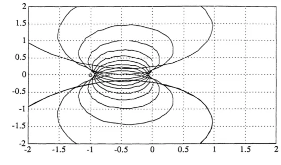
When the system under considerations is a SISO system, a range for b(x)b- 1 can be obtained. By Nyquist stability criteria, using the procedure described in [27], let
[1 - b(x)b-']C-1 = r, and examining the polar plot of the transfer function,
q-1 eA e(q-n)te n
G(z) = zn= q (4.17)
a range -1 _< y < C- 1 is found for system to be stable. Fig( 4.1) and Fig( 4.2) show
the Nyquist plots of G(z) at the two limits when q = 12.
4.3.2
Stabilizing Control Input Gain for TDC with
Extrap-olations
For the control laws which use extrapolations, the range is about -C - 1 < y < aC- 1 where a is a real number between 2 and 3. The value of a depends on q and can be obtained by Nyquist plots for each q. It is clear that the range of stable - 1' is reduced in the latter cases.
4.4
MIMO systems
4.4.1
Issues in MIMO Systems
For MIMO systems, the choice of the matrix B that guarantees stability and accept-able performance can be difficult. Once we have B3, the stability of the system can
be obtained by examining the equation in Lemma 2, condition (iii). q-1
Z(k) = [(I - B(x)I+)C-1][ eAe(q-~n)tz(k-(q-n))]
(4.18)
n=0
However, the choice of the elements in the matrix B is not straightfoward. One way to do it is to find a stabilizing range of III- B(x)jll, where I - I1 represents the norm. This leads to a more conservative result since a norm doesn't include the information about the directions in matrices. Another issue is that different norms lead to different choices of B. It is not clear that which definition of norm gives a better result.
4.4.2
Stabilizing Control Input Gain Matrix for TDC Based
on Convolutions
Using norms, a range corresponding to a stable system is dictated by III - B(x)BII. First, let (I - B(x)tB+) = (. The stability condition Eqn ( 4.18) becomes
Z(k) =- •-1[eAets z(k-1) + eAe2t Z(k-2) + ... + e6etsZ(.(k-q)] (4.19)
Taking the norms, Eqn ( 4.19) becomes
IIZ(k)
II
III
Ic-'
[eA
[ll
st
llIZ(k-.)
+
lj
llZ(k-2)11+
* Aeq (k- q)III
<
I(jIIIC-l
l[IeA)ets
I
lZet(k_-1)H+
lee
t 11 IIZ(k-2)11+
... +lAets
lq IIZ(k-q) II Let IleAetsl = a, jC-111 =f
and 'W(k) =llz(k)jl,
the above equation becomesW(k) -< III 3[aW(k-1) +
z2
W(k_2) + ... + Ctw(k-q)](4.20)
Since W(k) = IIZ(k)II 2 0, it is obvious that if the system described by Eqn ( 4.21) is
stable, then Eqn ( 4.20) is guaranteed to be stable.
CHAPTER 4. THE STABILITY CONDITIONS
Thus, the stability of Eqn ( 4.21) implies the stability of Eqn ( 4.18), since tw(k) -* 0 as k --+ oo implies z(k) -+ 0 as k -- oo1. By the above derivation, the MIMO stability condition is reduced to a scalar system, although this is a conservative sufficient condition. The stabilizing range of 11(11/3 was obtained in the previous section for SISO systems. Therefore, the stabilizing range is found to be III - B(x)B3l| < 1.
4.4.3
Stabilizing Control Input Gain matrix for TDC with
Extrapolations
For the control laws which use extrapolations, the range can be found by the same procedure. However, using this method, the stabilizing range is found to be the same as the cases without using extrapolations. This is because this conservative sufficient condition does not distinguish the signs of the value [I- B(x)B3], and only the positive part of the range is considered.
-1.5 -1 -0.5 0 0.5 1 1.5 2
Figure 4.1: The ploar plot for q = -1.
-0.8 -0.6 -0.4 -0.2 0 0.2 0.4
Figure 4.2: The ploar plot for r = C- 1
1.5 1 0.5 0 -0.5 -1 -1.5 _--2 fl, 0 -1 ,'t
Chapter 5
Frequency Domain Interpretation
5.1
Gain Amplification at Low Frequency
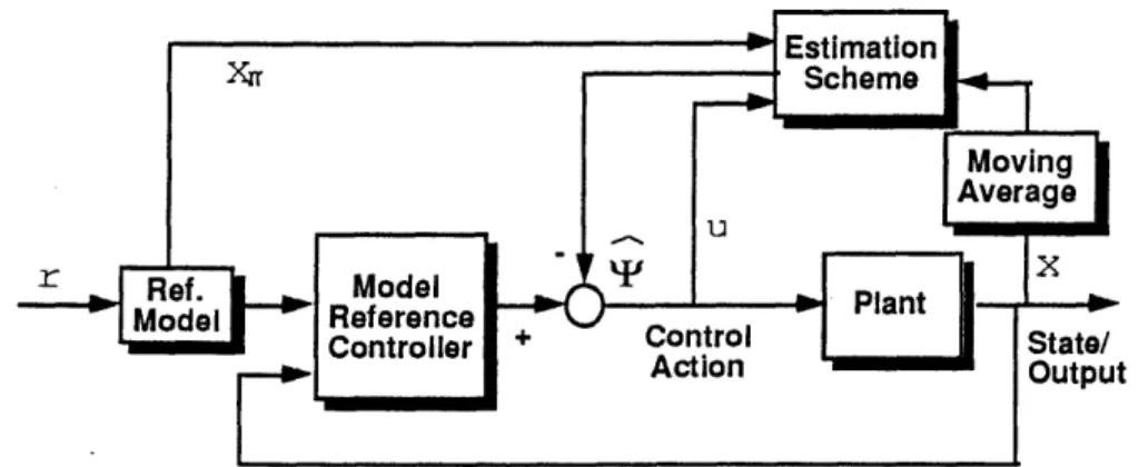
From Eqn( 2.41), it is found that the estimation through digital convolutions is sim-ilar to a "Moving Average" algorithm, which is a well-known form of digital filters. However, as shown in Figure 5.1, the signals go through the moving average block include not only the feedback signals, but also the past control actions. If a linear TDC controller is considered as a special case ( the case when the possibly nonlin-ear function F(x) doesn't appnonlin-ear in the control action), the whole controller fits the "Auto Regressive Moving Average Model" [9]. In this case one can examine the con-troller frequency response. Note that the extrapolation schemes fit the same model with different weighting coefficients. Comparing the frequency responses of the con-trollers using Eqn( 2.24), ( 3.8) and ( 3.11), it was found that the low frequency gains are further increased by the higher order extrapolations while the high frequency re-sponse still rolls off due to the filter effects. This also gives another interpretation for the extrapolation methods that improve the command following and disturbance rejection performances while not significantly amplifying the high frequency noise.
5.2
The Effect of Digital Filter on Stability
Note that in TDC based on convolutions, the weighting coefficients are decided by the convolutions , and they are constants if B is chosen as a constant matrix. If the case
then it might be possible to choose a set of weighting coefficients to reach a better filter effects in comparison to the previously mentioned controllers. Unfortunately, the system will be unstable by doing this in most of the case even when B(x) is exactly known. The reason is that the moving average algorithm introduces extra dynamics which are not counted as part of the plant. Since the relative degree is very important when designing a Time Delay Controller [26], the system is very likely to be unstable. Thus we conclude that using convolutions is a better way of introducing the filter effects while keeping the system stable with a suitably chosen 3.
CHAPTER 5. FREQUENCY DOMAIN INTERPRETATION
Figure 5.1: Time Delay Control schematic with moving average
Figure 5.2: Time Delay Control schematic with moving average only on feedback signals
An MIMO Example
A robot manipulator as Fig( 6.1) was chosen as an example to show the effectiveness of the controllers. This system can be described by the following equations[19],
unit length and unit mass
Figure 6.1: Two degree of freedom robot manipulator
01 02 021
02
1 2(+
cos 02) H = 33 s 2 2 cos 02.
T2
motor 2 +[
where 0 H-1 01 02 l:1 71 (6.1) 3+
cos 02 2 3(6.2)
CHAPTER 6. AN MIMO EXAMPLE
h= 1 H-
[
-02(201+
2) sin 02 2[
01 sin 02The reference model is chosen as (1 = 1, 2 = 1 and Cn1 = 5 and unit step reference input for both links. The delay sampling period is 0.0025 sec. B is chosen as
0
0
0 0 0.75 -0.75-0.75
3.75
(6.3)
rad/sec, W,2 = 6 rad/sectime is 0.1 sec, and the
(6.4)
for simulation case I and
0
0
A
6.3750
0-15.3750
0(6.5)
-15.3750
40.8750
for simulation case II. Fig( 6.2) to Fig( 6.9) shows the results. Line 1, 2, 3 correspond to the simulation curves using 'Y, 1Jor.der2 and 'order3 respectively with the same
window size 0.1sec. Simulation results of case I show that an appropriately chosen B matrix can lead to a good tracking performance, while the extrapolation scheme is used. When the B matrix is poorly chosen as case II, the extrapolation scheme sometimes makes the system go unstable. Fig( 6.10) to Fig( 6.13) show the control actions of link 1 and link 2 when noise is added to the feedback signal. From the above, we can see that a trade-off exists among the noise effect, performance, and robustness.
A I f) V.U3 0.02 0.01
0
-0.01 -0.02 0 error 0.5 1 1.5 2 time (sec)Figure 6.2: Case I: The tracking error of linkl.
error
0.5 1 1.5
time (sec)
Figure 6.3: Case I: The tracking error of link2. 0.0U 0.01 -0.01 -0.02 -0.03 0
CHAPTER 6. AN MIMO EXAMPLE
.6
Figure 6.4: Case I: The
0.2 0.4
time (sec)
evaluation errors of unknown function.
0.6 0.8
time (sec)
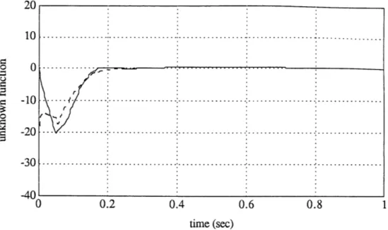
Figure 6.5: Case I: The real (- -) and evaluated (-) unknown functions by '.
20 10 0 -10 -20 -30 -40 C - --- --- --- - ---. . . .. . . ... ... . .... . M 7 = .... -- --- - .. .. --- 7---r
0 -10 -20 -30 -40 -0 0.2 0.4 0.6 0.8 1 time (sec)
Figure 6.6: Case I: The real (- -) and evaluated (-) unknown functions by "1order2*
-40
0 0.2 0.4 0.6 0.8
time (sec)
error U.Z 0.15 0.1 0.05 0 -0.05 -0.1 -0.15 -0.2 error - -- - -I 0.4 0.3 0.2 0.1 0 -0.1 -0.2 -0.3 -0.4 0.5
CHAPTER 6. AN MIMO EXAMPLE
time (sec)
Figure 6.9: Case II: The tracking error of link2.
r---. ,~ ---~- - -- -. -- -- ---. .... ... --- - .--- -- .--- ---0.5 1 1.5 time (sec)
Figure 6.8: Case II: The tracking error of linkl. 0
0 0.2 0.4 0.6 0.8 1 1.2 1.4 1.6 1.8 100 50 0 -50 40 20 0 -20 0 0.2 0.4 0.6 0.8 1 1.2 1.4 1.6 1.8 time (sec)
Figure 6.10: Case I: The control action by IF
0.2 0.4 0.6 0.8 1 12 14 1 6 1i time (sec)
L
. i
.
...
...
...
.... ......
. . . .--20 0 0.2 0.4 0.6 0.8 1 1.2 1.4 1.6 1.8 2 time (sec)Figure 6.11: Case I: The control action by xl with 3% noise at feedback signal. time (sec)
1
...
..
..
.
...
. .
...
...
.
100 50 0.
..
.
.
.
.
..
.
..
.
.
.
.
.
.
.
.
.
.
.
.
...
.
. . .
...
.
...
~.v 1., ... ... v 0 P%... ~~lrlYFNh~l~?~t~dl~YYI* ~ullAN MIMO EXAMPLE
0.2 0.4 0.6 0.8 1 1.2 1.4 1.6 1.8 2 time (sec)
0.2 0.4 0.6 0.8 1 1.2 1.4 1.6 1.8 2 time (sec)
Figure 6.12: Case I: The control action by 1
'order2 with 3% noise at feedback signal.
0 0.2 0.4 0.6 0.8 1 1.2 1.4 1.6 1.8
time (sec)
•- - -
-0 0.2 0.4 0.6 0.8 1 1.2 1.4 1.6 1.8 2
time (sec)
Figure 6.13: Case I: The control action by xiorder3 with 3% noise at feedback signal.
0 100 50 0 -50 -20 0
... ... --- ... ... ... ...
!:Jti~~~lp.Ih~c~~~* .~i SF rly~i~-J rhiiL;~
200 100 0 100 40 20 0 -20 I _· --- - -- - : : : : :
h
...
..
...
...
...
..
.2
...
... ... ... ... ... . CHAPTER 6. I (-
i
i
,,
Application to a Cruise Control System
In this chapter, an application of Time Delay Control to an intelligent automotive cruise control system is presented to show the performance of Time Delay Control on actual systems. In this system, a vehicle is equipped with a ranging sensor which mea-sures the distance between a preceding car and itself. The relative distance between the two vehicles is the control output [the state] of the system and the dynamics of the leading car are treated as a disturbance. The performance of the Time Delay Con-trol Method in this intelligent longitudinal cruise conCon-trol system was evaluated using a one-fifth scale car model. Through simulations and experiments, the Time Delay Control technique is shown to be well suited for intelligent cruise controls because of its rapid estimation of system dynamics changes and ease of implementation.7.1
Introduction to an Intelligent Cruise Control
System
There are several aspects to intelligent vehicle systems. For example, engine control, anti-skid braking and active suspension systems have been developed to try to auto-matically optimize fuel consumption, prevent wheel locking and minimize vehicle roll based on control algorithms. The driver and passengers benefits from these systems include savings, safety, and comfort.
An intelligent cruise control system may be capable of maintaining a constant speed or constant distance from a primary vehicle' (longitudinal control) as well as
1
CHAPTER 7. APPLICATION TO A CRUISE CONTROL SYSTEM
directing lateral motions of the vehicle. This paper focuses on the use of Time Delay Control for longitudinal control and demonstration of its advantages. Attempting longitudinal control requires that the algorithm guarantees acceptable error dynamics (disturbance rejection) for large, unexpected disturbances. Such disturbances may be acceleration or deceleration of the primary car, changes in road conditions, changes in grade, and changes in wind. All of these disturbances will cause an error in the distance between the primary and secondary vehicles. Unless the error dynamics of the controller are guaranteed, collision avoidance could be imminent.
The control strategy considered consists of at least two levels: a high level con-troller and a low level concon-troller. The high level concon-troller may perform several func-tions :(1) observes the state of the system,(2) accepts inputs from environment,(3) performs filtering and estimation, (4) decides whether a task is realizable, etc.... It then generates commands which are sent to a low level controller. The low level controller on the other hand has a few other functions: (1) observes the state of the system, (2) filters and estimates and (3) computes the control action. The control action is generated in order to execute realizable commands issued by the high level controller independent of system dynamic variations. These variations may be due to internal system changes or external disturbances. Internal factors may include parameter changes and/or function changes. We are interested in designing low level controllers that guarantee the proper execution of realizable tasks.
7.2
Introduction to the System under
Consider-ation
A one-fifth scale car model shown in Figure 7.1 is used to perform the experiment. The car model is assumed to posses a ranging sensor which could measure the distance paper, is defined as the car intended to follow the preceding one.
between a preceding car and itself. A chassis roller was used to produce unexpected disturbances such as changes in slopes of road and inertia of the vehicle.
The system is considered as
=C=d
dx=
d =
]
I
+
b
u
(7.1)
where d is the longitudinal relative distance (the distance between the primary car and the secondary car), rI, is defined by Equation ( 2.7) and includes the unknown dynamics of the secondary vehicle and disturbance introduced by the primary vehicle. The reference model is defined as
1m dml+ r (7.2)
S dmJ -- aml -am 2 m bm (7.2)
The tracking error e between the desired relative distance trajectory dm and the actual desired relative distance d, and the feedback gain matrix K are given by
e = = dm - d K= k iT (7.3)
e
dm - d
k2
7.3
Controller Design
The TDC has some unique characteristics which are specially advantageous in this cruise control system. The experiments presented in this section are intended to show these effects. One of them is the tracking of a reference model which guar-antee smooth acceleration and desired velocity, and position curves. The controller guarantees system robustness without detailed knowledge of the system dynamics. Consequently, the controller is easy to design and implement. Moreover, the effect of fast disturbance rejection enables the controller to use the relative distance as a feedback signal, observing the changing position of the primary vehicle as a distur-bance, and reject it in several sampling periods. This can be achieved by using the