Algorithms for Persistent Autonomy and
Surveillance
by
Cenk Baykal
Submitted to the Department of Electrical Engineering and Computer
Science
in partial fulfillment of the requirements for the degree of
Master of Science in Electrical Engineering and Computer Science
at the
MASSACHUSETTS INSTITUTE OF TECHNOLOGY
June 2017
c
○ Massachusetts Institute of Technology 2017. All rights reserved.
Author . . . .
Department of Electrical Engineering and Computer Science
May 18, 2017
Certified by . . . .
Daniela Rus
Professor of Electrical Engineering and Computer Science
Thesis Supervisor
Accepted by . . . .
Leslie A. Kolodziejski
Professor of Electrical Engineering and Computer Science
Chair, Department Committee on Graduate Theses
Algorithms for Persistent Autonomy and Surveillance
by
Cenk Baykal
Submitted to the Department of Electrical Engineering and Computer Science on May 18, 2017, in partial fulfillment of the
requirements for the degree of
Master of Science in Electrical Engineering and Computer Science
Abstract
In this thesis, we consider the problem of monitoring stochastic, time-varying events occurring at discrete locations. Our problem formulation extends prior work in per-sistent surveillance by considering the objective of successfully completing monitor-ing tasks in unknown, dynamic environments where the rates of events are time-inhomogeneous and may be subject to abrupt changes. We propose novel monitoring algorithms that effectively strike a balance between exploration and exploitation as well as a balance between remembering and discarding information to handle tempo-ral variations in unknown environments. We present analysis proving the favorable properties of the policies generated by our algorithms and present simulation results demonstrating their effectiveness in several monitoring scenarios inspired by real-world applications. Our theoretical and empirical results support the applicability of our algorithm to a wide range of monitoring applications, such as detection and tracking efforts at a large scale.
Thesis Supervisor: Daniela Rus
Acknowledgments
I am grateful for the people who have encouraged and supported me throughout my research and my first years in graduate school. First and foremost, I would like to thank my advisor, Daniela Rus, for all her invaluable guidance and encouragement. Daniela has been an enthusiastic and remarkable advisor who has used every oppor-tunity to teach me how to be a better researcher and help me grow as a person.
I would also like to thank my collaborators Guy Rosman, Sebastian Claici, Mark Donahue, and Kyle Kotowick for fruitful discussions and their invaluable contribu-tions, without which this thesis would not have been possible. They have generously provided their time and expertise during inspiring discussions that culminated in many of the ideas in this thesis.
Most importantly, I would like to thank my friends and family for their uncondi-tional support and understanding.
Contents
1 Introduction 13 1.1 Contributions . . . 14 1.2 Outline of Thesis . . . 15 2 Related Work 17 2.1 Persistent Surveillance . . . 172.2 Mobile Sensor Scheduling and Coverage . . . 18
2.3 Multi-armed Bandits . . . 19
3 Unknown, Static Environments 23 3.1 Problem Definition . . . 23
3.2 Methods . . . 25
3.2.1 Algorithm for Monitoring Under Unknown Event Rates . . . . 25
3.2.2 Learning and Approximating Event Statistics . . . 27
3.2.3 Per-cycle Optimization and the Uncertainty Constraint . . . . 27
3.2.4 Controlling Approximation Uncertainty . . . 28
3.2.5 Generating Balanced Policies that Consider Approximation Un-certainty . . . 30
3.3 Analysis . . . 31
3.4 Results . . . 35
3.4.1 Synthetic Scenario . . . 37
4 Unknown, Dynamic Environments 41
4.1 Problem Definition . . . 41
4.2 Methods . . . 43
4.3 Analysis . . . 45
4.3.1 Preliminaries . . . 45
4.3.2 Regret over an epoch . . . 48
4.3.3 Total Regret . . . 54
4.4 Results . . . 55
4.4.1 Sinusoidal Variations . . . 56
4.4.2 Discrete Random Walk . . . 56
5 Conclusion 61 5.1 Conclusion . . . 61
5.2 Limitations and Future Work . . . 62
A Technical Supplement to the Theoretical Results in Chapter 3 63 A.1 Proof of Lemma 2 . . . 63
A.2 Proof of Lemma 3 . . . 64
A.3 Proof of Theorem 2 . . . 65
List of Figures
1-1 An example application of a monitoring procedure where a UAV is tasked with monitoring urban events. The colored nodes denote the discrete, spatially-distributed landmarks where pertinent events occur. The monitoring objective is to optimize the monitoring objectives, e.g., maximize the number of event sightings, in an efficient manner [38]. . 14
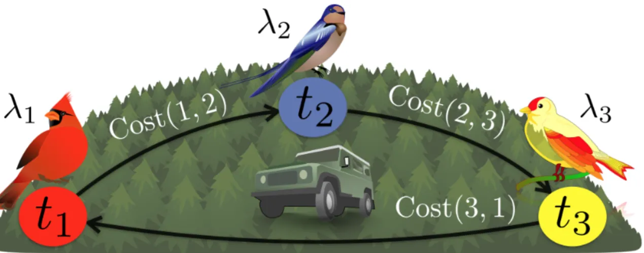
3-1 An example surveillance setting where the objective is to monitor three different species of birds that appear in discrete, species-specific loca-tions. The overarching objective is to observe as many bird sightings as possible in a balanced way, so that an approximately uniform amount of data is collected across all bird species. . . 24
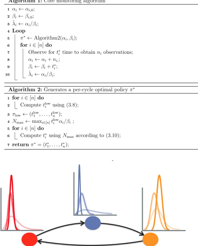
3-2 A depiction of the resulting distributions over event rates at each loca-tion over multiple cycles (faded colors) when the uncertainty constraint is incorporated into the optimization. The uncertainty constraint en-ables the uncertainty at each location to decay in a controlled and uniform way over multiple cycles. . . 26
3-3 The water-filling algorithm described by Sec. 3.2.5 where the colors denote three different discrete locations. The observation times for sta-tions below the bottle-neck expected number of events (dashed black line) is increased until the (approximate) expected number of observa-tions at each station is equivalent. . . 30
3-4 A unified visualization of the components of our algorithm. The lower bounds for the observation times are generated according to the un-certainty constraint in order to ensure controlled decay of unun-certainty (Left). The lower bounds are then utilized by the water-filling algo-rithm detailed in Sec. 3.2.5 to generate policies that are balanced. The conjunction of these two components culminates in monitoring policies that are conducive to both exploration and exploitation. . . 31
3-5 Results of the synthetic simulation averaged over 10,000 trials that characterize and compare our algorithm to the four monitoring algo-rithms in randomized environments containing three discrete stations. 36
3-6 Viewpoints from two stations in the ARMA simulation of the yellow backpack scenario. Agents wearing yellow backpacks whose detections are of interest appear in both figures. . . 38
3-7 The performance of each monitoring algorithm evaluated in the ARMA-simulated yellow backpack scenario. . . 39
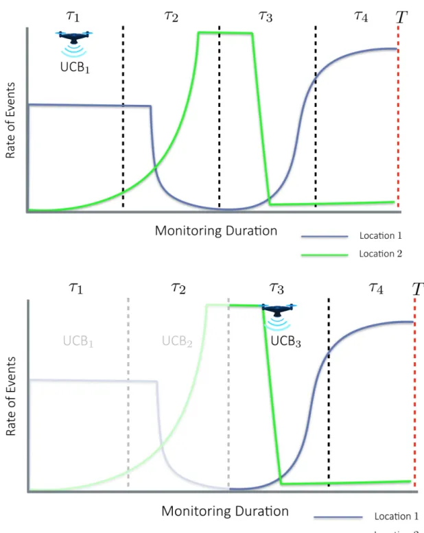
4-1 An example instance of our algorithm, depicting the partitioning of the monitoring period 𝑇 into epochs of length 𝜏 . Within each epoch, the robot executes our variant of the Upper Confidence Bounds (UCB) al-gorithm to balance exploration and exploitation. Information obtained from prior epochs is purposefully discarded at the start of each epoch in order to adapt to the temporal variations in the environment. . . . 44
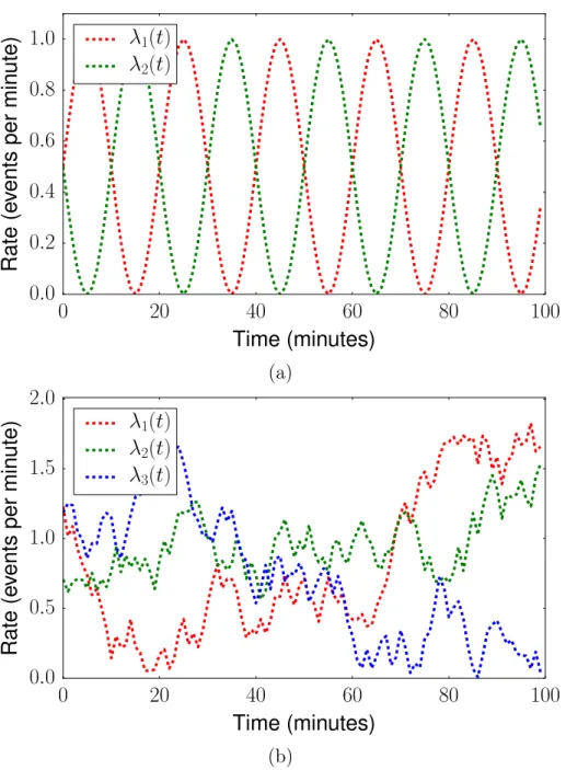
4-2 The two scenarios explored in our experiments. a) The sinusoidal rates of each Poisson process as a function of time with𝑉𝑇 =
√
𝑇 and 𝑇 = 100 minutes. b) The rates of each Poisson process as a function of time generated by a discrete random walk as described in Sec. 4.4.2. The figure depicts the rates of three stations over a time horizon 𝑇 = 100 minutes and variation budget 𝑉𝑇 =𝑇2/3. . . 58
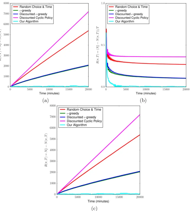
4-3 a) Plot of total regret 𝑅(𝜋, 𝑇 ) = 𝑁*
𝑇 − 𝑁(𝜋, 𝑇 ) over time. The figure
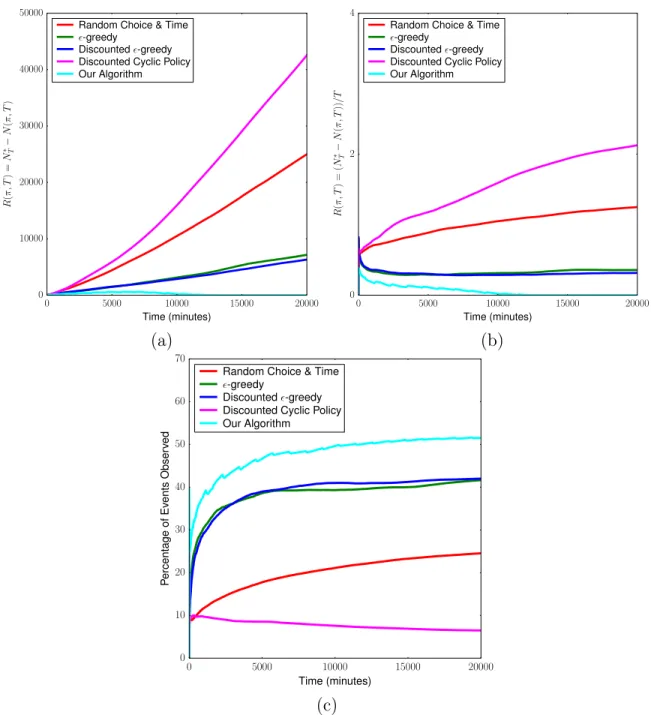
depicts sub-linear growth of regret over time for our algorithm (cyan), as expected from our theoretical results (Sec. 3.3). b) Growth of total regret over time expressed as the quotient 𝑅(𝜋, 𝑇 )/𝑇 . Our algorithm achieves sub-linear regret over time and that 𝑅(𝜋, 𝑇 )/𝑇 → 0. c) Per-centage of events observed with respect to the sum of events that oc-curred across all stations in the environment subject to sinusoidal vari-ation over time. Our algorithm approximately attains optimal number of expected events in this setting consisting of 2 stations. . . 59 4-4 Clockwise a) Total regret as a function of time, i.e. 𝑅(𝜋, 𝑇 ) = 𝑁*
𝑇 −
𝑁 (𝜋, 𝑇 ), in the simulated scenario involving discontinuous, abrupt changes. Our algorithm (shown in cyan) achieves the lowest regret at all times of the allotted monitoring time 𝑇 = 20, 000 minutes. b) Growth of the total regret over time,𝑅(𝜋, 𝑇 )/𝑇 , in an abruptly chang-ing environment. c) Percentage of events observed with respect to all of the events that transpired in the abruptly changing environment (Sec. 4.4.2) at all stations during the time horizon T. . . 60
Chapter 1
Introduction
Persistent surveillance tasks often require the agent to monitor stochastic events of in-terest in unknown, dynamic environments over long periods of time in an autonomous manner. Equipped with limited a priori knowledge, uncertainty over time-varying event statistics necessitates the robot to travel from one landmark to another, identify the regions of importance, and adapt to the temporal variations in the environment. The overarching objective is to maximize the number of events observed in order to enable efficient data collection, which may be imperative for a successful surveillance mission. Applications include monitoring of wildlife, natural phenomena (e.g., floods, volcanic eruptions), urban events (see Fig. 1-1), and friendly and unfriendly activities. In this thesis, we consider a novel persistent surveillance problem in which a mobile robot is tasked with monitoring transient events that occur in discrete, spatially-distributed landmarks according to station-specific Poisson processes with unknown, time-varying statistics. We assume that the monitoring task is conducted by a single robot equipped with a limited-range sensor that can only record measurements when the robot is stationary at a location, i.e., it cannot make measurements while traveling. Hence, the robot must travel to each location and wait for transient events to occur for an appropriately generated amount of time before traveling to another location. The persistent surveillance problem is to generate an optimal sequence of location-time pairs that optimizes the monitoring objectives at hand, e.g., maximizes the number of events observed in a balanced manner across all regions of interest.
Figure 1-1: An example application of a monitoring procedure where a UAV is tasked with monitoring urban events. The colored nodes denote the discrete, spatially-distributed landmarks where pertinent events occur. The monitoring objective is to optimize the monitoring objectives, e.g., maximize the number of event sightings, in an efficient manner [38].
1.1
Contributions
This thesis contributes the following:
1. Persistent surveillance problem formulations that relax the assumptions of (i) known event statistics and (ii) static event statistics, commonly imposed by prior work.
2. A persistent surveillance problem formulation that bridges the monitoring ob-jective of maximizing event observations with the obob-jective of minimizing regret by introducing a new definition of weak regret for persistent surveillance. 3. A novel monitoring algorithm for generating appropriate policies to monitor
transient events in unknown, dynamic environments where the total variation over time is bounded by a variation budget 𝑉𝑇 that is known a priori.
4. An analysis proving that under the assumption that the total variation of the event rates is bounded by a variation budget𝑉𝑇 =𝑜(𝑇 ), our algorithm generates
long-run average optimal policies.
regret (i.e., maximizing the number of event observations) in several dynamic and random environments and comparing its performance to adaptive monitor-ing algorithms.
1.2
Outline of Thesis
The outline of this thesis is as follows. In Chapter 2, we present related work in per-sistent surveillance and discuss the limitations of current state-of-the-art monitoring approaches. In Chapter 3, we present the multi-objective persistent monitoring prob-lem formulation that relaxes the assumption of known event statistics in otherwise static environments. We formulate and analyze a monitoring algorithm capable of balancing exploration and exploitation in the environment when the agent is initially equipped with limited a priori knowledge.
In Chapter 4, we further extend the canonical persistent surveillance problem for-mulation by relaxing the assumption of static event statistics and consider monitoring events in unknown and dynamic environments. We present and analyze a Multi-armed Bandits inspired approach that overcomes the limitations of prior approaches by generating policies in consideration of temporal variations and the exploration and exploitation trade-off. We conclude with a discussion of the presented approaches and their limitations, and provide suggestions for avenues of future research in Chapter 5,
Chapter 2
Related Work
Our work leverages and builds upon prior work in persistent surveillance, mobile sensor scheduling, and stochastic optimization.
2.1
Persistent Surveillance
The problem of persistent surveillance has been studied in a variety of real-world in-spired monitoring applications such as underwater marine monitoring and detection of natural phenomena [6,11,21,22,25,26,30,32–34,36]. These approaches generally as-sume that the robot can obtain measurements while moving and generate paths that optimize an application-specific monitoring objective, such as mutual information. Further examples of monitoring objectives include facilitating high-value data collec-tion for autonomous underwater vehicles [32], keeping a growing spatio-temporal field bounded using speed controllers [34], and generating the shortest watchman routes along which every point in a given space is visible [12].
Other related work in persistent surveillance includes variants and applications of the Orienteering Problem (OP) to generate informative paths that are constrained to a fixed length or time budget [18]. Yu et al. present an extension of OP to monitor spatially-correlated locations within a predetermined time [40]. In [15] and [39] the authors consider the OP problem in which the reward accumulated is characterized by a known function of the time spent at each point of interest. In contrast to
our work, approaches in OP predominantly consider known, static environments and budget-constrained policies that visit each location at most once.
Surveillance of discrete landmarks is of particular relevance to our work. Monitor-ing discrete locations such as buildMonitor-ings, windows, doors usMonitor-ing a team of autonomous micro-aerial vehicles (MAVs) is considered in [26]. [1] presents different approaches to the min-max latency walk problem in a discrete setting. [38] extends this work to include multiple objectives, i.e. [38] considers the objective of minimizing the maxi-mum latency and maximizing balance of events across stations using a single mobile robot. The authors show a reduction of the optimization problem to a quasi-convex problem and prove that a globally optimal solution can be computed in 𝑂(poly(𝑛)) time where𝑛 is the number of discrete landmarks. Persistent surveillance in a discrete setting can be extended to the case of reasoning over different trajectories as shown in [30, 34, 35]. However, most prior work assumes that the rates of events are known prior to the surveillance mission, which is very often not the case in real world robotics applications. In this thesis, we relax the assumption of known rates and present an algorithm with provable guarantees to generate policies conducive to learning event rates and optimizing the monitoring objectives.
2.2
Mobile Sensor Scheduling and Coverage
The problem of persistent surveillance can be formulated as a mobile sensor schedul-ing problem and has been studied extensively in this context [16,19,20,27]. Persistent surveillance is closely related to sensor scheduling [19], sensor positioning [20], and coverage [16]. Previous approaches have considered persistent monitoring in the con-text of a mobile sensor [27].
Mobile sensor scheduling in environments with discrete landmarks are of particular relevance to our work. For instance, [26] considers monitoring discrete locations such as buildings, windows, and doors using a team of autonomous micro-aerial vehicles (MAVs). In [1], the authors present an approach to the min-max latency walk problem and [38] extends this work to the multi-objective mobile sensor scheduling problem for
surveillance of transient events occurring in discrete locations in the environment with known event rates and proposes an algorithm for generating the unique optimal policy maximizing the balance of observations while minimizing latency of observations at each station.
Yu et al. present an extension of OP to monitor spatially-correlated locations within a predetermined time [40]. In [15] and [39] the authors consider the OP problem in which the reward is a known function of the time spent at each point of interest. In contrast to our work, approaches in OP predominantly consider known environments and budget-constrained policies that visit each location at most once and optimize only a single objective.
[11] considers controlling multiple agents to minimize an uncertainty metric in the context of a 1D spatial domain. Decentralized approaches to controlling a network of robots for purposes of sensory coverage are investigated in [30], where a control law to drive a network of mobile robots to an optimal sensing configuration is pre-sented. Persistent monitoring of dynamic environments has studied in [25,33,34]. For instance, [25] considers optimal sensing in a time-changing Gaussian Random Field and proposes a new randomized path planning algorithm to find the optimal infinite horizon trajectory. [10] presents a surveillance method based on Partially Observable Markov Decision Processes (POMDPs), however, POMDP-based approaches are of-ten computationally intractable, especially when the action set includes continuous parameters, as in our case.
2.3
Multi-armed Bandits
As exemplified by the aforementioned works, a variety of monitoring algorithms have been presented and shown to perform well empirically. However, literature on meth-ods with theoretical performance guarantees in unknown, time-varying environments has been sparse and limited. The added complexity stems from the inherent explo-ration and exploitation trade-off, which has been rigorously addressed and analyzed in Reinforcement Learning [23, 24, 28] and the Multi-armed Bandit (MAB)
litera-ture [3,4,9]. However, the traditional MAB problem considers minimizing regret with respect to the accumulated reward by appropriately pulling one of the𝐾 ∈ N+ levers
at each discrete time step to obtain a stochastic reward that is generally assumed to bounded or subgaussian. Our work differs from the traditional MAB formulation in that we consider optimization in the face of travel costs, non-stationary processes, distributions with infinite support, and continuous state and parameter space. To the best of our knowledge, this thesis presents the first treatment of a MAB variant exhibiting all of the aforementioned complexities and a monitoring algorithm with provable regret guarantees with respect to the number of events observed.
MAB formulations that relax the assumptions of the traditional MAB problem are of particular pertinence to our work. Besbes et al. present a non-stationary MAB formulation where the variation of the rewards are bounded by a variation budget𝑉𝑇
and present policies that achieve a regret of order (𝐾𝑉𝑇)1/3𝑇2/3, which is long-run
average optimal if the variation 𝑉𝑇 is sub-linear with respect to the time horizon
𝑇 [5]. The authors mathematically show the difficulty of this problem by proving the lower bound of Ω((𝐾𝑉𝑇)1/3𝑇2/3), which implies that long-run average optimality is
not achievable whenever 𝑉𝑇 is linear in 𝑇 .
Garivier et al. consider a non-stationary MAB setting where the distributions of the rewards change abruptly at unknown time instants, but the number of changes up to time𝑇 , Υ𝑇, is bounded and known in advance [17]. The authors present discounted
and sliding window variants of the Upper Confidence Bound (UCB) algorithm [3, 4] that achieve a regret of 𝑂(√𝑇 Υ𝑇log𝑇 ) and also prove the lower-bound of Ω(
√ 𝑇 Υ𝑇)
on the achievable regret in this setting, which is linear if the number of abrupt changes grows linearly with time. Prior work on the MAB formulation with switching costs tells a similar story regarding the difficulty of the aforementioned MAB extensions: Dekel et al. prove the lower-bound of ˜Ω(𝑇2/3) on the achievable regret in the presence
of switching costs [14].
Recently, Srivastava et al. presented an approach with a provable upper bound on the number of visits to sub-optimal regions that bridges surveillance and MAB for monitoring phenomena in an unknown, abruptly changing environment [37]. However,
their approach considers a discrete state and parameter space (i.e., the generation of observation times is not considered), assumes Gaussian distributed random variables –which may be less suitable for monitoring instantaneous events (such as arrivals), assumes that the number of abrupt changes are bounded and known in advance, and does not explicitly take travel cost into consideration.
We build upon prior work and consider an unknown, dynamic environment where the robot is tasked with visiting each location more than once, observing stochas-tic, instantaneous events for an appropriately generated time, and adapting to the temporal variations in the environment over an unbounded amount of time. Un-like prior work in persistent surveillance which has focused on environments with a bounded number of abrupt changes, our problem formulation extends to continuously-varying as well as to abruptly-changing environments, as long as the total variation is bounded [5]. We introduce novel monitoring algorithms with provable guaran-tees with respect to the number of event sightings and present simulation results of real-world inspired monitoring scenarios that support our theoretical claims.
Chapter 3
Unknown, Static Environments
We begin by relaxing the assumption of known event statistics and consider the problem of persistent surveillance when the agent is equipped with limited a priori knowledge about the environment.
3.1
Problem Definition
Let there be𝑛∈ N+spatially-distributed stations in the environment whose locations
are known. At each station 𝑖 ∈ [𝑛], stochastic events of interest occur according to a Poisson process with an unknown, station-specific rate parameter 𝜆𝑖 that is
independent of other stations’ rates. We assume that the robot executes a given cyclic path, taking 𝑑𝑖,𝑗 > 0 time to travel from station 𝑖 to station 𝑗 and let 𝐷 :=
∑︀𝑛−1
𝑖=1 𝑑𝑖,𝑖+1+𝑑𝑛,1 denote the total travel time per cycle. The robot can only observe
events at one station at any given time and cannot make observations while traveling. We denote each complete traversal of the cyclic path as a monitoring cycle, indexed by 𝑘 ∈ N+. We denote the observations times for all stations 𝜋𝑘 := (𝑡1,𝑘, . . . , 𝑡𝑛,𝑘)
as the monitoring policy at cycle 𝑘. Our monitoring objective is to generate poli-cies that maximize the number of events observed in a balanced manner across all stations within the allotted monitoring time 𝑇max that is assumed to be unknown
and unbounded. We introduce the function 𝑓obs(Π) that computes the total
Figure 3-1: An example surveillance setting where the objective is to monitor three different species of birds that appear in discrete, species-specific locations. The over-arching objective is to observe as many bird sightings as possible in a balanced way, so that an approximately uniform amount of data is collected across all bird species.
∑︀
𝜋𝑘
∑︀
𝑖∈[𝑛]E[𝑁𝑖(𝜋𝑘)], where 𝑁𝑖(𝜋𝑘) is the Poisson random variable, with
realiza-tion 𝑛𝑖,𝑘, denoting the number of events observed at station 𝑖 under policy 𝜋𝑘 and
E[𝑁𝑖(𝜋𝑘)] := 𝜆𝑖𝑡𝑖,𝑘 by definition.
To reason about balanced attention, we let 𝑓bal(Π) denote as in [38] the expected
observations ratio taken over the sequence of policies Π:
𝑓bal(Π) := min 𝑖∈[𝑛] ∑︀ 𝜋𝑘E[𝑁𝑖(𝜋𝑘)] ∑︀ 𝜋𝑘 ∑︀𝑛 𝑗=1E[𝑁𝑗(𝜋𝑘)] . (3.1)
The idealized persistent surveillance problem is then:
Problem 1 (Idealized Persistent Surveillance Problem). Generate the optimal se-quence of policies Π* = argmaxΠ∈𝑆𝑓obs(Π) where 𝑆 is the set of all possible policies
that can be executed within the allotted monitoring time 𝑇max.
Generating the optimal solution Π* at the beginning of the monitoring process is challenging due to the lack of knowledge regarding both the upper bound 𝑇max and
the station-specific rates. Hence, instead of optimizing the entire sequence of policies at once, we take a greedy approach and opt to subdivide the problem into multiple, per-cycle optimization problems. For each cycle 𝑘 ∈ N+, our goal is to adaptively
generate the policy 𝜋*
most up-to-date knowledge of event statistics. We let ˆ𝑓bal represent the per-cycle counterpart of 𝑓bal ˆ 𝑓bal(𝜋𝑘) := min 𝑖∈[𝑛] E[𝑁𝑖(𝜋𝑘)] ∑︀𝑛 𝑗=1E[𝑁𝑗(𝜋𝑘)] .
We note that the set of policies that optimize ˆ𝑓bal is uncountably infinite and
policies of all possible lengths belong to this set [38]. To generate observation times that are conducive to exploration, we impose the hard constraint 𝑡𝑖,𝑘 ≥ 𝑡low𝑖,𝑘 on each
observation time, where𝑡low
𝑖,𝑘 is a lower bound that is a function of our uncertainty of
the rate parameter 𝜆𝑖 (see Sec. 3.2). The optimization problem that we address in
this thesis is then of the following form:
Problem 2 (Per-cycle Monitoring Optimization Problem). At each cycle 𝑘 ∈ N+,
generate a per-cycle optimal policy 𝜋*
𝑘 satisfying 𝜋𝑘* ∈ argmax 𝜋𝑘 ˆ 𝑓bal(𝜋𝑘) s.t. ∀𝑖 ∈ [𝑛] 𝑡𝑖,𝑘 ≥ 𝑡low𝑖,𝑘. (3.2)
3.2
Methods
In this section, we present our monitoring algorithm and detail the main subrou-tines employed by our method to generate dynamic, adaptive policies and interleave learning and approximating of event statistics with policy execution.
3.2.1
Algorithm for Monitoring Under Unknown Event Rates
The entirety of our persistent surveillance method appears as Alg. 1 and employs Alg. 2 as a subprocedure to generate adaptive, uncertainty-reducing policies for each monitoring cycle.
Algorithm 1: Core monitoring algorithm 1 𝛼𝑖 ← 𝛼𝑖,0; 2 𝛽𝑖 ← 𝛽𝑖,0; 3 ˆ𝜆𝑖 ← 𝛼𝑖/𝛽𝑖; 4 Loop 5 𝜋* ← Algorithm2(𝛼𝑖, 𝛽𝑖); 6 for 𝑖∈ [𝑛] do
7 Observe for 𝑡*𝑖 time to obtain 𝑛𝑖 observations; 8 𝛼𝑖 ← 𝛼𝑖+𝑛𝑖,;
9 𝛽𝑖 ← 𝛽𝑖+𝑡*𝑖; 10 ˆ𝜆𝑖 ← 𝛼𝑖/𝛽𝑖;
Algorithm 2: Generates a per-cycle optimal policy𝜋* 1 for 𝑖∈ [𝑛] do
2 Compute 𝑡low𝑖 using (3.8); 3 𝜋low← (𝑡low1 , . . . , 𝑡low𝑛 );
4 𝑁max← max𝑖∈[𝑛]𝑡low𝑖 𝛼𝑖/𝛽𝑖 ; 5 for 𝑖∈ [𝑛] do
6 Compute 𝑡*𝑖 using 𝑁max according to (3.10); 7 return𝜋* = (𝑡*1, . . . , 𝑡*𝑛);
Figure 3-2: A depiction of the resulting distributions over event rates at each location over multiple cycles (faded colors) when the uncertainty constraint is incorporated into the optimization. The uncertainty constraint enables the uncertainty at each location to decay in a controlled and uniform way over multiple cycles.
3.2.2
Learning and Approximating Event Statistics
We use the Gamma distribution as the conjugate prior for each rate parameter be-cause it provides a closed-form expression for updating the posterior distribution after observing events. We let Gamma(𝛼𝑖, 𝛽𝑖) denote the Gamma distribution with
hyper-parameters 𝛼𝑖, 𝛽𝑖 ∈ R+ that are initialized to user-specified values 𝛼𝑖,0, 𝛽𝑖,0 for all
stations 𝑖 and are updated as new events are observed.
For any arbitrary number of events 𝑛𝑖,𝑘 ∈ N observed in 𝑡𝑖,𝑘 time, the posterior
distribution is given by Gamma(𝛼𝑖+𝑛𝑖,𝑘, 𝛽𝑖 +𝑡𝑖,𝑘) for any arbitrary station 𝑖 ∈ [𝑛]
and cycle 𝑘 ∈ N+. For notational convenience, we let 𝑋𝑖𝑘 := (𝑛𝑖,𝑘, 𝑡𝑖,𝑘) represent
the summary of observations for cycle 𝑘 ∈ N+ and define the aggregated set of
observations up to any arbitrary cycle as 𝑋1:𝑘
𝑖 := {𝑋𝑖1, 𝑋𝑖2, . . . , 𝑋𝑖𝑘} for all stations
𝑖 ∈ [𝑛]. After updating the posterior distribution using the hyper-parameters, i.e. 𝛼𝑖 ← 𝛼𝑖 +𝑛𝑖,𝑘, 𝛽𝑖 ← 𝛽𝑖 +𝑡𝑖,𝑘, we use the maximum probabiliy estimate of the rate
parameter 𝜆𝑖, denoted by ˆ𝜆𝑖,𝑘 for any arbitrary station 𝑖:
ˆ 𝜆𝑖,𝑘 :=𝐸[𝜆𝑖|𝑋𝑖1:𝑘] = 𝛼𝑖,0+∑︀𝑛𝑘=1𝑛𝑖,𝑘 𝛽𝑖,0+ ∑︀𝑛 𝑘=1𝑡𝑖,𝑘 = 𝛼𝑖 𝛽𝑖 . (3.3)
3.2.3
Per-cycle Optimization and the Uncertainty Constraint
Inspired by confidence-based MAB approaches [2–4], our algorithm adaptively com-putes policies by reasoning about the uncertainty of our rate approximations. We introduce the uncertainty-constraint, an optimization constraint that enables the gen-erating a station-specific observation time based on uncertainty of each station’s pa-rameter. The constraint helps bound the policy lengths adaptively over the course of the monitoring process so that approximation uncertainty decreases uniformly across all stations. We use the posterior variance of the rate parameter 𝜆𝑖, Var(𝜆𝑖|𝑋𝑖1:𝑘), as
our uncertainty measure of each station𝑖 after executing 𝑘 cycles. We note that in our Gamma-Poisson model, Var(𝜆𝑖|𝑋𝑖1:𝑘) :=
𝛼𝑖
𝛽2 𝑖
Uncertainty constraint For a given𝛿 ∈ (0, 1), 𝜖 ∈(︀0, 2(1+2𝑒1/𝜋)−1)︀ and arbitrary
cycle𝑘 ∈ N+,𝜋𝑘 must satisfy the following
∀𝑖 ∈ [𝑛] P(︀(︀Var(𝜆𝑖|𝑋𝑖1:𝑘, 𝜋𝑘)≤ 𝛿Var(𝜆𝑖|𝑋𝑖1:𝑘−1)
⃒ ⃒𝑋1:𝑘−1
𝑖 )︀)︀ > 1 − 𝜖. (3.4)
We incorporate the uncertainty constraint as a hard constraint and recast the per-cycle optimization problem from Sec. 3.1 in terms of the optimization constraint. Problem 3 (Recast Per-cycle Monitoring Optimization Problem). For each monitor-ing cycle 𝑘 ∈ N+ generate a per-cycle optimal policy 𝜋𝑘* that simultaneously satisfies
the uncertainty constraint (3.4) and maximizes the balance of observations, i.e.,
𝜋𝑘* ∈ argmax 𝜋𝑘 ˆ 𝑓bal(𝜋𝑘) (3.5) s.t. ∀𝑖 ∈ [𝑛] P(︀(︀Var(𝜆𝑖|𝑋𝑖1:𝑘, 𝜋𝑘)≤ 𝛿Var(𝜆𝑖|𝑋𝑖1:𝑘−1) ⃒ ⃒𝑋𝑖1:𝑘−1)︀)︀ > 1 − 𝜖.
3.2.4
Controlling Approximation Uncertainty
We outline an efficient method for generating observation times that satisfy the un-certainty constraint and induce unun-certainty reduction at each monitoring cycle. We begin by simplifying (3.4) to obtain
P(︀(︀𝑁𝑖(𝑡𝑖,𝑘)≤ 𝛿𝑘(𝑡𝑖,𝑘)|𝑋𝑖1:𝑘−1)︀)︀ > 1 − 𝜖 (3.6)
where 𝑁𝑖(𝑡𝑖,𝑘) ∼ Pois(𝜆𝑖𝑡𝑖,𝑘) by definition of Poisson process and 𝑘(𝑡𝑖,𝑘) :=𝛿𝛼𝑖(𝛽𝑖+
𝑡𝑖,𝑘)2/𝛽𝑖2 − 𝛼𝑖. Given that the distribution of the random variable 𝑁𝑖(𝑡𝑖,𝑘) is a
func-tion of the unknown parameter 𝜆𝑖, we use interval estimation to reason about the
cumulative probability distribution of 𝑁𝑖(𝑡𝑖,𝑘).
For each monitoring cycle 𝑘 ∈ N+ we utilize previously obtained observations
𝑋𝑖1:𝑘−1 to construct the equal-tail credible interval for each parameter 𝜆𝑖, 𝑖 ∈ [𝑛]
defined by the open set (𝜆l
𝑖, 𝜆u𝑖) such that ∀𝜆𝑖 ∈ R+ P(︀(𝜆𝑖 ∈ (𝜆l𝑖, 𝜆 u 𝑖)| 𝑋 1:𝑘−1 𝑖 ))︀ = 1 − 𝜖
where 𝜖 ∈ (0, 2(1 + 2𝑒1/𝜋)−1). By leveraging the relation between the Poisson and
Gamma distributions, we compute the end-points of the equal-tailed credible interval:
𝜆l 𝑖 := 𝑄−1(𝛼 𝑖,2𝜖) 𝛽𝑖 𝜆u 𝑖 := 𝑄−1(𝛽 𝑖, 1− 2𝜖) 𝛽𝑖
where 𝑄−1(𝑎, 𝑠) is the Gamma quantile function and 𝛼
𝑖 and 𝛽𝑖 are the posterior
hyper-parameters after observations 𝑋1:𝑘−1
𝑖 . Given that we desire our algorithm to
be cycle-adaptive (Sect. 3.1), we seek to generate the minimum feasible observation time satisfying the uncertainty constraint for each station 𝑖∈ [𝑛], i.e.,
𝑡low
𝑖,𝑘 = inf 𝑡𝑖,𝑘∈R+
𝑡𝑖,𝑘 s.t. P(︀(︀𝑁𝑖,𝑘(𝑡𝑖,𝑘)≤ 𝛿𝑘(𝑡𝑖,𝑘)|𝑋𝑖1:𝑘−1)︀)︀ > 1 − 𝜖. (3.7)
For computational efficiency in the optimization above, we opt to use a tight and efficiently-computable lower bound for approximating the Poisson cumulative distri-bution function that improves upon the Chernoff-Hoeffding inequalities by a factor of at least two [31]. As demonstrated rigorously in Lemma 1, the expression for an approximately-minimal observation time satisfying constraint (3.4) is given by
𝑡low𝑖,𝑘 :=𝑡∈ R+ | 𝐷KL(︀Pois(𝜆u𝑖𝑡)|| Pois(𝑘(𝑡)))︀ − 𝑊𝜖 = 0 (3.8)
where𝐷KL(︀Pois(𝜆1)|| Pois(𝜆2))︀ is the Kullback-Leibler (KL) divergence between two
Poisson distributions with mean 𝜆1 and 𝜆2 respectively and 𝑊𝜖 is defined using the
Lambert W function [13]: 𝑊𝜖 = 12𝑊
(︀(𝜖−2)2
2𝜖2𝜋 )︀. An appropriate value for 𝑡low𝑖,𝑘 can be
obtained by invoking a root-finding algorithm such as Brent’s method on the equation above [8].
The constant factor𝛿∈ (0, 1) is the exploration parameter that influences the rate of uncertainty decay. Low values of 𝛿 lead to lengthy, and hence less cycle-adaptive policies, whereas high values lead to shorter, but also less efficient policies due to incurred travel time. We found that values generated by a logistic function with respect to problem-specific parameters as input worked well in practice for up to 50 stations: 𝛿(𝑛) := (1 + exp(−𝑛/𝐷))−1 where 𝐷 is the total travel time per cycle.
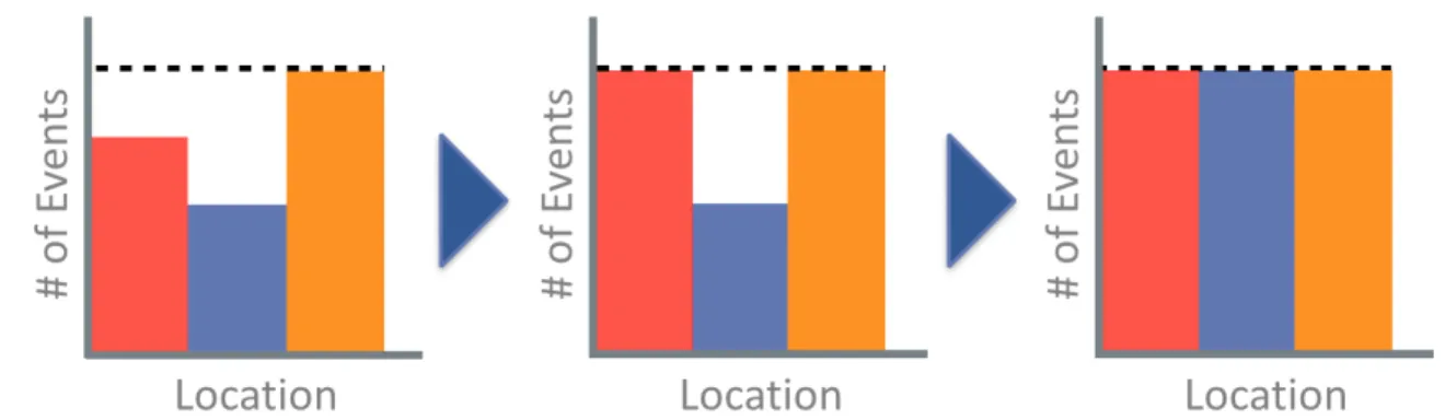
Figure 3-3: The water-filling algorithm described by Sec. 3.2.5 where the colors de-note three different discrete locations. The observation times for stations below the bottle-neck expected number of events (dashed black line) is increased until the (ap-proximate) expected number of observations at each station is equivalent.
3.2.5
Generating Balanced Policies that Consider
Approxima-tion Uncertainty
We build upon the method introduced in the previous section to generate a policy𝜋* 𝑘
that simultaneously satisfies the uncertainty constraint and balances attention given to all stations in approximately the minimum time possible. The key insight is that the value of 𝑡low
𝑖,𝑘 given by (3.8) acts as a lower bound on the observation time for
each station 𝑖∈ [𝑛] for satisfying the uncertainty constraint (see Lemma 2). We also leverage the following fact from [38] regarding the optimality of the balance objective for a policy 𝜋𝑘:
E[𝑁1(𝜋𝑘)] = · · · = E[𝑁𝑛(𝜋𝑘)]⇔ 𝜋𝑘∈ argmax 𝜋
ˆ
𝑓bal(𝜋). (3.9)
We use a combination of this result and the fact that any observation time sat-isfying 𝑡𝑖,𝑘 ≥ 𝑡low𝑖,𝑘 also satisfies the uncertainty constraint to arrive at an expression
for the optimal observation time for each station. In constructing the optimal policy 𝜋*
𝑘 = (𝑡 *
1,𝑘, . . . , 𝑡 *
𝑛,𝑘), we first identify the “bottleneck" value,𝑁max, which is computed
using the lower bounds for each 𝑡𝑖,𝑘, i.e., 𝑁max := max𝑖∈[𝑛]𝜆ˆ𝑖,𝑘𝑡low𝑖,𝑘 . Given (3.9), we
use the bottleneck value𝑁max to set the value of each observation time 𝑡*𝑖,𝑘
appropri-ately so that each𝑡*
the balance objective function. Namely, the optimal observation times for all sta-tions which constitute the per-cycle optimal policy 𝜋*
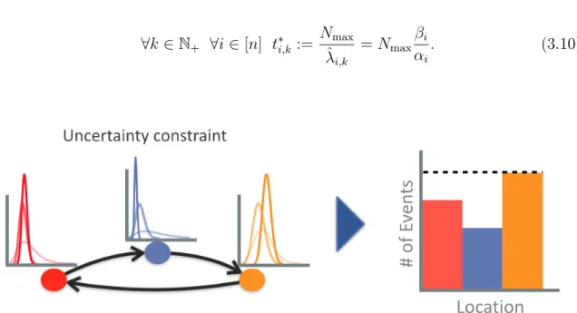
𝑘= (𝑡 * 1,𝑘, . . . , 𝑡 * 𝑛,𝑘) are computed individually: ∀𝑘 ∈ N+ ∀𝑖 ∈ [𝑛] 𝑡*𝑖,𝑘 := 𝑁max ˆ 𝜆𝑖,𝑘 =𝑁max 𝛽𝑖 𝛼𝑖 . (3.10)
Figure 3-4: A unified visualization of the components of our algorithm. The lower bounds for the observation times are generated according to the uncertainty constraint in order to ensure controlled decay of uncertainty (Left). The lower bounds are then utilized by the water-filling algorithm detailed in Sec. 3.2.5 to generate policies that are balanced. The conjunction of these two components culminates in monitoring policies that are conducive to both exploration and exploitation.
3.3
Analysis
The outline of results in this section is as follows: we begin by proving the uncertainty-reducing property and per-cycle optimality of policies generated by Alg. 2 with re-spect to the rate approximations. We present a probabilistic bound on posterior variance and error of our rate approximations with respect to the ground-truth rates by leveraging the properties of each policy. We use the previous results to establish a probabilistic bound on the per-cycle optimality of any arbitrary policy generated by Alg. 2 with respect to the ground-truth optimal solution of Problem 3.
Assumption 1. The parameters 𝜖 and 𝛿 are confined to the intervals (0, 2(1 + 2𝑒1/𝜋)−1) and (0, 1) respectively, i.e., 𝜖
∈ (0, 2(1 + 2𝑒1/𝜋)−1), 𝛿
∈ (0, 1).
A policy𝜋𝑘 is said to be approximately-optimal at cycle𝑘∈ N+ if𝜋𝑘is an optimal
solution to Problem 3 with respect to the rate approximations ˆ𝜆1,𝑘, . . . , ˆ𝜆𝑛,𝑘, i.e., if it
is optimal under the approximation of expectation: E[𝑁𝑖(𝜋𝑘)] ≈ ˆ𝜆𝑖,𝑘𝑡𝑖,𝑘 ∀𝑖 ∈ [𝑛]. In
contrast, a policy𝜋𝑘 is ground-truth optimal if it is an optimal solution to Problem 3
with respect to the ground-truth rates 𝜆1, . . . , 𝜆𝑛. For sake of notational brevity, we
introduce the function 𝑔 : R→ R denoting
𝑔(𝑥) := 1− 𝑒
−𝑥
max{︀2, 2√𝜋𝑥}︀ ,
and note the bound established by [31] for a Poisson random variable 𝑌 with mean 𝑚 and 𝑘 ∈ R+ such that 𝑘 ≥ 𝑚
P(︀(︀𝑌 ≤ 𝑘))︀ > 𝑔(︀𝐷KL(Pois(𝑚)|| Pois(𝑘)))︀. (3.11)
We begin by proving that each policy generated by Alg. 2 is optimal with respect to the per-cycle optimization problem (Problem 3).
Lemma 1 (Satisfaction of the uncertainty constraint). The observation time 𝑡low 𝑖,𝑘
given by (3.8) satisfies the uncertainty constraint (3.4) for any arbitrary station𝑖∈ [𝑛] and iteration 𝑘 ∈ N+.
Proof. We consider the left-hand side of (3.6) from Sect. 3.2 and marginalize over the unknown parameter 𝜆𝑖 ∈ R+: P(︀(𝑁𝑖(𝑡𝑖,𝑘)≤ 𝑘(𝑡𝑖,𝑘)|𝑋𝑖1:𝑘−1))︀ = ∫︁ ∞ 0 P(︀(𝑁𝑖(𝑡𝑖,𝑘)≤ 𝑘(𝑡𝑖,𝑘)|𝑋𝑖1:𝑘−1, 𝜆) )︀ P(︀(𝜆|𝑋𝑖1:𝑘−1))︀ 𝑑𝜆
where the probability is with respect to the random variable 𝑁𝑖(𝑡𝑖,𝑘) ∼ Pois(𝜆𝑡𝑖,𝑘)
credible interval constructed in Alg. 2, i.e. the interval (𝜆l 𝑖, 𝜆𝑢𝑖) satisfying ∀𝑖 ∈ [𝑛] ∀𝜆𝑖 ∈ R+ P(︀(𝜆l𝑖 > 𝜆𝑖|𝑋𝑖1:𝑘−1))︀ = P (︀(𝜆 u 𝑖 < 𝜆𝑖|𝑋𝑖1:𝑘−1))︀ = 𝜖 2, we establish the inequalities:
P(︀(𝑁𝑖(𝑡𝑖,𝑘)≤ 𝑘(𝑡𝑖,𝑘)|𝑋𝑖1:𝑘−1))︀ > ∫︁ 𝜆𝑢𝑖 0 P(︀(𝑁𝑖(𝑡𝑖,𝑘)≤ 𝑘(𝑡𝑖,𝑘)|𝑋𝑖1:𝑘−1, 𝜆) )︀ P(︀(𝜆|𝑋𝑖1:𝑘−1))︀ 𝑑𝜆 ≥ P(︀(𝑁𝑖(𝑡𝑖,𝑘)≤ 𝑘(𝑡𝑖,𝑘)|𝑋𝑖1:𝑘−1, 𝜆 𝑢 𝑖) )︀ ∫︁ 𝜆𝑢𝑖 0 P(︀(𝜆|𝑋𝑖1:𝑘−1))︀ 𝑑𝜆 = (1− 𝜖 2) P(︀(𝑁𝑖(𝑡𝑖,𝑘)≤ 𝑘(𝑡𝑖,𝑘)|𝑋 1:𝑘−1 𝑖 , 𝜆 𝑢 𝑖))︀ . (3.12)
where we utilized the fact that P(︀(︀𝑁𝑖(𝑡𝑖,𝑘)≤ 𝑘(𝑡𝑖,𝑘)|𝑋𝑖1:𝑘−1, 𝜆u𝑖)︀)︀ is monotonically
de-creasing with respect to 𝜆. By construction, 𝑡low
𝑖,𝑘 satisfies
𝐷KL(Pois(𝜆u𝑖𝑡low𝑖,𝑘 )|| Pois(𝑘(𝑡𝑖,𝑘low))) =𝑊𝜖 which yields 1− 𝑔(𝑊𝜖) = 1−2−𝜖𝜖 by definition
and thus by (3.11) we have:
P(︀(𝑁𝑖(𝑡low𝑖,𝑘 )≤ 𝑘(𝑡 low 𝑖,𝑘 )|𝑋 1:𝑘−1 𝑖 , 𝜆 u 𝑖))︀ > 1 − 𝑔(𝑊𝜖) = 1− 𝜖 2− 𝜖. Combining this inequality with the expression of (3.12) establishes the result.
Lemma 2 (Monotonicity of solutions satisfying (3.4)). For any arbitrary station 𝑖 ∈ [𝑛] and monitoring cycle 𝑘 ∈ N+, the observation time 𝑡𝑖,𝑘 satisfying 𝑡𝑖,𝑘 ≥ 𝑡low𝑖,𝑘,
where 𝑡low
𝑖,𝑘 is given by (3.8), satisfies the uncertainty constraint.
Theorem 1 (Per-cycle approximate-optimality of solutions). For any arbitrary cycle 𝑘 ∈ N+, the policy 𝜋𝑘* := (𝑡
*
1,𝑘, . . . , 𝑡 *
𝑛,𝑘) generated by Alg. 2 is an
approximately-optimal solution with respect to Problem 3.
Proof. By definition of (3.10), we have for any arbitrary cycle 𝑘 ∈ N+ and station
𝑖 ∈ [𝑛], 𝑡*
𝑖,𝑘 = 𝑁max/ˆ𝜆𝑖,𝑘 ≥ 𝑡low𝑖,𝑘 by definition of 𝑁max := max𝑖∈[𝑛]𝜆ˆ𝑖,𝑘𝑡low𝑖,𝑘. Applying
Lemma 2 and observing that
ˆ
implies that the uncertainty constraint is satisfied for all stations 𝑖 ∈ [𝑛] and that 𝜋*
𝑘 ∈ argmax𝜋𝑘
ˆ
𝑓bal(𝜋𝑘), which establishes the optimality of𝜋𝑘with respect to Problem
3.
Using the fact that each policy satisfies the uncertainty constraint, we establish probabilistic bounds on uncertainty, i.e. posterior variance, and rate approximations. Lemma 3 (Bound on posterior variance). After executing an arbitrary number of cycles 𝑘 ∈ N+, the posterior variance Var(𝜆𝑖|𝑋𝑖1:𝑘) is bounded above by 𝛿𝑘Var(𝜆𝑖)
with probability at least (1− 𝜖)𝑘, i.e.,
∀𝑖 ∈ [𝑛] ∀𝑘 ∈ N+ P(︀(︀Var(𝜆𝑖|𝑋𝑖1:𝑘)≤ 𝛿𝑘Var(𝜆𝑖)|𝑋𝑖1:𝑘)︀)︀ > (1 − 𝜖)𝑘
for all stations 𝑖∈ [𝑛] where Var(𝜆𝑖) :=𝛼𝑖,0/𝛽𝑖,02 is the prior variance.
Proof. Iterative application of the inequality Var(𝜆𝑖|𝑋𝑖1:𝑘) ≤ 𝛿Var(𝜆𝑖|𝑋𝑖1:𝑘−1) each
with probability 1− 𝜖 by the uncertainty constraint (3.4) yields the result.
Corollary 1 (Bound on variance of the posterior mean). After executing an arbitrary number of cycles 𝑘 ∈ N+, the variance of our approximation Var
(︀ˆ
𝜆𝑖,𝑘|𝑋𝑖1:𝑘−1
)︀ is bounded above by 𝛿𝑘−1Var(𝜆
𝑖) with probability greater than (1− 𝜖)𝑘−1, i.e.,
∀𝑖 ∈ [𝑛] P(︁(︀Var(ˆ𝜆𝑖,𝑘|𝑋𝑖1:𝑘−1)≤ 𝛿
𝑘−1Var(𝜆
𝑖)|𝑋𝑖1:𝑘−1
)︀)︁
> (1− 𝜖)𝑘−1.
Proof. Application of the law of total conditional variance and invoking Lemma 3 yields the result.
Theorem 2 (𝜉-bound on approximation error). For all 𝜉 ∈ R+ and cycles 𝑘 ∈ N+,
the inequality |ˆ𝜆𝑖,𝑘− 𝜆𝑖| < 𝜉 holds with probability at least (1 − 𝜖)𝑘−1(1−𝛿
𝑘−1Var(𝜆 𝑖) 𝜉2 ), i.e., ∀𝑖 ∈ [𝑛] P(︁(︀|ˆ𝜆𝑖,𝑘− 𝜆𝑖| < 𝜉|𝑋𝑖1:𝑘−1 )︀)︁ > (1− 𝜖)𝑘−1(︀1 − 𝛿𝑘−1Var(𝜆𝑖) 𝜉2 )︀.
Theorem 3 (∆-bound on optimality with respect to Problem 3). For any 𝜉𝑖 ∈ R+,
𝑖∈ [𝑛], 𝑘 ∈ N+, given that|ˆ𝜆𝑖,𝑘− 𝜆𝑖| ∈ (0, 𝜉𝑖) with probability as given in Theorem 2,
let 𝜎min :=∑︀𝑛𝑖=1(𝜆𝑖 − 𝜉𝑖)−1 and 𝜎max := ∑︀𝑛𝑖=1(𝜆𝑖+𝜉𝑖)−1. Then, the objective value
of the policy 𝜋*
𝑘 at iteration 𝑘 is within a factor of ∆ of the ground-truth optimal
solution, where ∆ := 𝜎min
𝜎max with probability greater than (1− 𝜖)
𝑛(𝑘−1)(︀1 −𝛿𝑘−1Var(𝜆 𝑖)
𝜉2
)︀𝑛 . Proof. Note that for any arbitrary total observation time 𝑇 ∈ R+, a policy 𝜋𝑘 =
(𝑡* 1,𝑘, . . . , 𝑡*𝑛,𝑘) satisfying ∀𝑖 ∈ [𝑛] 𝑡*𝑖,𝑘 := 𝑇 𝜆𝑖 ∑︀𝑛 𝑙=1 1 𝜆𝑙 . (3.13)
optimizes the balance objective function ˆ𝑓bal [38]. Using the fact that |ˆ𝜆𝑖,𝑘 − 𝜆𝑖| < 𝜉𝑖
with probability given by Theorem 2, we arrive at the following inequality for ˆ𝑓bal(𝜋𝑘*)
ˆ 𝑓bal(𝜋*𝑘)> 𝑇 ∑︀𝑛 𝑙=1(𝜆𝑖+𝜉𝑙)−1 𝑛𝑇 ∑︀𝑛 𝑙=1(𝜆𝑙−𝜉𝑙)−1 = ∑︀𝑛 𝑙=1(𝜆𝑙− 𝜉𝑙) −1 𝑛∑︀𝑛 𝑙=1(𝜆𝑙+𝜉𝑙)−1
with probability at least (1− 𝜖)𝑛(𝑘−1)(︀1 − 𝛿𝑘−1Var(𝜆𝑖)
𝜉2
)︀𝑛 .
3.4
Results
We evaluate the performance of Alg. 1 in two simulated scenarios modeled after real-world inspired monitoring tasks: (i) a synthetic simulation in which events at each station precisely follow a station-specific Poisson process and (ii) a scenario simulated in Armed Assault (ARMA) [7], a military simulation game, involving detections of suspicious agents. We note the statistics do not match our assumed Poisson model, and yet our algorithm performs well compared to other approaches. We compare Alg. 1 to the following monitoring algorithms:
1. Equal Time, Min. Delay (ETMD): computes the total cycle time to minimize latency 𝑇obs [38] and partitions 𝑇obs evenly across all stations.
generates policies that minimize latency and maximize observation balance.
3. Incremental Search, Bal. Events (ISBE): generates policies to maximize balance that increase in length by a fixed amount ∆obs ∈ R+ after each cycle.
0
100 200 300 400 500 600
Time (minutes)
0.00
0.03
0.06
0.09
0.12
0.15
0.18
0.21
0.24
0.27
0.30
0.33
Observation Balance
(a) Balance objective value
0
100 200 300 400 500 600
Time (minutes)
0
5
10
15
20
25
30
35
Percentage of Events Observed
(b) Percentage of events observed
0
100 200 300 400 500 600
Time (minutes)
0
40
80
120
160
200
240
280
320
Percent Approximation Error
(c) Percentage error
0
100 200 300 400 500 600
Time (minutes)
0
10
20
30
40
50
Mean Squared Error (MSE)
(d) Mean squared error (MSE)
Figure 3-5: Results of the synthetic simulation averaged over 10,000 trials that char-acterize and compare our algorithm to the four monitoring algorithms in randomized environments containing three discrete stations.
4. Oracle Algorithm (Oracle Alg.): an omniscient algorithm assuming perfect knowledge of ground-truth rates and monitoring time𝑇maxwhere each
observa-tion time is generated according to (3.13).
3.4.1
Synthetic Scenario
We consider the monitoring scenario involving the surveillance of events in three discrete stations over a monitoring period of 10 hours. We characterize the average performance of each monitoring algorithm with respect to 10,000 randomly generated problem instances with the following statistics:
1. Prior hyper-parameters: 𝛼𝑖,0 ∼ Uniform(1, 20) and 𝛽𝑖,0 ∼ Uniform(0.75, 1.50).
2. Rate parameter of each station: 𝜇𝜆𝑖 = 2.23 and 𝜎𝜆𝑖 = 1.02 events per minute.
3. Initial percentage error of the rate estimate 𝜆𝑖,0, denoted by 𝜌𝑖: 𝜇𝜌𝑖 = 358.29%
and 𝜎𝜌𝑖 = 221.32%.
4. Travel cost from station 𝑖 to another 𝑗: 𝜇𝑑𝑖,𝑗 = 9.97 and 𝜎𝑑𝑖,𝑗 = 2.90 minutes.
where𝜇 and 𝜎 refer to standard deviation and variance of each parameter respectively and the transient events at each station 𝑖 ∈ [𝑛] are simulated precisely according to Pois(𝜆𝑖).
The performance of each algorithm with respect to the the monitoring objectives defined in Sect. 3.1 is shown in Figs. 3-5a and 3-5b respectively. The figures show that our algorithm is able to generate efficient policies that enable the robot to observe sig-nificantly more events that achieve a higher balance in comparison to those computed by other algorithms (with exception of Oracle Alg.) at all times of the monitoring process. Figs. 3-5c and 3-5d depict the efficiency of each monitoring algorithm in rapidly learning the events’ statistics and generating accurate approximations. The error plots show that our algorithm achieves lower measures of error at any given time in comparison to those of other algorithms and supports our method’s practical efficiency in generating exploratory policies conducive to rapidly obtaining accurate
approximations of event statistics. Figs. 3-5a-3-5d show our algorithm’s dexterity in balancing the inherent trade-off between exploration vs. exploitation.
Figure 3-6: Viewpoints from two stations in the ARMA simulation of the yellow backpack scenario. Agents wearing yellow backpacks whose detections are of interest appear in both figures.
3.4.2
Yellow Backpack Scenario
In this subsection, we consider the evaluation of our monitoring algorithm in a real-world inspired scenario, labeled the yellow backpack scenario, that entails monitoring of suspicious events that do not adhere to the assumed Poisson model (Sect. 3.1). Using the military strategy game ARMA, we simulate human agents that wander
around randomly in a simulated town. A subset of the agents wear yellow backpacks (see Fig. 3-6). Under this setting, our objective is to optimally monitor the yellow backpack-wearing agents using three predesignated viewpoints, i.e. stations. We con-sidered a monitoring duration of 5 hours under the following simulation configuration:
0
50 100 150 200 250 300
Time (minutes)
0.00
0.03
0.06
0.09
0.12
0.15
0.18
0.21
0.24
0.27
0.30
0.33
Observation Balance
(a) Balance objective value
0
50 100 150 200 250 300
Time (minutes)
0
5
10
15
20
25
30
35
40
Percentage of Events Observed
(b) Percentage of events observed
0
50 100 150 200 250 300
Time (minutes)
0
20
40
60
80
100
120
Percent Approximation Error
(c) Percentage error
0
50 100 150 200 250 300
Time (minutes)
0
50
100
150
200
250
300
350
400
450
Mean Squared Error (MSE)
(d) Mean squared error (MSE)
Figure 3-7: The performance of each monitoring algorithm evaluated in the ARMA-simulated yellow backpack scenario.
1. Environment dimensions: 250 meters x 250 meters (62, 500 meters2).
2. Number of agents with a yellow backpack: 10 out of 140 (≈ 7.1% of agents). 3. Travel cost (minutes): 𝑑1,2 = 3, 𝑑2,3 = 2, 𝑑3,1 = 12.
We used the Faster Region-based Convolutional Neural Network (Faster R-CNN, [29]) for recognizing yellow backpack-wearing agents in real-time at a frequency of 1 Hertz. We ran the simulation for a sufficiently long time in order to obtain estimates for the respective ground-truth rates of 23.3, 20.3, and 18.5 yellow backpack recognitions per minute, which were used to generate Figs. 3-7c and 3-7d. The results of the yellow backpack scenario, shown in Figs. 3-7a-3-7d, tell the same story as did the results of the synthetic simulation. We note that at all instances of the monitoring process, our approach that leverages uncertainty estimates outperforms others in generating bal-anced policies conducive to efficiently observing more events and obtaining accurate rate approximations.
Chapter 4
Unknown, Dynamic Environments
In this chapter we relax the assumption of static event statistics and consider the problem of persistent monitoring in unknown, dynamic environments.
4.1
Problem Definition
Let there be 𝑛 ∈ N+ discrete stations in the environment where transient events of
interest occur according to inhomogeneous Poisson processes. The temporal variations at each station 𝑖 ∈ [𝑛] are governed by an integrable rate function 𝜆𝑖 : R≥0 → R+
that is station-specific and independent of those of other stations. We assume that the rate functions can exhibit an unbounded number of abrupt changes, however, we require that the total variation of each function 𝜆𝑖 within the time horizon 𝑇 ∈ R+
be bounded by a variation budget 𝑉𝑇 ∈ R+ [5], i.e.,
sup 𝑃 ∈𝒫 𝑛𝑝−1 ∑︁ 𝑗=1 max 𝑖∈[𝑛] ⃒ ⃒𝜆𝑖(𝑝𝑗+1)− 𝜆𝑖(𝑝𝑗) ⃒ ⃒≤ 𝑉𝑇, (4.1)
where 𝒫 = {︀𝑃 = {𝑝1, . . . , 𝑝𝑛𝑃} | 𝑃 is a partition of [0, 𝑇 ]}︀. We note that since our
problem is intimately linked with the MAB problem, we address the case of a known surveillance duration 𝑇 as is common in MAB literature.
We assume that there exists a travel cost,𝑐 : [𝑛]×[𝑛] → R≥0, associated with going
stationary to make accurate measurements, the robot cannot make observations while traveling. Our overarching monitoring objective is to generate an optimal sequence of station-time pairs that dictates the appropriate station visit order and respective observation windows in order to maximize the number of sighted events.
More formally, a policy𝜋 =(︀(𝑠1, 𝑡1), . . . , (𝑠𝑚, 𝑡𝑚))︀ is a sequence of 𝑚 ∈ N+ordered
pairs where each ordered pair, (𝑠, 𝑡), denotes an observation window of 𝑡∈ R≥0 time
at station 𝑠∈ [𝑛]. For any non-negative reals 𝑎, 𝑏 such that 𝑎 ≤ 𝑏, let 𝑁𝑖(𝑎, 𝑏] denote
the random number of events that occur in the time interval (𝑎, 𝑏] at station 𝑖∈ [𝑛]. It follows then that E[︀𝑁𝑖(𝑎, 𝑏]
]︀
= ∫︀𝑎𝑏𝜆𝑖(𝜏 ) 𝑑𝜏 by definition of an inhomogeneous
Poisson process at each station 𝑖. The expected number of events obtained for any policy 𝜋 = (︀(𝑠1, 𝑡1), . . . , (𝑠𝑚, 𝑡𝑚))︀ constrained by the total surveillance time 𝑇 can
then be computed as follows:
E[𝑁 (𝜋, 𝑇 )] := 𝑚 ∑︁ 𝑗=1 ∫︁ 𝑜𝑗(𝜋)+𝑡𝑗 𝑜𝑗(𝜋) 𝜆𝑠𝑗(𝜏 ) 𝑑𝜏, (4.2)
where 𝑜𝑗(𝜋) denotes the start of the 𝑗th observation window, i.e., 𝑜1(𝜋) = 0 and for
any integral value𝑗 > 1,
𝑜𝑗(𝜋) := 𝑗−1
∑︁
𝑘=1
𝑡𝑘+𝑐(𝑠𝑘, 𝑠𝑘+1).
Our notion of weak regret is defined relative to the maximum number of expected events, 𝑁*
𝑇 at a single best station after an allotted monitoring time of 𝑇 ∈ R+:
𝑁𝑇* = max
𝑖∈[𝑛]E[︀𝑁𝑖(0, 𝑇 ]]︀ = max𝑖∈[𝑛]
∫︁ T 0
𝜆𝑖(𝜏 ) 𝑑𝜏.
We seek to generate policies that minimize the expected regret with respect to the quantity𝑁*
𝑇. We let𝑅(𝜋, 𝑇 ) denote the regret accrued by policy 𝜋 =(︀(𝑠1, 𝑡1), . . . , (𝑠𝑚, 𝑡𝑚)
)︀ after time𝑇
and define our optimization problem with respect to the expectation of 𝑅(𝜋, 𝑇 ). Problem 4 (Persistent Surveillance Problem). Compute the optimal monitoring pol-icy, 𝜋* =(︀(𝑠*
1, 𝑡*1), . . . , (𝑠*𝑚, 𝑡*𝑚))︀, that minimizes the expected regret with respect to the
allotted monitoring time 𝑇
𝜋* = argmin
𝜋 E[𝑅(𝜋, 𝑇 )].
(4.4)
In what follows, we seek to minimize a long-term variant of Eqn. 4.4. We define the long-run average optimal policy as
Definition 1 (Long-run Average Optimal Policy). A policy𝜋 =(︀(𝑠1, 𝑡1), . . . , (𝑠𝑚, 𝑡𝑚)
)︀ is called a long-run average optimal policy if and only if
lim sup 𝑇 →∞ E[𝑅(𝜋, 𝑇 )] 𝑇 = E[𝑁𝑇*]− E[𝑁(𝜋, 𝑇 )] 𝑇 ≤ 0. (4.5)
4.2
Methods
In this section, we describe the intuition behind our approach, and present a moni-toring algorithm (Alg. 3). Our approach trades off exploration and exploitation by leveraging information gained within bounded time steps. Specifically, we partition our alloted time into equal length intervals called epochs. Within each epoch we rea-son about the currently known best station and attempt to cleverly remove stations that are suboptimal with high probability. By removing suboptimal stations, future passes through the list of remaining stations are expected to yield better long-term rewards and require less time to be spent on traveling relative to observing stations. The algorithm begins by computing the length of each epoch, 𝜏 , as a function of the total time 𝑇 , variation budget 𝑉𝑇, and maximum travel time between each
station 𝑇travel = max𝑖,𝑗∈[𝑛]:𝑖̸=𝑗𝑐(𝑖, 𝑗). The variables 𝑁𝑖 and 𝑇𝑖, denoting the total
number of observations and the total time spent at station𝑖 respectively, are reset at the beginning of each epoch. Discarding out-dated information in this way enables us to balance remembering and forgetting by computing the average rate, ˆ𝜆𝑖 = 𝑁𝑖/𝑇𝑖,
Figure 4-1: An example instance of our algorithm, depicting the partitioning of the monitoring period𝑇 into epochs of length 𝜏 . Within each epoch, the robot executes our variant of the Upper Confidence Bounds (UCB) algorithm to balance exploration and exploitation. Information obtained from prior epochs is purposefully discarded at the start of each epoch in order to adapt to the temporal variations in the environment.
for each station using only information obtained within that epoch. For each epoch, our method employs an algorithm based on the Improved UCB Algorithm [4] and seeks to balance the inherent exploration/exploitation trade-off.
4.3
Analysis
In this section, we present a regret bound analysis proving that the policy𝜋 generated by Alg. 3 is long-run average optimal with respect to our definition of weak regret. To establish our result, we proceed by bounding the total regret in each epoch of length 𝜏 , and then sum the regret over all ⌈𝑇
𝜏⌉ epochs to obtain an upper bound on
the entire monitoring horizon of length 𝑇 .
4.3.1
Preliminaries
Assumption 2 (Bounded Rates). For a given time horizon𝑇 ∈ R+, the rate
param-eters ∀𝑖 ∈ [𝑛] 𝜆𝑖 : R≥0 → R+ are bounded above by a known constant 𝜆max.
Define a stage indexed by 𝑚 ∈ N as the completion of the inner while loop of Alg. 3 (i.e., execution of lines 13-30) and denote the partition of the time horizon 𝑇 into𝑘 =⌈𝑇
𝜏⌉ epochs as 𝜏1, . . . , 𝜏𝑘 of length 𝜏 each (with the possible exception of 𝜏𝑘).
For a given stage𝑚, we define ˜∆(𝑚), 𝑇obs(𝑚), 𝑆(𝑚), and 𝜉(𝑚) as the values of each
variable at stage 𝑚 (see Alg. 3). Let 𝑤𝑖,0, . . . , 𝑤𝑖,𝑚 be the 𝑚 + 1 ∈ N observation
windows at station𝑖∈ [𝑛], where each observation window 𝑤𝑖,𝑗 is defined by the time
interval (𝑎𝑖,𝑗, 𝑏𝑖,𝑗). Note that ∑︀𝑚𝑗=0(𝑏𝑖,𝑗− 𝑎𝑖,𝑗) =𝑇obs(𝑚).
For an arbitrary epoch𝜏𝑗, we let ˆ𝜆𝑖(𝑚) denote the sample mean of the rate
param-eter and let ¯𝜆𝑖(𝑚) denote the ground-truth mean rate after observing at station 𝑖 for
𝑚 stages. We define ¯𝜆𝑖 to denote the average rate of a station over the specific epoch
𝜏𝑗 (that is clear from the context) and let ¯𝜆* = max𝑖∈[𝑛]¯𝜆𝑖 denote the epoch-specific
optimal rate of the best station*. Finally, we let ∆𝑖 = ¯𝜆*− ¯𝜆𝑖 denote the difference
Algorithm 3: Dynamic Upper Confidence Bound Monitoring Algorithm
Input: Time horizon 𝑇 , variation budget 𝑉𝑇, number of stations 𝑛, and travel
costs 𝑐 : [𝑛]× [𝑛] → R≥0.
Effect: Monitors locations of interest for 𝑇 time.
1 𝑇travel ← max𝑖,𝑗∈[𝑛]:𝑖̸=𝑗𝑐(𝑖, 𝑗);
2 // Compute the length of each epoch 3 𝜏 ← (𝑛𝜆max𝑇 /𝑉𝑇)
2 3;
4 while 𝑡current ≤ 𝑇 do
5 // Initialize parameters, discarding all previously obtained information
from previous epochs
6 𝑇𝑖 ← 0 ∀𝑖 ∈ [𝑛]; 𝑁𝑖 ← 0 ∀𝑖 ∈ [𝑛]; 7 // Initialize the set of all station indices 8 𝑆 ← {1, . . . , 𝑛};
9 ∆˜ ← 𝜆max;
10 // Determine the end point of the current epoch 11 𝑇end← 𝑡current+𝜏 ;
12 while 𝑡current ≤ 𝑇end do
13 // Compute the goal observation time 14 𝑇obs ← 8𝜆maxlog (︀ 𝜏 ˜Δ2)︀ 3 ˜Δ2 ; 15 if |𝑆| > 1 then
16 for 𝑖* ∈ 𝑆 such that 𝑇𝑖* < 𝑇obs do
17 𝑡𝑖* ← min{︀𝑇end− 𝑡current, 𝑇obs − 𝑇𝑖*}︀;
18 Observe at station 𝑖* for 𝑡𝑖* time;
19 𝑇𝑖* ← 𝑇𝑖* +𝑡𝑖*;
20 else
21 // Only one station remains in 𝑆 22 𝑡𝑖* ← 𝑇end− 𝑡current;
23 Observe at the sole station 𝑖* ∈ 𝑆 until 𝑇end; 24 𝑇𝑖* ← 𝑇𝑖* +𝑡𝑖*;
25 // Identify and remove suboptimal stations 26 𝜉 ← √︂ 8𝜆maxlog (︀ 𝜏 ˜Δ2)︀ 3𝑇obs ; 27 𝜆ˆ* ← max𝑖∈𝑆𝜆ˆ𝑖− 𝜉; 28 𝐵 ← {𝑖 ∈ 𝑆 | ˆ𝜆𝑖+𝜉 < ˆ𝜆*}; 29 𝑆 ← 𝑆 ∖ 𝐵; 30 ∆˜ ← Δ˜2;
Fact 1 (Chernoff Bounds). Let𝑋∼ Poisson(𝜆), then the following holds for 𝜉 ∈ R≥0: P (𝑋 > 𝜆 + 𝜉)≤ exp (︂ −𝜉 2 2𝜆𝜓(𝜉/𝜆) )︂ ,
and for 𝜉∈ [0, 𝜆max]
P (𝑋 < 𝜆− 𝜉) ≤ exp (︂ −𝜉 2 2𝜆𝜓(−𝜉/𝜆) )︂ ≤ exp (︂ −𝜉 2 2𝜆 )︂ , where 𝜓(𝑥) = (1 +𝑥) log(1 + 𝑥)− 𝑥 𝑥2/2 ≥ (1 + 𝑥/3) −1 .
Lemma 4 (Concentration Inequalities). For any station 𝑖 ∈ [𝑛] and arbitrary se-quence of observation windows 𝑤𝑖,0, . . . , 𝑤𝑖,𝑚 such that 𝑇obs(𝑚) =
∑︀𝑚 𝑗=0(𝑏𝑖,𝑗 − 𝑎𝑖,𝑗) and 𝜉 ∈ R≥0: P(︁ˆ𝜆𝑖(𝑚) > ¯𝜆𝑖(𝑚) + 𝜉 )︁ ≤ exp (︂ −3𝑇obs(𝑚)𝜉 2 8𝜆max )︂
and for 𝜉∈ [0, 𝜆max]
P(︁ˆ𝜆𝑖(𝑚) < ¯𝜆𝑖(𝑚)− 𝜉 )︁ ≤ exp (︂ −3𝑇obs(𝑚)𝜉 2 8𝜆max )︂ .
Proof. Let𝑁 be the random variable denoting the number of events observed during the observation windows summing up to a total of𝑇obs time. Then, it follows by
defi-nition of a Poisson process that 𝑁 ∼ Poisson(¯𝜆𝑖𝑇obs) and thus by the aforementioned
Chernoff bounds, we have for 𝜉∈ R≥0:
P(︁ˆ𝜆𝑖 ≤ ¯𝜆𝑖+𝜉 )︁ = P (𝑁 > E[𝑁 ] + 𝜉𝑇obs) ≤ exp(︂ 𝑇obs𝜉 2 2¯𝜆𝑖 𝜓(𝜉/¯𝜆𝑖) )︂ and for 𝜉∈ [0, ¯𝜆𝑖]: P(︁ˆ𝜆𝑖 ≤ ¯𝜆𝑖− 𝜉 )︁ ≤ exp(︂ 𝑇obs𝜉 2 2¯𝜆𝑖 𝜓(−𝜉/¯𝜆𝑖) )︂ .
Now, note that 𝜉 ≤ 𝜆max by definition, and consider the expression 𝑇obs𝜉 2 2¯𝜆𝑖 𝜓(𝜉/¯𝜆𝑖): 𝑇obs𝜉2 2¯𝜆𝑖 𝜓(𝜉/¯𝜆𝑖)≥ 𝑇obs𝜉2 2¯𝜆𝑖 𝜓(𝜉/¯𝜆𝑖) ≥ 𝑇obs𝜉 2 2¯𝜆𝑖 (︂ 3¯𝜆𝑖 3¯𝜆𝑖+𝜉 )︂ ≥ 3𝑇obs𝜉 2 8𝜆max
where we used the inequality 𝜓(𝑥) ≥ (1 + 𝑥/3)−1 mentioned in Fact 1. The result
above implies that
exp (︂ −𝑇obs𝜉 2 2𝜆 𝜓(𝜉/¯𝜆𝑖) )︂ ≤ exp (︂ −3𝑇obs𝜉 2 8𝜆max )︂ . (4.6)
Application of (4.6) yields the desired result:
∀𝜉 ∈ R≥0 P(︁ˆ𝜆𝑖 > ¯𝜆𝑖+𝜉 )︁ ≤ exp (︂ −3𝑇obs𝜉 2 8𝜆max )︂
and for 𝜉∈ [0, 𝜆max]:
P(︁ˆ𝜆𝑖 > ¯𝜆𝑖+𝜉 )︁ ≤ exp (︂ −𝑇obs𝜉 2 2¯𝜆𝑖 )︂ ≤ exp (︂ −3𝑇obs𝜉 2 8𝜆max )︂
4.3.2
Regret over an epoch
We decompose the total expected regret over an arbitrary epoch 𝜏𝑗 of length 𝜏 ,
E[𝑅(𝜋, 𝜏 )], and consider the regret incurred by observing and traveling separately, i.e., E[𝑅(𝜋, 𝜏 )] = E[𝑅obs(𝜋, 𝜏 )] + E[𝑅travel(𝜋, 𝜏 )].
Lemma 5 (Regret over an Epoch). The per-epoch expected observation regret of our algorithm, E[𝑅obs(𝜋, 𝜏 )], with respect to an arbitrary epoch 𝑗 of length 𝜏 and with
variation budget 𝑉𝑗 is at most (∆ +𝑉𝑗)𝜏 + ∑︁ 𝑖∈ℬ (︂ 1024 ∆𝑖 + 2560𝜆maxlog (𝜏 ∆ 2 𝑖/64) 3∆𝑖 )︂ , where ∆ = max{︁4𝑉𝑗, √︁ 8 exp(1−3/(5𝜆max)) 𝜏 }︁ and ℬ = {𝑖 ∈ [𝑛] | ∆𝑖 > ∆}.
Proof. Our proof employs results established in, and follows a similar structure as the proof given by Auer [4] and [5]. Let 𝑉𝑗 denote the total variation in the rates during
epoch 𝑗, i.e., 𝑉𝑗 = sup 𝑃 ∈𝒫𝑗 𝑛𝑝−1 ∑︁ 𝑘=1 max 𝑖∈[𝑛] ⃒ ⃒𝜆𝑖(𝑝𝑘+1)− 𝜆𝑖(𝑝𝑘) ⃒ ⃒, (4.7)
where 𝒫𝑗 is a partition of epoch 𝜏𝑗. Summing over all epochs 𝑗 = 1, . . . ,⌈𝑇𝜏⌉, note
that ∑︀⌈𝑇 /𝜏 ⌉
𝑗=1 𝑉𝑗 ≤ 𝑉𝑇.
Let 𝑚𝑖 = min{𝑚 : ˜∆(𝑚) < ∆𝑖/8} denote the first stage index in which our guess
˜
∆(𝑚) is close to the actual difference in the rates for stations 𝑖 ∈ 𝑆. The following inequalities follow by definition
˜ ∆(𝑚𝑖) = 𝜆max 2𝑚𝑖 < ∆𝑖 8 ≤ 2 ˜∆(𝑚𝑖) = 2𝜆max 2𝑚𝑖 (4.8) and 𝜉(𝑚𝑖) = ⎯ ⎸ ⎸ ⎷8𝜆max log(︁𝜏 ˜∆2(𝑚 𝑖) )︁ 3𝑇obs(𝑚𝑖) = ˜∆(𝑚𝑖)< ∆𝑖/8.
We will consider bounding the regret incurred by monitoring clearly suboptimal loca-tions, i.e., ℬ = {𝑖 ∈ 𝑆 | ∆𝑖 > ∆}, instead of monitoring the optimal station *, where
∆ = max{4𝑉𝑗,
√︁
8 exp(1−3/(5𝜆max))
𝜏 }.
Case 1 (At stage 𝑚𝑖, there exists a sub-optimal station 𝑖 ∈ 𝑆(𝑚𝑖) and the optimal
station* is in 𝑆(𝑚𝑖)). We will proceed by finding an upper bound for the probability
Consider the following inequalities for some stage 𝑚 ˆ 𝜆𝑖(𝑚)≤ ¯𝜆𝑖(𝑚) + 𝜉(𝑚) (4.9) ˆ 𝜆*(𝑚)≥ ¯𝜆* (𝑚)− 𝜉(𝑚). (4.10)
If conditions (4.9) and (4.10) hold at stage 𝑚 = 𝑚𝑖 under the assumption that
* ∈ 𝑆(𝑚𝑖), then it follows that 𝑖 will be removed from 𝑆(𝑚𝑖) at stage 𝑚𝑖
ˆ 𝜆𝑖(𝑚𝑖) +𝜉(𝑚𝑖)≤ ¯𝜆𝑖(𝑚𝑖) + 2𝜉(𝑚𝑖) by (4.9) ≤ ¯𝜆𝑖+𝑉𝑗+ 2𝜉(𝑚𝑖) by (4.7) < ¯𝜆𝑖+ ∆𝑖− 𝑉𝑗− 2𝜉(𝑚𝑖) ≤ ¯𝜆*− 𝑉𝑗− 2𝜉(𝑚𝑖) ≤ ¯𝜆*(𝑚𝑖)− 2𝜉(𝑚𝑖) by (4.7) ≤ ˆ𝜆*(𝑚𝑖)− 𝜉(𝑚𝑖) by (4.10)
where we used the fact that ∆𝑖 > 2𝑉𝑗+ 4𝜉(𝑚𝑖).
Using Lemma 4, the probability that either (4.9) or (4.10) does not hold is as follows. P(︁ˆ𝜆𝑖(𝑚𝑖)> ¯𝜆𝑖(𝑚𝑖) +𝜉(𝑚𝑖) )︁ ≤ 1 𝜏 ˜∆2(𝑚 𝑖) ,
and similarly for condition (4.10)
P(︁ˆ𝜆*(𝑚𝑖)< ¯𝜆*(𝑚𝑖)− 𝜉(𝑚𝑖)
)︁
≤ 1
𝜏 ˜∆2(𝑚 𝑖)
By the union bound, the probability that the sub-optimal station is not eliminated in stage 𝑚𝑖 (or before) is bounded above by 𝜏 ˜Δ22
𝑖(𝑚𝑖). Taking the sum of conditional