Publisher’s version / Version de l'éditeur:
Vous avez des questions? Nous pouvons vous aider. Pour communiquer directement avec un auteur, consultez la première page de la revue dans laquelle son article a été publié afin de trouver ses coordonnées. Si vous n’arrivez pas à les repérer, communiquez avec nous à [email protected].
Questions? Contact the NRC Publications Archive team at
[email protected]. If you wish to email the authors directly, please see the first page of the publication for their contact information.
https://publications-cnrc.canada.ca/fra/droits
L’accès à ce site Web et l’utilisation de son contenu sont assujettis aux conditions présentées dans le site LISEZ CES CONDITIONS ATTENTIVEMENT AVANT D’UTILISER CE SITE WEB.
Journal of the American Water Resources Association, 55, 6, pp. 1401-1424,
2019-09-03
READ THESE TERMS AND CONDITIONS CAREFULLY BEFORE USING THIS WEBSITE. https://nrc-publications.canada.ca/eng/copyright
NRC Publications Archive Record / Notice des Archives des publications du CNRC :
https://nrc-publications.canada.ca/eng/view/object/?id=2a329ee7-378e-4bfc-b1ec-ebbae228579c
https://publications-cnrc.canada.ca/fra/voir/objet/?id=2a329ee7-378e-4bfc-b1ec-ebbae228579c
Archives des publications du CNRC
This publication could be one of several versions: author’s original, accepted manuscript or the publisher’s version. / La version de cette publication peut être l’une des suivantes : la version prépublication de l’auteur, la version acceptée du manuscrit ou la version de l’éditeur.
For the publisher’s version, please access the DOI link below./ Pour consulter la version de l’éditeur, utilisez le lien DOI ci-dessous.
https://doi.org/10.1111/1752-1688.12792
Access and use of this website and the material on it are subject to the Terms and Conditions set forth at
Phosphorus and nitrogen transport in the binational Great Lakes Basin
estimated using SPARROW watershed models
Robertson, Dale M.; Saad, David A.; Benoy, Glenn A.; Vouk, Ivana;
Schwarz, Gregory E.; Laitta, Michael T.
Phosphorus and Nitrogen Transport in the Binational Great Lakes Basin Estimated Using
SPARROW Watershed Models
Dale M. Robertson, David A. Saad, Glenn A. Benoy, Ivana Vouk, Gregory E. Schwarz, and Michael T. Laitta
Research Impact Statement: As part of a binational effort, SPARROW watershed models were developed for the entire Great Lakes Basin and used to determine the amount and sources of phosphorus and nitrogen input to each lake.
ABSTRACT: Eutrophication problems in the Great Lakes are caused by excessive nutrient inputs (primarily phosphorus, P, and nitrogen, N) from various sources throughout its basin. In developing protection and restora-tion plans, it is important to know where and from what sources the nutrients originate. As part of a binarestora-tional effort, Midcontinent SPARROW (SPAtially Referenced Regression On Watershed attributes) models were devel-oped and used to estimate P and N loading from throughout the entire basin based on nutrient inputs similar to 2002; previous SPARROW models only estimated U.S. contributions. The new models have a higher resolution (~2-km2 catchments) enabling improved descriptions of where nutrients originate and the sources at various spatial scales. The models were developed using harmonized geospatial datasets describing the stream network, nutrient sources, and environmental characteristics affecting P and N delivery. The models were calibrated using loads from sites estimated with ratio estimator and regression techniques and additional statistical approaches to reduce spatial correlation in the residuals and have all monitoring sites equally influence model development. SPARROW results, along with interlake transfers and direct atmospheric inputs, were used to quantify the entire P and N input to each lake and describe the importance of each nutrient source. Model results can be used to compare loading and yields from various tributaries and jurisdictions.
(KEYWORDS: watershed modeling; loading; nutrients; spatially referenced regression.)
INTRODUCTION
The Laurentian Great Lakes is the largest fresh-water system in the world, with nearly 10% of the United States (U.S.) population and 30% of the Cana-dian population in its watershed (USEPA 2018a). The
Great Lakes receive nutrients from many tributaries draining areas ranging from pristine forests to inten-sively farmed areas and large urban centers, which results in nutrient input from these tributaries being extremely variable (Robertson and Saad 2011). Exces-sive nutrient inputs have caused eutrophication prob-lems to various degrees and at scales ranging from
Paper No. JAWRA-18-0103-P of the Journal of the American Water Resources Association (JAWRA). Received July 23, 2018; accepted July 11, 2019. © 2019 The Authors. Journal of the American Water Resources Association published by Wiley on behalf of the American Water Resources Association. This article is a U.S. Government work and is in the public domain in the USA.. This is an open access article under the terms of the Creative Commons Attribution-NonCommercial-NoDerivs License, which permits use and distribution in any medium, provided the original work is properly cited, the use is non-commercial and no modifications or adaptations are made. Discussions are open until six months from issue publication.
Upper Midwest Water Science Center (Robertson, Saad), U.S. Geological Survey, Middleton, Wisconsin, USA; Canadian Section (Benoy), International Joint Commission, Ottawa, Ontario, CAN; Ocean, Coastal and River Engineering (Vouk), National Research Council Canada, Ottawa, Ontario, CAN; National Center (Schwarz), U.S. Geological Survey, Reston, Virginia, USA; and U.S. Section (Laitta), International Joint Commission, Washington D.C., USA (Correspondence to Robertson: [email protected]).
Citation: Robertson, D.M., D.A. Saad, G.A. Benoy, I. Vouk, G.E. Schwarz, and M.T. Laitta. 2019. “Phosphorus and Nitrogen Transport in
the Binational Great Lakes Basin Estimated Using SPARROW Watershed Models.” Journal of the American Water Resources Association 1– 24. https://doi.org/10.1111/1752-1688.12792.
bays around the Great Lakes (e.g., Green Bay in Lake Michigan, Maccoux et al. 2013, and Bay of Quinte in Lake Ontario, Minns et al. 2011) to most of Lake Erie (Watson et al. 2016). Because of the degra-dation in water quality, several national and bina-tional efforts have been conducted to reduce nutrient loading to the Great Lakes, such as the binational Great Lakes Water Quality Agreement (GLWQA), the Great Lakes Restoration Initiative led by the U.S. Environmental Protection Agency (USEPA 2018b), and the Great Lakes Nutrient Initiative led by Envi-ronment and Climate Change Canada (ECCC 2013). As part of the GLWQA (1978), phosphorus (P) loading targets were established for each lake (Table 1). These targets are currently under review as an annex to the GLWQA.
In developing nutrient reduction strategies and restoration plans, it is important to understand where and from what sources the nutrients originate. This information is important to determine the major con-tributors of nutrients (i.e., identification of hotspots on the landscape) and what types of actions are needed to reduce the loading (i.e., whether to focus on addressing export from point sources, such as wastewater treat-ment plants [WWTPs], or nonpoint sources, such as agricultural runoff). To describe the spatial variation in P and nitrogen (N) inputs to the Great Lakes and in their sources, Robertson and Saad (2011) developed SPAtially Referenced Regression On Watershed attri-butes (SPARROW) models (Smith et al. 1997; Schwarz et al. 2006) for the U.S. part of the Great Lakes Basin based on nutrient inputs and landscape practices simi-lar to 2002.
Since publishing the original SPARROW models for the U.S. part of the Great Lakes Basin, there have been several critical evaluations of SPARROW models, model results, and the statistical approaches used to develop the models. One criticism was that the SPARROW models, developed by Robertson and Saad (2011), only described inputs from U.S. water-sheds (Richards et al. 2013). Therefore, only U.S. tributaries could be compared and did not provide a complete picture of where nutrients originate in
binational waters, such as Lake Erie, and do not enable descriptions of large Canadian watersheds to several lakes, such as the watershed of the Bay of Quinte, Ontario, which experiences eutrophication problems (Minns et al. 2011).
Because the original SPARROW models only pro-vided results for parts of the watershed of four of the Great Lakes, the summary results for these lakes may have provided a biased representation of the rel-ative importance of each of the sources of P and N. This may be especially important in estimating the role of point sources into Lake Erie because the U.S. part of the basin contains most of the point sources (Richards et al. 2013), and inputs from large agricul-tural areas, such as the Thames River in Canada, were not included.
The stream network used in the original SPAR-ROW models was defined using the enhanced stream-reach file 1 (1:500,000 scale), which resulted in the models having relatively large catchments (median size of ~480 km2). Therefore, transport from these catchments could not be further subdivided, which makes management decisions that are usually made at scales smaller than this difficult.
Another issue with the original Robertson and Saad (2011) SPARROW models was that they were calibrated with loads estimated using regression tech-niques, which were later shown to be potentially biased. Regression techniques were shown to often underestimate P loads and possibly overestimate nitrate loads (described below in the Constituent Load Information section) (Stenback et al. 2011; Richards et al. 2013). Therefore, SPARROW models calibrated with these loads could be inaccurate and may provide biased evaluations of the spatial distri-bution and sources of the loads.
There have also been critical evaluations of the statistical approaches used in calibrating SPARROW models, such as those used to develop the original Great Lakes models. Monitoring is seldom evenly dis-tributed over large study areas, such as the Great Lakes Basin. If all monitored sites are used in model calibration, such as typically used in SPARROW
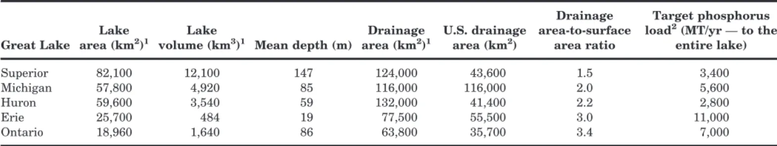
TABLE 1. Morphometric characteristics, drainage basin size, and total targeted annual phosphorus load for each Great Lake.
Great Lake
Lake area (km2)1
Lake
volume (km3)1 Mean depth (m)
Drainage area (km2)1 U.S. drainage area (km2) Drainage area-to-surface area ratio Target phosphorus load2(MT/yr — to the
entire lake) Superior 82,100 12,100 147 124,000 43,600 1.5 3,400 Michigan 57,800 4,920 85 116,000 116,000 2.0 5,600 Huron 59,600 3,540 59 132,000 41,400 2.2 2,800 Erie 25,700 484 19 77,500 55,500 3.0 11,000 Ontario 18,960 1,640 86 63,800 35,700 3.4 7,000
Note: U.S., United States. 1
Encyclopedia Britannica (2019). 2
calibrations, relationships more characteristic to one area, where site density is high, may drive the over-all estimation of the coefficients in the model, and if sites are located too close to one another, measure-ment error may affect the model calibration. In addi-tion, calibration sites are often nested within the basin of downstream sites (in other words upstream of another monitoring site). When this occurs during typical SPARROW calibration, the model-estimated load at each upstream calibration site is replaced with its monitored load to eliminate errors from prop-agating down the stream network and to reduce the correlation across the subbasin error terms (Smith et al. 1997). The resulting downstream load that is estimated using the upstream-measured load is referred to as the “conditioned” predicted load used in model calibration, whereas the load completely simu-lated by the model is referred to as the “uncondi-tioned” predicted load or simply the simulated load. This substitution, however, reduces the magnitude of the errors at the downstream sites, especially when sites have nearby upstream monitored site(s), and can also result in a spatial correlation in the residu-als (Qian et al. 2005). This use of conditioned loads reduces the potential influence of the downstream sites on the coefficients in the SPARROW model and can result in an underestimation of the residuals compared to when the model is used to completely simulate loads throughout the basin (Wellen et al. 2014).
There are significant challenges in developing large scale water-quality models, such as SPARROW models that cover the entire Great Lakes Basin, that include multiple jurisdictions and multiple countries. Because of the different geospatial topologies used to describe stream networks and the different enumera-tion convenenumera-tions used to describe inputs from the var-ious nutrient sources, harmonization (i.e., the process of bringing together data of varying formats, delin-eations, naming conventions and transforming them into one cohesive dataset) of each of the datasets used in the model is required for binational modeling. A precursor to the development of SPARROW models for the entire Great Lakes Basin was the develop-ment of SPARROW models for the Red-Assiniboine River Basin, a region that includes portions of U.S. and Canada, with three states and two provinces (Benoy et al. 2016). Extensive collaboration between agencies in the U.S. and Canada, coordinated by the International Joint Commission, was necessary to create binational harmonized data layers across the entire stream network. Many of the geospatial and numerical techniques used in the Red-Assiniboine River Basin application of SPARROW are applicable elsewhere in other watersheds that straddle the bor-der.
In this paper, we describe the SPARROW P and N models developed for the entire binational Great Lakes Basin and nearby surrounding areas (collec-tively referred to as Midcontinent). These models were developed in a manner which eliminates or at least reduces most of the issues with the original Robertson and Saad (2011) SPARROW models men-tioned above. Additional statistical approaches to those traditionally used to develop SPARROW models are used to reduce the influence of nonuniformly dis-tributed sites and the effects of sites being nested within the basin of other downstream sites. These SPARROW models can be used to describe nutrient sources and transport in the broader Midcontinental region; however, this paper focuses on the Great Lakes. Here, we describe the P and N inputs from the entire Great Lakes Basin, including previously published estimates of interlake inputs and atmo-spheric inputs applied directly to the surface of the lakes. This information enables comparisons and ranking of all contributing areas and enables the importance of the sources throughout the entire area of each of the Great Lakes, or any specified smaller area, such as a specific state/province or specific river basin, to be evaluated. Catchments in the new models are based on a much finer stream network enabling transport to be described over much smaller areas than with the original models.
METHODS
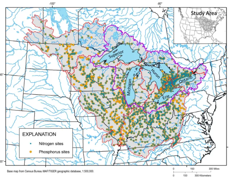
Study Area
Midcontinent SPARROW models were developed for the entire binational Great Lakes Basin and nearby Upper Mississippi River, Ohio River, Red River, and Lake of the Woods Basins (Figure 1). Using information from watersheds near, but outside of, the Great Lakes Basin increased the number of calibration sites which increased the range in model input variability and provided a more accurate repre-sentation of the full range of conditions within the Great Lakes Basin. Land use and land cover in the study area consists primarily of forests in the north-ern and southeastnorth-ern parts and agriculture in the western and central parts. Several major metropoli-tan areas, including Minneapolis, Minnesota, Chi-cago, Illinois, Detroit, Michigan, and Cleveland, Ohio, and Toronto, Ontario, are within this area. The Lau-rentian Great Lakes consist of five lakes linked by relatively short connecting channels. The morphomet-ric characteristics of each lake are given in Table 1. All of the lakes have relatively small drainage
area-to-lake surface area ratios, ranging from 1.5 for Supe-rior to 3.4 for Ontario, and have mean depths ranging from 19 m (Erie) to 147 m (Superior).
SPARROW Model
SPARROW is a spatially referenced watershed model that uses a hybrid mass-balance/statistical approach to simulate the nonconservative transport (i.e., includes losses) of a constituent throughout a study area in relation to statistically significant landscape properties, such as climate, soils, and artificial drainage, and instream/reservoir properties (Smith et al. 1997; Schwarz et al. 2006; Alexander et al. 2008). SPARROW models simulate long-term mean-annual transport (loads, the dependent vari-able in the calibration process) given source inputs and management practices similar to a given base
year (in this case 2002). SPARROW models simu-late long-term mean-annual constituent transport (i.e., loading) that incorporates a range in hydrologi-cal conditions; therefore, they include inputs from both surface-water runoff and groundwater during baseflow and high-flow events. Spatial variability in the environmental setting (described with land-to-water delivery variables) enables variability in the amount of a constituent from each source reaching the stream network. The coefficient reported for each source variable provides an estimate of how much of that source is delivered to streams under the assumption that all spatially variable land-to-water delivery factors are uniformly distributed at average conditions throughout the study area. Part of the constituents that reach the stream is often attenuated or decayed in streams or reservoirs as the constituent travels down the stream network. The amount of a constituent ultimately transported
Study Area
FIGURE 1. Spatial domain of the Midcontinent SPAtially Referenced Regression On Watershed (SPARROW) models, with monitoring sites that were used for model calibration for phosphorus and nitrogen identified.
or delivered to a downstream location incorporates the fraction of the inputs delivered to the stream and the fraction delivered during downstream trans-port, both of which are estimated during calibra-tion.
In SPARROW model development/calibration, a variety of model specifications (regression equations) are evaluated to determine which constituent sources, landscape characteristics, and stream/reservoir decays are statistically significant in controlling constituent transport. In some cases, variables serve as surrogates for other variables that are spatially correlated with the variables specified in the model. For example, although the amount of agricultural land is included as an input source in the N model, it may actually rep-resent N from natural sources, fixation, and other agri-cultural sources that are not included in the model. Variables identified as statistically significant (typi-cally p < 0.05) in explaining the distribution in con-stituent loads are retained, or if source variables are not statistically significant, they are typically com-bined with other sources in a series of model calibra-tions until an acceptable specification is obtained in terms of model fit (root mean square error [RMSE], model-estimated coefficients, variance inflation fac-tors, and residual plots). It is often difficult to com-pletely distinguish the inputs from correlated source variables (such as fertilizer and manure) and this results in large variance inflation factors and rela-tively large confidence limits on their respective coeffi-cients. Highly correlated important land-to-water delivery variables often results in one of the variables being omitted from the model. Coefficients in the mod-els are typically estimated using nonlinear least squares regression (NLLSR; Schwarz et al. 2006). The least squares methodology used to calibrate the model correctly accounts for the enhanced uncertainty caused by collinear variables (Amemiya 1985; Schwarz et al. 2006). If the estimated coefficients associated with collinear variables are statistically significant in the regression, then the implication is that there was a sufficient number of observations to statistically sepa-rate these coefficients from zero.
During calibration, it is optimal to have calibration sites equally distributed throughout the entire study area. Monitoring sites with estimated P and N loads were not evenly distributed over the study area, espe-cially north of Lake Erie (where site density was highest) and north of Lake Superior (where site den-sity was lowest). Therefore, to obtain a more uniform distribution of sites and reduce the effects of mea-surement errors on closely located sites, calibration sites were thinned to only one site from each 12-digit hydrologic unit code (HUC12; Seaber et al. 1987) in the U.S. or HUC12-equivalent sized areas (~100 km2) in Canada. The site with the best estimated load,
based on its coefficient of variation from the modified Beale ratio estimator (BRE) or regression approaches (Cohn 2005; Lee et al. 2016; discussed in the Con-stituent Load Information section), was the site selected from each HUC12. This thinning process did not result in a uniform distribution, but it did reduce dense concentrations in some areas (Figure 1).
During calibration, it is optimal for each monitor-ing site to have similar influence on the determina-tion of coefficients for the variables in the SPARROW model. Because of the way nested sites (a monitoring site located downstream of another monitored site) are typically handled in model calibration, however, the downstream sites tend to have lower residual variance and can result in these sites being underrep-resented in the SPARROW statistical calibration pro-cess. To address for the potential unequal influence of the nested basins during model calibration, a statisti-cal algorithm was developed in which residual weights are computed as being proportional to the fraction of the upstream drainage area that is down-stream of other monitoring sites (the nested area), and these weights are used in a subsequent reestima-tion of the model using weighted-nonlinear least squares regression, WNLLSR (Schwarz et al. 2006, eq. 1.55). To obtain the weights for each site, the SPARROW model is first calibrated with NLLSR using equal weights applied to all sites to obtain an initial estimate of the model residuals. The squared values of the model residuals are then regressed on the fraction of each monitored basin that is down-stream of other monitoring sites (sites with no upstream monitoring sites are assigned a value of 1.0), and if there is a significant relation then the inverse of the predicted values from this regression serve as weights in a subsequent reestimation (recali-bration) of the SPARROW model. The specific equa-tion for determining the weights (wi) is
wi ¼ N 1PNj¼1r2 j r2 i ;
where N is the number of sites and r2
i and r2j are the
residual variances for the i-th and j-th sites, respec-tively. The numerator in the weight equation, given by the average of the residual variances, normalizes the weights so that the variance of the residuals from the WNLLSR approximately equals the residual vari-ance in the unweighted regression. Because the coef-ficient associated with the squared residual and fraction nested area regression relation has a positive sign, this results in a second SPARROW model cali-bration that uses larger, but more proper, residual weights for the load observations associated with sites that have small areas downstream of other
monitoring sites. During this process, the model spec-ification (final variables included in the model and their coefficients) should again be evaluated in an iterative manner. To demonstrate the robustness of the final models, confidence intervals were deter-mined for each coefficient using the standard errors (SEs) from the WNLLSR and the quantile from the standard t distribution.
SPARROW models provide estimations for each stream reach that include incremental (originating in the immediate catchment area) and accumulated (originating in the immediate and all upstream catch-ments) load and yield, volumetrically weighted con-centration, and source-share contributions. In addition, the delivered incremental and accumulated load/yield from any location is described as that part of the load/yield (delivery fraction) ultimately trans-ported downstream to a specific location, in this case each of the Great Lakes, after accounting for down-stream removal/attenuation in down-streams and reser-voirs. Loads and yields (with confidence limits) were simulated for all of the Great Lakes, eight-digit HUCs (HUC8s) in the U.S. and sub-subbasins in Canada, and tributaries with drainage areas > 150 km2 and provided in the Supporting Information to this paper. Because of the nonlinear manner in which the estimated coefficients enter SPARROW models, it was necessary to use bootstrap methods (parametric) to assess uncertainty, which included correcting for potential bias caused by logarithmic retransforma-tions. For a full description of bootstrap methodology, see Schwarz et al. (2006).
Data Used to Calibrate the SPARROW Models
Four types of data are used to “build or calibrate” SPARROW models: stream and reservoir network information to define stream reaches and catchments and to define instream/reservoir decay; long-term mean-annual loads for many sites throughout the study area (dependent variables); information describing all of the main sources of the constituent being modeled (in this case total phosphorus, P, and total nitrogen, N, independent variables); and infor-mation describing variability in the environmental characteristics of the study area that causes statisti-cally significant variability in the land-to-water deliv-ery of the constituent (independent variables). All stream and reservoir information and geographic data used to develop the models are described in detail by Vouk et al. (2018a) and constituent loading data are described by Saad et al. (2018) and briefly described below. Great care was taken to harmonize all data across the U.S.–Canada border, and across state/province borders. As a first step in developing
approaches to create harmonized binational SPAR-ROW models, a modeling team, including scientists from the U.S. and Canada, developed SPARROW P and N models for the Red-Assiniboine River Basin (Jenkinson and Benoy 2015; Benoy et al. 2016).
Stream Network Information. Water flow paths, incremental reaches, and catchments were defined by streams and water bodies in the 1:100,000-scale National Hydrography Dataset Plus Version 2.0 (Moore and Dewald 2016) for the U.S. and a modified version of the Ontario Integrated Hydrology Data Enhanced Watercourse dataset developed by the Ontario Ministry of Natural Resources and Forestry (2012) for Canada (Vouk et al. 2018a). Additional reservoir information was included from the U.S. Army Corps of Engineers National Inventory of Dams dataset for the U.S. (USACE 2016) and CanVec dataset (Centre for Topo-graphic Information 2012) for Canada. Only reser-voirs with surface areas >0.007 km2 were included. Final datasets included ~820,000 catchments, with a median size of 2.5 km2 (mean size of 1.2 km2), with
~265,000 containing reservoirs, compared to ~11,500 catchments, with a median size of ~480 km2, with only 1,045 containing reservoirs in the original Robertson and Saad (2011) models.
Stream length and mean-annual flow velocity were used to estimate the time of travel used to test for nutrient loss due to natural processes in different-sized streams (categorized as small, medium, and large streams). Phosphorus and Nitrogen removal in various-sized streams were examined in the calibra-tion process, but only medium-sized streams (flow rates of 0.28–2.27 m
3
/s; 10–80 cfs) were found to have significant P losses in the final SPARROW P model, and no stream categories had significant N losses in the final SPARROW N model. Reservoir surface area and mean-annual flow were used to compute the inverse of hydraulic loading (flow divided by surface area), which was used to test for P and N removal in reservoirs. Mean-annual flow was obtained from run-off rates reported by McCabe and Wolock (2011) and Wolock and McCabe (2018) for the U.S. and Water Survey of Canada gaging stations data in the Envi-ronment and Climate Change Canada (ECCC) HYDAT database for Canada (Vouk et al. 2018a).
Constituent Load Information. Long-term mean-annual loads representing the 2002 base year were computed for sites having adequate streamflow and water-quality data. Load calculation methods and evaluation criteria are described in detail by Saad et al. (2018) and summarized here. These meth-ods and criteria were based on a study by Saad et al. (2011), who evaluated many of the factors affecting
the accuracy of load estimation. These methods and criteria attempt to balance the SPARROW model need for numerous sites representing the wide range in watershed characteristics that exist throughout the entire study area with the ability to simulate rea-sonably accurate loads. Adequate streamflow required sites to have at least 2 years of complete daily flows collected at or near the monitored location between October 1, 1970 and September 30, 2012, including flow data in 2002 (the base year for the model). Data were compiled from the U.S. Geological Survey (USGS) National Water Information System database (U.S. Geological Survey 2017) for the U.S. and ECCC HYDAT database (ECCC 2016) for Canada. An expansive effort was made to inventory, evaluate, and compile water-quality data from numerous fed-eral, state/provincial, tribe, regional government agencies, and nongovernmental organizations in both U.S. and Canada. Adequate water-quality data required a site to have at least 25 P or N samples during 1970–2012, which minimally overlapped with streamflow data representing that site for 2 years. All water-quality records must be within a predefined proximity to 2002, which depended on the length of the water-quality record. See Saad et al. (2018) for details on the temporal proximity requirements.
For each site, long-term mean-annual P and/or N loads were computed using the Fluxmaster program (Schwarz et al. 2006), which estimates loads using both a regression approach (Cohn 2005) and modified BRE approach (Lee et al. 2016). Both approaches take advantage of measured water quality collected over a range of flow conditions to estimate water quality for days when the site was not monitored, including days with high flows when much of the nutrients is transported. The BRE approach is typi-cally used to compute annual loads; however, in Flux-master, the BRE approach was used to estimate the long-term mean-annual load using eight strata formed by subdividing daily average flows from all years into two classes (delineated by the 80th per-centile of flow) and four seasons. The regression-based approach used a five-variable water-quality model that was a function of flow, seasonality (sine and cosine terms), trend, and an intercept. Both the BRE load and regression-based load detrended to 2002 were computed for each site.
The original SPARROW models (Robertson and Saad 2011) were calibrated with loads computed using only the regression approach, which was later shown to occasionally provide inaccurate and possibly biased loads (Stenback et al. 2011; Richards et al. 2013; Hirsch 2014). To minimize this problem, long-term mean-annual BRE-computed loads computed using the entire period of flow were used whenever there was no trend in the loads because this approach
was shown to have little bias and better at estimating long-term mean-annual loads than most regression approaches (Lee et al. 2016). For sites with no trend in loads, the BRE-computed loads were on average 18% higher than the regression-computed P loads and 8% lower for N loads, which is consistent with that found by Richards et al. (2013). If there was a significant (p < 0.05) trend in load, a mean-annual load detrended to 2002 computed using the regression approach was considered for use in model calibration. Prior to use, all loads were evaluated for accuracy and bias. Load relations with SE > 50% of the mean load estimate were considered unacceptable, which is consistent with the accuracy level used in previous SPARROW studies (Saad et al. 2011), and dropped from consideration. Potential biases in regression-computed loads were calculated as the ratio (R) of BRE load divided by the regression load. For loads having trends, R can deviate from 1.0 even if load estimates have no bias because of the trend in water quality and the proximity of the center of the water-quality record compared to the base year. Therefore, a trend-adjusted acceptable bias range was computed using a trend factor m, where m = exp (trend in load 9 number of years from the midyear of the data-set), in years away from 2002. In staying consistent with a 50% acceptable difference in the SE of the loads, the acceptable range for the ratio was m/ 1.5 < R < m 9 1.5. If R was outside this range, the regression-computed load was considered unaccept-able, and dropped.
Although, much nutrient monitoring has been con-ducted, only a small subset of these sites had suffi-cient data to compute loads using our criteria. After evaluation of 35,000 sites with nutrient data, there were 1,425 sites for which P loads were computed and 1,289 sites for which N loads were computed. Therefore, if the goal of monitoring was to describe nutrient loading, more comprehensive monitoring protocols were needed. Approximately 70% of the loads were computed using the BRE approach. Most of the final load sites easily exceeded the minimum flow and water-quality criteria selection protocols. More than 95% of the sites had at least 10 years of flow record. More than 50% of the P loads had at least 146 water-quality samples covering 25 years or more; 80% had at least 60 samples covering more than 11 years. More than 50% of the N loads had at least 125 water-quality samples covering 26 years or more; 80% had at least 51 samples covering more than 12 years. While there were no criteria explicitly used to identify sites that represent the range in flow and seasonal conditions, the final set of load sites also represented these conditions reasonably well. The ratio of average flow on sampled days to average flow for the full flow record was used to evaluate how well
the range in flow was represented in the monitored loads. Ratios > 1 indicate that samples, on average, represent higher flow conditions and ratios < 1 indi-cate samples represent lower flow conditions. Average and median ratios were close to 1 (the average was 0.99 for P and 1.04 for N and medians for both were 1.0). Seasonal conditions were evaluated by looking at the number of sites with at least three samples in each of the four seasons: 86% of the P sites and 87% of N sites had at least three samples collected in each of the four seasons. Based on these evaluations, the loads were believed to represent the range in flow and seasonal conditions reasonably well.
There was wider range in watershed sizes for sites with loads used in the current model calibration than used in the original models: the 5th percentile was ~45 km2 and 95th percentile was ~36,500 km2 com-pared to a 5th percentile of ~156 km2 and 95th per-centile of ~33,200 km2 for sites used by Robertson and Saad (2011).
Phosphorus and Nitrogen Source Informa-tion. Input to the SPARROW models included data that attempt to describe or quantify all the major sources of P and N. After evaluating a variety of model specifications, the final P model included six P sources: WWTPs, urban and open/barren areas (col-lectively referred to as urban areas), farm fertilizers, manure, agricultural land, and forest/wetland (collec-tively referred to as forested areas). The area of agri-cultural land was used to represent all nonfertilizer and nonmanure sources in agricultural areas, such as natural sources and increased erosion because of agricultural activities. The final N model included five N sources: WWTPs, urban areas, farm fertilizers, manure, and atmospheric deposition. Since there is no general agricultural term in the N model, all increased losses of N in agricultural areas are included in the fertilizer and manure terms. Since there is no atmospheric deposition in the P model, this source would be captured in the other sources. Both models also had direct input from the Missouri River in the U.S. and the Qu’Appelle River in Canada, which contributed P and N from outside the study area. Their inputs were estimated from gaged locations at the study-area boundary. Phosphorus or Nitrogen inputs as point sources, land applied, or as related to land use characteristics for each catchment were estimated for the 2002 base year, or as close to that year as possible. All sources and specified land use characteristics are described in detail by Vouk et al. (2018a) and described briefly here.
WWTP effluent data (flow and P and N concentra-tion data) were obtained from the U.S. Environmen-tal Protection Agency Permit Compliance System database supplemented with additional data obtained
directly from the states of Wisconsin and Minnesota for the U.S. and Ontario Clean Water Agency and Ministry of the Environment and Climate Change for Ontario. Phosphorus and Nitrogen effluent loads were then computed for each WWTP with or without concentration data (concentrations for sites without measurements were estimated based on typical pollu-tant concentrations for the magnitude of flow for the facility) using methods described by McMahon et al. (2007), Hoos et al. (2008), and Vouk et al. (2018a). Manitoba and Saskatchewan effluent loads were calcu-lated based on population in the catchment and an export per capita rate based on data obtained from Manitoba Conservation and Water Stewardship, and Saskatchewan Ministry of Environment and the Sas-katchewan Water Security Agency (Vouk et al. 2018a). Fertilizer and manure inputs to each catchment were estimated from total county applications in the U.S. or sub-subbasins in Canada and the amount of agricultural land in each county or sub-subbasin. Inorganic farm fertilizer (referred to as fertilizer) inputs in the U.S. were based on 2002 county-level estimates from Ruddy et al. (2006) and in Canada were based on 2001 Census of Agriculture (AAFC 2002, 2007) data by census division and census con-solidated subdivision. Manure inputs were estimated from 2002 county livestock head counts from the Cen-sus of Agriculture (NASS 2004; Mueller and Gron-berg 2013) for the U.S., and by sub-subbasin estimates for 2001 from the Interpolated Census of Agriculture (AAFC 2001) for Canada. Phosphorus and Nitrogen manure coefficients for each animal type were obtained from Ruddy et al. (2006).
Land use-related inputs (export from a general land type) were based on the amount of the catch-ment (in km2) in each general land type (i.e., urban, agriculture, and forested) represented in the 2001 National Land Cover Data (Homer et al. 2007) for the U.S. and the Natural Resources Canada Geobase land cover-data circa 2002 (Centre for Topographic Information 2009) for Canada. Export coefficients for each land type were estimated in the SPARROW cali-bration process.
Total atmospheric deposition of N in 2002 onto each catchment was estimated from Congestion Mitigation and Air Quality Improvement (CMAQ) Program depo-sition rates (Schwede et al. 2009; Hong et al. 2011; USEPA 2018b) and the area of the catchment.
Environmental Setting Variables. Statistical methods, similar to those used for determining which P and N sources to include in the models, were used to identify which characteristics were important in explaining variability in P and N delivery to streams. Many characteristics thought to affect nutrient deliv-ery to streams were examined in determining which
statistically significant land-to-water delivery factors to include in the models. Environmental setting data were summarized into an average value for each catchment (e.g., average air temperature) or percent-age of the catchment with a specific characteristic (e.g., percent clay content).
Environmental setting variables found to signifi-cantly influence land-to-water delivery of P were air temperature and percent soil clay content. For the N model, significant variables included air temperature, catchment runoff, and percent of the catchment underlain with tile drains. Mean air temperatures, representing the 1971–2000 average, were obtained from the PRISM database (PRISM Climate Group 2009) for the U.S. and from the Canadian Forest Ser-vice (McKenney et al. 2006) for Canada. The average percent clay in the soil was estimated from data in the U.S. Department of Agriculture STATSGO data-base using methods described by Wolock (1997) for the U.S. and estimated from data from Soil Land-scape of Canada version 2.2 (AAFC 1996) for Canada; areas of missing data in Canada were estimated with assistance from the Agriculture and Agri-Food Canada. Mean-annual runoff for 1971–2000 was esti-mated from annual runoff values from the Wolock and McCabe (1999, 2018) water balance model for the U.S. This model was also used to estimate mean-annual runoff from 1971 to 2000 from Canadian catchments using air temperature from the Canadian Forest Service (McKenney et al. 2006) and precipita-tion from the Canadian Precipitation Analysis (National High Impact Weather Laboratory 2014). Percent of the catchment with tile drains in the U.S. was based on early 1990s tile drain information com-piled by Nakagaki et al. (2016) following the methods described by Sugg (2007). Percent of the catchment with tile drains in Ontario catchments was obtained from Ontario Ministry of Agriculture Food and Rural Affairs (2015) data, and in Manitoba catchments from Sustainable Development (Vouk et al. 2018a). Because of the aridity of Saskatchewan, tile drains were assumed to be absent in this province. All envi-ronmental setting data used in the models are described in detail by Vouk et al. (2018a).
Atmospheric Deposition on the Lakes and Interlake Transport. Total atmospheric deposition of N onto each lake was computed from their surface areas and total deposition rates for 2002 from the CMAQ Program (Schwede et al. 2009; Hong et al. 2011; USEPA 2018b). Total deposition of P onto each lake for 2002 was computed by linearly detrending annual depositions to each lake published by Dolan and Chapra (2012) to 2002. Linearly detrending annual data to 2002 was done by regressing the annual deposition rates on years and determining the
deposition value for 2002. Contributions from the adjacent upstream lake(s) were estimated from annual interlake transport estimated by Dolan and Chapra (2012), who estimated interlake transfer of P from measured flow between the lakes and observed in lake concentrations. Interlake P input in 2002 was estimated by linearly detrending the annual inputs. Interlake N inputs were estimated from the interlake P input and the ratio of total N to total P measured during spring in each lake from Dove and Chapra (2015) for the 2–3 years centered on 2002. Total N was based only on the sum of nitrite plus nitrate and ammonia. Organic N was not included because it was not measured during routine monitoring; therefore, the interlake transfer of N is biased low.
RESULTS
Calibration of SPARROW Models
Preliminary SPARROW P and N models were first developed using all load sites that met the defined accuracy criteria (the typical approach used in devel-oping SPARROW models), which identified an initial list of potential source, land-to-water delivery, and instream decay variables. The initial variables included in this traditional model-development approach ("all data") are given in Table 2, which pro-vides an example of the full calibration process for the P model. Next, the sites were thinned down to one site per HUC12-sized area, and the variables included in the model were reevaluated. This thin-ning process reduced the number of load sites from 1,425 to 1,197 for P and from 1,289 to 1,101 for N (the final, thinned sites used for model development are shown in Figure 1). This step dropped basin slope from the model, and it affected the magnitude of a few coefficients for the variables, especially the WWTP coefficients (“thinned” in Table 2). For the final calibration step, the model residuals were exam-ined to see if they were significantly related to the fraction of the basin that was nested. The residuals were significantly related to the fraction of the basin that was nested (p < 1.0 e 23); therefore, the weight of each thinned-calibration site was adjusted based on the fraction of its drainage area that was down-stream of other monitoring sites and the model was reevaluated. During typical SPARROW calibrations, all sites are equally weighted. The weights applied to the sites in nested-weighting calibration ranged by about a factor of 10 for P and a factor of 5 for N, with sites having small areas downstream of other moni-toring sites having larger weights. Model specification
in the last two steps was done in an iterative man-ner, until the final variables were chosen.
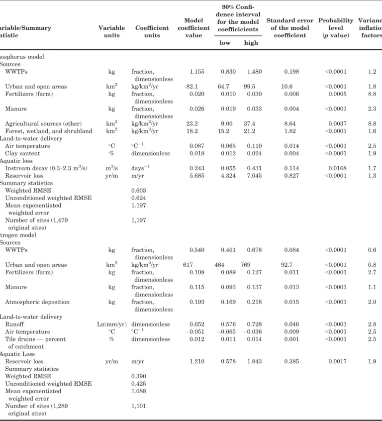
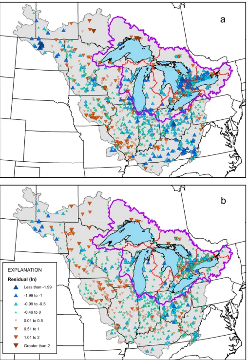
The final SPARROW P model was a function of: six P sources (WWTPs, urban land, farm fertilizers, manure, agricultural land, and forested land); two land-to-water delivery factors (air temperature and percent clay content); nutrient removal in medium-sized streams; and deposition in reservoirs (Tables 2 and 3). The coefficients for all sources and factors were highly significant (p < 0.02), indicating that each source, land-to-water delivery factor, and instream/reservoir factor was important in describing the distribution in measured loads. The coefficients were also robust (see the 90% confidence intervals for the coefficients in Table 3). This P model had a condi-tioned RMSE of 0.603 (based on comparisons of mea-sured and conditioned predicted loads in natural logarithmic units). Based on full model predictions (based on unconditioned simulated loads), the uncondi-tioned RMSE was 0.624. The distribution of the uncon-ditioned residuals is shown in Figure 2a. A few regional biases in model unconditioned simulated loads occurred but were mostly outside of the Great Lakes Basin (overestimations in the extreme the northwest and southeast and underestimations in the southwest); however, areas north of the Great Lakes, where few calibration sites exist, were also underestimated.
In SPARROW models, the export of each source from a catchment, except point sources, is usually modified by land-to-water delivery factors. The values
of the coefficients associated with each source (Table 3) describe the average effect of the land-to-water delivery factors, but spatial variability in these factors enable variability in transport of the sources to streams across the study area. WWTP effluent is directly added to the stream network. The coefficient for WWTP (1.155) being >1.0 suggests that either WWTP input may have been underestimated, or more likely that this variable also incorporates the effects of other sources, such as commercial and industrial point sources and combined sewer overflows. The cali-brated model indicates that urban areas on average contribute ~82 kg/km2/yr in addition to contributions from WWTPs. There were three agricultural sources, namely fertilizers, manure, and a general agricul-tural area source. The fertilizer and manure coeffi-cients suggest that ~2.0% of the input from farm fertilizers reach streams compared to ~2.6% for man-ure (coefficients = 0.020 and 0.026, respectively), although these percentages were not statistically dif-ferent. The calibrated model indicates that agricul-tural areas contribute an additional ~23 kg/km2/yr to that from fertilizers and manure, which represents general losses from agricultural areas, such as natu-ral sources and increased losses caused by agricul-tural activity. On average, forest, wetland, and shrubland areas are estimated to contribute ~18 kg/ km2/yr. The P model did not include atmospheric deposition; therefore, this source would be included in the other defined sources.
TABLE 2. Summary of model development for the phosphorus SPARROW model.
Variable/Summary statistic Variable units
Model coefficients
All data Thinned data set
Thinned and adjusted for nesting (final model1) Sources
Wastewater treatment plants (WWTPs) kg 1.152 1.020 1.155
Urban and open areas km2 82.71 90.01 82.08
Fertilizers (farm) kg 0.018 0.019 0.020
Manure kg 0.022 0.026 0.026
Agricultural sources (other) km2 40.39 28.16 23.21
Forest, wetland, and shrubland km2 17.52 17.72 18.20
Land-to-water delivery
Air temperature °C 0.083 0.083 0.087
Clay content % 0.019 0.019 0.018
Basin slope degrees 0.049 NI NI
Aquatic loss
Instream decay (0.3–2.3 m
3/s) m3/s 0.262 0.328 0.243
Reservoir loss yr/m 5.104 4.867 5.685
Summary statistics
Unconditioned RMSE 0.6542 0.654 0.6503
Number of sites 1,425 1,197 1,197
Note: Calibration incorporated adjustments for the high density of sites in specific areas (thinned) and the amount of the upstream water-shed downstream of other calibration sites (nested area) (NI, not statistically significant in model; therefore, not included in the model). 1
Full final model results are provided in Table 3.
2Root mean square error (RMSE) computed only for the thinned 1,197 sites. 3Not adjusted for different weighting applied to the sites.
Reckhow et al. (1980) and Beaulac and Reckhow (1982) conducted a literature search of nutrient export rates for selected land uses and found P export of 2–82 kg/km2 (median of 22 kg/km2) from forested
areas, 19–623 kg/km
2
(median of 108 kg/km2) from urban areas, and 10–1,860 kg/km2 (medians of
225 kg/km2from row crops and 100 kg/km2from pas-ture) from agricultural areas. Our estimated yields
TABLE 3. Summary of SPARROW model calibration results.
Variable/Summary statistic Variable units Coefficient units Model coefficient value 90% Confi-dence interval
for the model coefficicients Standard error of the model coefficient Probability level (p value) Variance inflation factors low high Phosphorus model Sources WWTPs kg fraction, dimensionless 1.155 0.830 1.480 0.198 <0.0001 1.2 Urban and open areas km2 kg/km2/yr 82.1 64.7 99.5 10.6 <0.0001 1.8 Fertilizers (farm) kg fraction,
dimensionless
0.020 0.010 0.030 0.006 0.0005 8.8
Manure kg fraction,
dimensionless
0.026 0.019 0.033 0.004 <0.0001 2.3 Agricultural sources (other) km2 kg/km2/yr 23.2 9.00 37.4 8.64 0.0037 8.8 Forest, wetland, and shrubland km2 kg/km2/yr 18.2 15.2 21.2 1.82 <0.0001 1.6 Land-to-water delivery
Air temperature °C °C 1 0.087 0.065 0.110 0.014 <0.0001 2.5 Clay content % dimensionless 0.018 0.012 0.024 0.004 <0.0001 1.9 Aquatic loss
Instream decay (0.3–2.3 m
3/s) m3/s days 1 0.243 0.055 0.431 0.114 0.0168 1.7 Reservoir loss yr/m m/yr 5.685 4.324 7.045 0.827 <0.0001 1.3 Summary statistics
Weighted RMSE 0.603
Unconditioned weighted RMSE 0.624 Mean exponentiated weighted error 1.197 Number of sites (1,479 original sites) 1,197 Nitrogen model Sources WWTPs kg fraction, dimensionless 0.540 0.401 0.678 0.084 <0.0001 0.6 Urban and open areas km2 kg/km2/yr 617 464 769 92.7 <0.0001 0.8 Fertilizers (farm) kg fraction,
dimensionless
0.108 0.089 0.127 0.011 <0.0001 2.7
Manure kg fraction,
dimensionless
0.115 0.093 0.137 0.013 <0.0001 1.1 Atmospheric deposition kg fraction,
dimensionless
0.193 0.169 0.218 0.015 <0.0001 2.0 Land-to-water delivery
Runoff Ln(mm/yr) dimensionless 0.652 0.576 0.728 0.046 <0.0001 2.8 Air temperature °C °C 1 0.051 0.065 0.036 0.009 <0.0001 2.5 Tile drains— percent
of catchment
% dimensionless 0.012 0.011 0.014 0.001 <0.0001 2.5 Aquatic Loss
Reservoir loss yr/m m/yr 1.210 0.578 1.843 0.385 0.0017 1.9
Summary statistics
Weighted RMSE 0.390
Unconditioned weighted RMSE 0.425 Mean exponentiated weighted error 1.088 Number of sites (1,289 original sites) 1,101
for forested, urban, and agricultural areas are in the range of those published. Our export rates from urban areas did not include WWTP effluent and from agricultural areas do not include export from fertiliz-ers and manure, which likely resulted in our esti-mated rates being on the low end of those published.
Based on the sign of the land-to-water delivery coefficients (positive values reflect enhanced deliv-ery), P yields were higher in areas with higher air temperatures and higher clay content. Streams were subdivided into three sizes based on their average
with mean-annual streamflow (<0.3 m3/s; 0.3–2.3 m3/s; and >2.3 m3/s). Instream losses were only significant in medium-sized streams (0.3–2.3 m
3
/s; 8–80 ft
3
/s), and not significant in small and large streams. The optimum range of streams with instream losses was found by iteratively changing the ranges to minimize
p values during model calibration. P removal in
reser-voirs was also significant.
A similar approach to that used for P was used to develop the final SPARROW N model. The final N model had: five N sources (WWTPs, urban areas,
# * # * # * # * # * # * # * # * # * # * # * # * # * # * # * # * # * # * # * # * # * # * # * # * # * # * # * # * # * # * # * # * # * # * # * # * # * # * # * # * # * # * # * # * # * # * # * # * # * # * # * # * # * # * # * # * # * # * # * # * # * # * # * # * # * # * # * # * # * # * # * # * # * # * # * # * # * # * # * # * # * # * # * # * # * # * # * # * # * # * # * # * # * # * # * # * # * # * # * # * # * # * # * # * # * # * # * # * # * # * # * # * # * # * # * # * # * # * # * # * # * # * # * # * # * # * # * # * # * # * # * # * # * # * # * # * # * # * # * # * # * # * # * # * # * # * # * # * # * # * # * # * # * # * # * # * # * # * # * # * # * # * # * # * # * # * #* # * # * # * # * # * # * # * # * # * # * # * # * # * # * # * # * #* # * # * # * # * # * # * # * # * # * # * # * # * # * # * # * # * # * # * # * # * # * # * # * # * # * # * # * # * # * # * # * # * # * # * # * # * # * # * # * # * # * # * # * # * # * # * # * # * # * # * # * # * # * # * # * #* # * # * # * # * # * # * # * # * # * # * # * # * # * # * # * # * # * # * # * # * # * # * # * # * # * # * # * # * # * # * # * # * # * # * # * # * # * # * # * # * # * # * # * # * # * # * # * # * # * # * # * # * # * # * # * # * # * # * # * # * # * # * # * # * # * # * # * # * # * # * # * # * # * # * # * # * # * # * # * # * # * # * # * # * # * # * # * # * # * # * # * # * # * # * # * # * # * # * # * # * # * # * # * # * # * # * # * # * # * # * # * # * # * # * # * # * # * # * # * # * # * # * # * # * # * # * # * # * # * # * # * # * # * # * # * # * # * # * # * #* # * # * # * # * # * # * # * # * # * # * # * # * # * # * # * # * # * # * # * # * # * # * # * # * # * # * # * # * # * # * # * # * # * # * # * # * # * # * # * # * # * # * # * # * # * # * # * #* # * # * # * # * # * # * # * # * # * # * # * # * # * # * # * # * # * # * # * # * # * # * # * # * # * #* # * # * # * # * # * # * # * # * # * # * # * # * # * # * # * # * # * # * # * # * # * # * # * # * # * # * # * # * # * # * # * # * # * # * # * # * # * # * # * # * # * # * # * # * # * # * # * # * #* # * # * # * # * # * # * # * # * # * # * # * # * # * # * # * # * # * # * # * # * # * # * # * # * # * # * # * # * # * # * # * # * # * #* #* # * # * # * # * # * # * # * # * # * # * # * # * # * # * # * # * # * # * # * # * # * # * # * # * # * # * # * # * # * # * # * # * # * # * #* # * # * # * # * # * # * # * # * # * # * # * # * # * # * # * # * # * # * # * # * # * # * # * # * # * # * # * # * # * # * # * # * # * # * # * # * # * # * # * # * # * # * # * # * # * # * # * # * # * # * # * # * # * # * # * # * # * # * # * # * # * # * # * # * # * # * # * # * # * # * # * # * # * # * # * # * # * # * # * # * # * # * # * # * # *#* # * # * # * # * # * # * # * # * # * # * # * # * # * # * # * # * # * # * # * # * # * # * # * # * # * # * # * # * # * # * # * # * # * # * # * # * # * # * # * # * # * # * # * # * # * # * # * # * # * # * # * # * # * # * # * # * # * # * # * # * # * # * # * # * # * # * # * # * # * # * # * # * #* # * # * # * # * # * # * # * # * # * # * # * # * # * # * # * # * # * # * # * # * # * # * #* # * # * # * # * # * # * # * # * # * # * # * # *#* # * # * # * # * # * # * # * # * # * # * # * # * # * # * # * # * # * # * # * # * # * # *#* # * # * # * # * # * # * # * # * # * # * #* # * # * # * # * # * # * # * # * # * # * # * # * # * # * # * # * # * # * # * # * # * # * # * # * # * # * # * # * # * # * # * # * # * # * # * # * # * # * # * # * # * # * # * # * # * # * # * # * # * # * # * # * # * # * # * # * # * # * # * # * #* # * # * # * # * # * # * # * # * # * #* # * # * # * # * # * # * # * # * # * # *#* # * # * # * # * # * # * # * # * # * # * # * # * # * # * # * # * # * # * # * # * # * # * # * # * # * # * # * # * # * # * # * # * # * # * # * # * # * #*#* # * # * # * # * #* # * # * # * # * # * # * # * # * # * # * # * # * # * # * # * # * # * # * # * # * # * # * # * # * # * # * # * #* # * # * # * # * # * # * # * # * # * # * # * # * # * # * # * # * # * # * # * # * # * # * # * # * # * # * # * # * # * # * # * # * # * # * # * # * # * # * # * # * # * # * # * # * # * # * # * # * # * # * # * # * # * # * # * # * # * # * # * # * # * # * # * # * # * # * # * # * # * # * # * # * # * # * # * # * # * # * # * # * # * # * # * # * # * # * # * #* # * # * # * # *#* #* # * # * # * # * # * # * # * # * # * # * # * # * # * # * # * # * # * # * # * # * # * # * # * # *#* # * # * # * # * # * #* # * # * # * # * # * # * # * # * # * # * # * # * # * # * # * # * # * # * # * # * # * # * # * # * # * # * # * # * # * # * # * # * # * # * # * # * # *#* # * # * # * # * # * # * # * # * # * # * # * # * # * # * # * # * # * # * # * #* # * # * # * # * # * #* # * # * # * # * # * # * # * # * # * # * # * # * # * # * # * # * # * # * # * # * # * # * # * # * #* # * # * # * #* # * # * # * # * # * # * # * # * # * # * # * # * # * # * # * # * #* # * # * # * # *#* # * # * # * # * # * # * # * # * # * # * # * # * # * # * # * # * # * # * # * # * # * # * # * # * # * # * # * # * # * # * # * # * # * # * # * # * # * # * # * # * # * # * # * # * # * # * # * # * # * # * # * # * # * # * # * # * # * # * # * # * # * # * # * # * # * # * # * # * # * # * # * # * # * # * # * # * # * # * # * # * # * # * # * # * # * # * # * # * # * # * # * # * # * # * # * # * # * # * # * # * # * # * # * # * # * # * # * # * # * # * # * #* # * # * # * # * # * # * # * # * # * # * # * # * # * # * # * # * # * # * # * # * # * # * # * # * # * # * # * # * # * # * # * # * # * # * # * #* # * # * # * # * # * # * # * # * # * # * # * # * # * # * # * # * # * # * # * # * # * # * # * # * # * # * # * # * # * # * # * # * # * # * # * # * # * # * # * # * # * # * # * # * # * # * # * # * # * #* # * # * # * # * # * # * # * # * # * # * # * # * # * # * # * # * # * # * # * # * # * # * # * # * # * # * # * # * # * # * # * # * # * # * # * # * # * # * # * # * # * # * # * # * # * # * # * # * # * # * # * # * # * # * # * # * # * # * # * # * # * # * # * # * # * # * # * # * # * # * # * # * # * # * # * # * #* # * # * # * # * # * # * # * # * # * # * # * # * # * # * # * # * # * # * # * # * #* # * # * # * # * # * # * # * # * # * # * # * # * # * # * # * # * # * # * # * # * # * # * # * # * # * # * # * # * # * #* # * # * # * # * # * # * # * # * # * # * # * # * # * #* # * # * # * # * # * # * # * # * # * # * # * # * # * # * # * # * # * # * # * # * # * # * # * # * # * # * # * # * # * # * # * # * # * # * # * # * # * # * # * # * # * # * # * # * # * # * # * # * # * # * # * # * # * # * # * # * # * # * # * # * # * # * # * # * # * # * #* # * # * # * # * # * # * # * # * # * # * # * # * # * # * # * # * # * # * # * # * # * # * # * # * # * # * # * # * # * # * # * # * # * # * # * # * # * # * # * # * # * # * # * # * # * # * #* # * # * # * # * # * # * # * # * # * # * # * # * # * # * # * # * # * # * # * # * # * # * # * # * # * # * # * # * # * # * # * # * # * # * # * # * # * # * # * # * # * # * # * # * #* # * # * # * # * # * # * # * # * # * # * # * # * # * # * # * # * # * # * # * # * # * # * # * # * # * # * # * # * # * # * # * # * # * # * # * # * # * # * # * #* # * # * # * #* # * # * # * # * # * # * # * # * # * # * # * # * # * # * # * # * # * # * # * # * # * # * # * # * # * # * # * # * # * # * # * # * # * # * # * # * # * # * # * # * # * # * # * # * # * # * # * # * # * #* # * # * # * # * # * # * # * #* # * # * # * # * # * # * # * # * # * # * # * # * # * # * # * # * # * # * # * # * # * # * # * # * # * # * # * # * # * # * # * # * # * # * # * # * # * # * # * # * # * # * # * #* # * # * # * # * # * # * # * # * # * # * # * # * # * # * # * # * # * # * # * # * # * # * # * # * # * # * # * # * # * # *#* # * # * # * # * # * # * # * # * # * # * # * # * # * # * # * # * # * # * # * # * # * # * # * # * # * # * # * # * # * # * # * # * # * # * # * # * # * #* # * # * # * # * # * # * # * # * # * # * # * # * # * # * # * # * # * # * #* # * # * # * # * # * # * # * # * # * # * # * # * # * # * # * # * # * # * # * # * # * # * # * # * #* # * # * # * # * # * # * # * # * # * # * # * # * # * # * # * # * # * # * # * # * # * # * # * # * # * # * # * # * # * # * # * # * # * # * # * #* # * # * # * # * # * # * # * # * # * # * # * # * # * # * # * # * # * # * # * # * # * # * # * # * # * # * # * # * # * # *#* # * # * # * # * # * # * # * # * # * # * # * # * # * # * # * # * # * # * # * # * # * # * # * # * # * # * # * # * # * # * # *#* # * # * # * # * # * # * # * # * # * # * # * # * # * # * # * # * # * # * # * # * # * # * # * # * # * # * # * # * # * # * # * # * # * # * # *#* # * # * # * # * # * # * # * # * # * # * # * # * # * # * # * # * # * # * # * # * # * # * # * # * # * # * # * # * # * # * # * # * # * # * # * # * # * # * # * # * # * # * # * # * # * # * # * # * # * # * # * # * # * # * # * # * # * # * # * # * # * # * # * # * # * # * # * # * # * # * # * #* # * # * # * # * # * # * # * # * #* # * # * # * # * # * # * # * # * # * # * # * # * # * # *#* # * # * # * # * # * # * # * # * # * # * # * # * # * # * #* # * # * # * # * # * # * # * # * # * # * # * # * # * # * # * # * # * # * # * # * # * # * # * # * # * # * # * # * # * # * # * # * # * # * # * # * # * # * # * # * # * # * # * # * # * # * # * # * # * # * # * # * # * # * # *#* # * # * # * # * # * # * # * # * # * # * # * # * # * # * # * # * # * # * # * # * # * # * # * # * # * # * # * # * # * # * # * # * # * # * # * # * # * # * # * # * # * # * EXPLANATION Residual (ln) # * Less than -1.99 # * -1.99 to -1 # * -0.99 to -0.5 # * -0.49 to 0 # * 0.01 to 0.5 # * 0.51 to 1 # * 1.01 to 2 # * Greater than 2
a
b
FIGURE 2. Predictability of the Midcontinent (a) phosphorus and (b) nitrogen SPARROW models. All residuals are in natural logarithmic units. All major basins are delineated.
farm fertilizers, manure, and atmospheric deposition); three land-to-water delivery factors (runoff, air tem-perature, and percent of the catchment underlain by tile drains); and one factor describing removal in reservoirs (Table 3). Nitrogen from general agricul-tural activities was not found to be significant; there-fore, it would be included in the fertilizer and manure terms. N losses in different-sized streams were examined but were insignificant. The residuals were significantly related to the fraction of the basin that was nested (p < 1.4 e 12); therefore, the weight of each thinned-calibration site was adjusted based on the fraction of its drainage area that was down-stream of other monitoring sites and the model was reevaluated. A significant coefficient describing N losses in medium-sized streams was initially found when all monitoring sites were included, but this coefficient was insignificant when the load data were adjusted for upstream nesting; therefore, instream decay was not included in the final model (discussed later). Coefficients for all variables in the final N model were highly significant (p < 0.002) indicating that each source, land-to-water delivery factor, and reservoir factor was important in describing the dis-tribution in measured N loads. The coefficients were robust (see the 90% confidence intervals in Table 3). This model had a conditioned RMSE of 0.390, and an unconditioned RMSE of 0.425. The distribution of unconditioned residuals is shown in Figure 2b. The only consistent regional biases in unconditioned loads were mostly outside of the Great Lakes Basin (over-estimated in the far northwest).
Source coefficients in the N model indicate that ~54% of the estimated N input from WWTPs, ~11% of farm fertilizers, ~12% of manure, and ~20% of the atmospheric deposition reach the stream network (Table 3). Relatively more of the agricultural N sources (11%–12%) were transported to streams than the agricultural P sources (2%–3%). In addi-tion to effluent from WWTPs, urban areas con-tribute ~616 kg/km2/yr. The WWTP coefficient (0.54) being <1.0 suggests that our WWTP input may have been overestimated. This is not too surprising given that most N inputs from WWTPs were based on typ-ical pollutant concentrations. Additional inputs from agricultural and forested lands were not significant in the N model. Inputs from fixation and other agri-cultural losses are likely to be included with other sources that they may be correlated, such as fertiliz-ers and manure. Losses from forested areas are likely to be included with the atmospheric deposi-tion source. Based on the signs of the land-to-water delivery coefficients, N yields should be higher in areas with higher runoff, cooler air temperatures, and more tile drains. Removal/deposition in reser-voirs was also significant in the model.
Delivered Incremental Nutrient Yields
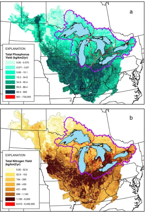
Delivered incremental P and N yields (load per unit catchment area delivered to a specified down-stream target, such as the Great Lakes) from each catchment are shown in Figure 3. Delivered incre-mental yields are mediated by the amount and type of nutrients input to the catchment and by land-to-water delivery, stream, and reservoir factors affect-ing their transport. Highest delivered yields were from catchments with WWTPs, such as Detroit, Michigan, and Chicago, Illinois; however, lower but still relatively high-delivered P yields (>88 kg/km2/ yr) and N yields (>1,140 kg/km2/yr) were from catchments in extensive agricultural areas. Within the Great Lakes Basin, highest P and N yields were primarily around Erie and the southeast shore of Huron and lowest north of Superior. The main dif-ferences in geographic patterns of P and N yields can be explained by differences in agricultural source distributions, with higher P yields from areas dominated by animal agriculture. Accumu-lated P and N loads and yields representing the 2002 base year, with confidence intervals, for each Great Lake, HUC8/sub-subbasin, and tribu-taries > 150 km2 are provided in the Supporting Information. It should be noted that these loads/ yields were not adjusted for the prediction errors shown in Figure 2, that is, they are the noncondi-tioned loads and yields.
Total Phosphorus and Nitrogen Delivery to the Great Lakes
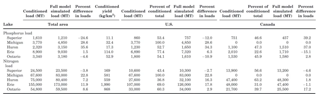
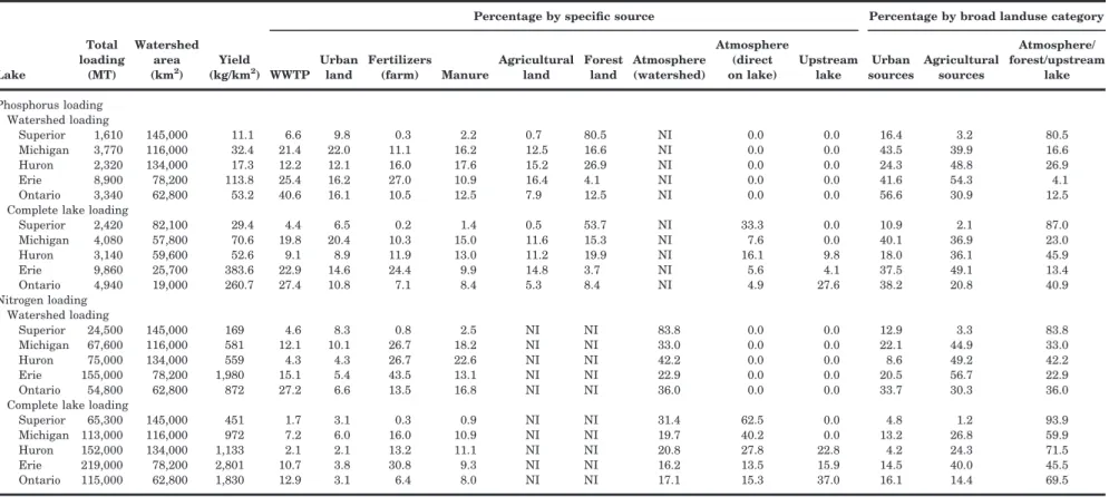
To reduce the effects of prediction errors from the SPARROW models (Figure 2) when estimating the total loads delivered to each Great Lake, model results were used only to simulate loads from unmonitored areas and measured loads were used wherever they were available. This combination of measured and modeled loads is referred to as the “total conditioned” load. The total conditioned P load-ing from the watershed ranged from 1,610 MT/yr (metric tonnes per year) into Superior to 8,900 MT/ yr into Erie (Table 4 and Figure 4a). The percent of the total conditioned load obtained from monitored sites varied among lakes depending on the number and location of the monitoring sites. Contributions of P from Canada ranged from 46%–47% for Superior, Huron, and Ontario, to 23% for Erie, to 0% for Michigan. Full SPARROW-simulated P loads for each lake ranged from being 25% lower to 36% higher than the conditioned loads. The total condi-tioned N loading ranged from 24,500 MT/yr (Supe-rior) to 155,000 MT/yr (Erie; Table 4 and Figure 4b).
Contributions of N from Canada ranged from 56– 63% for Superior and Huron, to 31%–40% for Erie and Ontario, to 0% for Michigan. Full SPARROW-simulated N loads to each lake ranged from being 4% lower to 23% higher than the total conditioned loads.
Annual P yields from the watershed ranged from 11.1 kg/km2 (Superior) to 114 kg/km2 (Erie) and annual N yields ranged from 169 kg/km2 (Superior) to
1,990 kg/km2(Erie; Table 4). Phosphorus and Nitrogen yields from the Erie watershed were much higher than
from other lake watersheds, which coincide with it hav-ing the highest percentage of agriculture in its water-shed. Yields were second highest from the Ontario watershed, followed by Michigan, Huron, and Superior. After including P and N from nontributary sources (interlake transfer and direct atmospheric deposition on the lakes), total annual P loading was 2,420 MT to Superior, 4,080 MT to Michigan, 3,140 MT to Huron, 9,860 MT to Erie, and 4,940 MT to Ontario (Figure 4 and Table 5). All loads are below the targets estab-lished by the GLWQA (Table 1). After including N
TABLE 4. Total annual watershed load (conditioned and fully simulated with the model), in MT to each Great Lakes, total and by country. Lake Conditioned load (MT) Full model simulated load (MT) Percent difference in loads Conditioned yield (kg/km2) Conditioned load (MT) Percent of conditioned total Full model simulated load (MT) Percent difference in loads Conditioned load (MT) Percent of conditioned total Full model simulated load (MT) Percent difference in loads
Total area U.S. Canada
Phosphorus load Superior 1,610 1,210 24.6 11.1 860 53.4 757 12.0 751 46.6 457 39.2 Michigan 3,770 4,850 28.6 32.4 3,770 100.0 4,850 28.6 0 0.0 0 0.0 Huron 2,320 3,150 35.6 17.3 1,230 52.7 1,650 34.3 1,100 47.3 1,510 37.0 Erie 8,900 9,030 1.5 114.0 6,890 77.4 7,320 6.3 2,010 22.6 1,710 15.1 Ontario 3,340 3,180 4.6 52.9 1,800 54.1 1,610 10.9 1,530 45.9 1,580 2.8 Nitrogen load Superior 24,500 23,500 3.8 169 10,600 43.4 10,300 2.7 13,900 56.6 13,200 4.6 Michigan 67,600 83,000 22.8 581 67,600 100.0 83,000 22.8 0 0.0 0 0.0 Huron 75,000 80,400 7.2 559 27,600 36.8 32,100 16.3 47,400 63.2 48,300 1.8 Erie 155,000 173,000 11.9 1,990 107,000 69.0 126,000 17.8 48,000 31.0 47,400 1.1 Ontario 54,800 59,500 8.6 868 33,000 60.3 34,000 2.9 21,700 39.7 25,500 17.2
Note: Conditioned loads are estimated with measured loads and simulated loads from SPARROW for ungaged areas.
OF THE A MERICAN W ATER R ESOURCES A SSOCIATION JAWRA 15 P HOSPH ORUS AND N ITROG EN T RANSPO RT IN THE B INATIONA L G REAT L AKES B ASIN E STIMAT ED U SING SPARROW W ATERSHE D M ODELS
from nontributary sources, total annual N loading was 65,300 MT to Superior, 113,000 MT to Michigan, 152,000 MT to Huron, 219,000 MT to Erie, and 115,000 MT to Ontario.
Sources of Phosphorus and Nitrogen to the Great Lakes
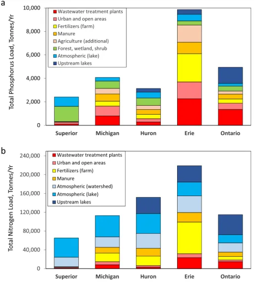
Sources of P in the SPARROW model included inputs from WWTPs, urban land, farm fertilizers, manure, other agricultural sources, and forested land. The percentage of the total P load delivered to each lake originating from each source is shown in Figure 4a and given in Table 5, along with a break-down into broad land use categories: urban, agricul-ture, and forest sources. Each lake had a different ranking in the relative importance of individual P sources. The largest broad land use source was forest sources for Superior, urban sources for Michigan and
Ontario, and agricultural sources for Huron and Erie. The relative importance of each agricultural source is shown for each lake in Figure 4. In general, manure was the largest agricultural P source for all lakes, except Erie that was dominated by fertilizers (Table 5).
The importance of P from WWTPs and other urban sources varied from 16%–24% (Superior and Huron), 42%–44% (Michigan and Erie), to 57% (Ontario) of the watershed loading (Table 5; Figure 4a). This is a decrease in importance compared to that estimated by Robertson and Saad (2011) (discussed below). Non-tributary loadings (interlake transfer and direct atmospheric deposition) were important for some lakes. Over 30% of the total P loading to Superior was from direct atmospheric deposition, and over 27% of the P entering Ontario was from Erie.
Sources of N in the SPARROW model included inputs from WWTPs, urban land, farm fertilizers, man-ure, and atmospheric deposition (Table 5; Figure 4b).
a
b
FIGURE 4. Delivered incremental loads (based on conditioned watershed loading) of (a) phosphorus and (b) nitrogen, in metric tonnes (MT)/yr, subdivided by inputs by source.