Publisher’s version / Version de l'éditeur:
Tensors, Kernels, and Machine Learning (TKLM 2010), pp. 1-4, 2010-12-10
READ THESE TERMS AND CONDITIONS CAREFULLY BEFORE USING THIS WEBSITE.
https://nrc-publications.canada.ca/eng/copyright
Vous avez des questions? Nous pouvons vous aider. Pour communiquer directement avec un auteur, consultez la première page de la revue dans laquelle son article a été publié afin de trouver ses coordonnées. Si vous n’arrivez pas à les repérer, communiquez avec nous à [email protected].
Questions? Contact the NRC Publications Archive team at
[email protected]. If you wish to email the authors directly, please see the first page of the publication for their contact information.
NRC Publications Archive
Archives des publications du CNRC
This publication could be one of several versions: author’s original, accepted manuscript or the publisher’s version. / La version de cette publication peut être l’une des suivantes : la version prépublication de l’auteur, la version acceptée du manuscrit ou la version de l’éditeur.
Access and use of this website and the material on it are subject to the Terms and Conditions set forth at
Probabilistic tensor factorization and model selection
Goutte, Cyril; Amini, Massih-Reza
https://publications-cnrc.canada.ca/fra/droits
L’accès à ce site Web et l’utilisation de son contenu sont assujettis aux conditions présentées dans le site LISEZ CES CONDITIONS ATTENTIVEMENT AVANT D’UTILISER CE SITE WEB.
NRC Publications Record / Notice d'Archives des publications de CNRC:
https://nrc-publications.canada.ca/eng/view/object/?id=a810c70f-18d4-40dc-a55a-83842f3c98c9 https://publications-cnrc.canada.ca/fra/voir/objet/?id=a810c70f-18d4-40dc-a55a-83842f3c98c9
Probabilistic Tensor Factorization and Model Selection
Cyril Goutte, Massih-Reza Amini Interactive Language Technologies National Research Council Canada
[email protected], [email protected]
September 30, 2010
Abstract
The well-known formal equivalence between non-negative matrix factorization and multinomial mixture models extends in a fairly straightforward manner to tensors. Among interesting practical implications of this equivalence, this suggests some principled ways to choose the number of factors in the decomposition. We discuss and illustrate two methods to do this in Positive Tensor Factorization.
1
Introduction
Multi-way arrays are a convenient way to represent data with multiple dimensions, such as spatiotemporal, dynamic or multilingual data [12, 8]. Basic techniques for decomposing multi-way arrays are higher-order generalizations of Singular Value Decomposition (SVD), e.g. Tucker or PARAFAC/CANDECOMP [5]. When the data is positive and an additive decomposition is sought, it makes sense to constrain factors to be positive, hence the development of Positive Tensor Factorization (PTF, [10, 12]), the higher-order extension of Non-negative Matrix Factorization (NMF, [9, 7]).
The equivalence between NMF and Probabilistic Latent Semantic Analysis [3], extends in a fairly straight-forward manner to provide a probabilistic view of PTF as a mixture of multinomials. In addition to providing new insights into the way factors are estimated, normalized and compared, this equivalence also suggests a natural approach to selecting the appropriate model structure, i.e. the number of factors in the decomposition. Whereas in the context of PTF, this problem is often addressed by overspecifying the model and “hoping” that unnecessary components will vanish, the probabilistic view provides a princi-pled way to deal with this important issue. We will illustrate this on an artificial example with known structure.
2
Probabilistic Tensor Factorization
In order to simplify notation, and without loss of generality, we focus on a third-order tensor X ∈ RI×J ×K.
A factorization of X is conveniently expressed using the Kruskal operator JA, B, CK, with A ∈ RI×R,
B ∈ RJ ×R, and C ∈ RK×R, such that X = JA, B, CK means that xijk = PRr=1airbjrckr, ∀i, j, k. For a positive decomposition, A, B and C are positive: this ensures an additive decomposition of X as a superposition of positive components. In the presence of noise, the factorization is approximate: X≈ JA, B, CK. The quality of the approximation may be measured by different loss functions such as the L2 (quadratic) or a Kullback-Leibler inspired loss [12], which is:
KL(X, JA, B, CK) =X
ijk
xijklog
xijk
JA, B, CKijk
− xijk+ JA, B, CKijk (1)
Assuming that the observations in X are (or may be transformed to) counts, let us model the probability P (i, j, k) of having an observation in cell (i, j, k) as a mixture of R conditionally independent multinomials: P (i, j, k) =PrP (r)P (i|r)P (j|r)P (k|r). Defining the R-vector λ as λr = P (r), the I × R matrix A as
order tensor P such that pijk = P (i, j, k), has a positive tensor factorization P = Jλ; A, B, CK ≈ X/N .
Parameters θ = (λ, A, B, C) of the mixture of multinomials are typically estimated by maximizing the likelihood over the data X, or equivalently the log-likelihood:
L(θ; X) =X
ijk
xijklogJλ; A, B, CKijk (2)
Notice the similarity with Eq. 1, which motivates the probabilistic view of positive tensor factorization:
Proposition 1 (Equivalence) Given a multi-way array of observations X, the mixture of multinomials θ = (λ, A, B, C) that maximizes the likelihood over X is a minimum-KL Positive Tensor Factorization
of N1X, and any Positive Tensor Factorization of X also yields a maximum likelihood solution bθ for P.
Idea of proof: Note that the equivalence of the KL-loss at minimum and the log-likelihood at maximum is not enough as they are optimized over different constraints. However, it is fairly straightforward to show that no PTF is better than the corresponding probabilistic model (the reverse is obvious).
This equivalence has a number of practical implications:
Normalized representation: The probabilistic model is invariant by permutation of the components, as most mixture models, but it removes some of the invariance by rescaling/rotation by forcing factors to be stochastic. In addition, keeping factors on comparable scales makes interpretation easier.
Parameter Estimation: The Expectation-Maximization (EM) algorithm provides a principled param-eter estimation technique which guarantees minimization of the objective at each step. Multiplicative updates for non-negative tensor factorization do not guarantee convergence unless appropriate scaling is performed, whereas EM maintains scaling in one step. In addition, Deterministic Annealing helps stabilize the EM solution.
Model Selection: The probabilistic view suggests a number of approaches for selecting the proper num-ber of components in a constructive manner. By contrast, a common way to “select” the numnum-ber of components in the traditional factorization setting is to overestimate it and trust the parameter estima-tion procedure with removing useless components by setting the appropriate parameters to zero.
Model selection in the context of PTF corresponds to selecting the right number of components. In mixture models, a quick way to do that is to rely on information criteria [1, 11]. These augment the (log)likelihood by a term penalizing larger models. Although the regularity assumptions for BIC/AIC are known to be incorrect for mixtures of multinomials, they often yield a reasonable idea of the model structure in practice. The simplest and most well-known are [1, 11]:
AIC = 2.L(bθ; X) − 2.P and BIC = L(bθ; X) −P
2 × log(N ) (3) Two important issues here are the effective number of parameters P and the effective sample size N . In the experiments below, the number of parameters is computed simply as P = R((I −1)+(J −1)+(K−1)+1)−1 for the 3D tensor and similarly for other dimensions. In situations such as text where factors are expected to be very sparse, it may make sense to adopt a more realistic estimation of P that does not unduly penalize large models. Similarly, note that the factorization is invariant by scaling of the data tensor X. In order to take that into account, we use the number of cells and not the sum of counts as sample size, ie N = IJK.
The second model selection strategy relies on a standard log-likelihood ratio test for nested models. Mixtures of multinomials are naturally nested: if R1< R2, the model with R1components is a particular
case of the model with R2components. In that setting, a typical way to test whether two nested models
are significantly different is to use a likelihood ratio test. Denoting the two models JAR1, BR1, CR1K
and JAR2, BR2, CR2K (with R1 and R2 components, respectively), the (log-)likelihood ratio statistic is
computed as: LR = 2X ijk log xijk JAR2, BR2, CR2K JAR1, BR1, CR1K = 2(L(θR2; X) − L(θR1; X)) (4) 2
1 2 3 4 5 6 7 8
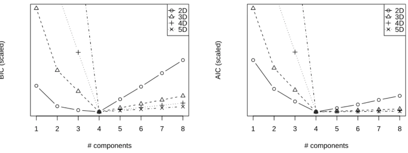
BIC for Tensor16 data
# components BIC (scaled) 2D 3D 4D 5D 1 2 3 4 5 6 7 8
AIC for Tensor16 data
# components AIC (scaled) 2D 3D 4D 5D
Figure 1: AIC and BIC for Tensors of increasing dimensions (2 to 5), rescaled so that the minimum is at the same level. All suggest correctly 4 components as the right model size.
Under the null hypothesis of no difference between the two models, LR is approximately asymptotically chi-square distributed, with a number of degrees of freedom, df , equal to the difference in the number of parameters in the two models. In the three dimensional case, for example, df = (R2− R1)(I + J + K − 2).
This suggests the following model selection strategy: Starting from R = 1, a) Estimate model bθR with
R component; b) Estimate model bθR+1 with R + 1 components; c) Repeat previous step as long as
2(L(bθR+1) − L(bθR)) > χ2(1 − α, (I + J + K − 2)). Notice that the number of degrees of freedom between
successive models is always the same as it corresponds to adding a single component, so we essentially compare the increase in log-likelihood obtained from each new component to a fixed threshold χ2(1−α, df ).
3
Experiments
Testing model selection is typically done at either side of a compromise: using artificial data on which the “right” model structure is known, a slightly favorable situation, or using real data, which provides a more realistic setting, but where the correct model structure is unknown. As an illustration, we use the former: we generate several datasets of various dimensions and size, each using 4 factors/components. Factors are overlapping “waves” over either 16 or 24 modalities. We obtain seven datasets: from 16 × 16 to 16 × 16 × 16 × 16 × 16 (1 million cells) and from 24 × 24 to 24 × 24 × 24 × 24 tensors.
On each of these 7 arrays, we computed the PTF with R = 2 to R = 8 components and computed the BIC/AIC criteria and likelihood ratio at each stage. These were estimated using a deterministic annealing variant of EM and multiple random restarts in order to diminish the influence of local minima of the loss function. Figure 1 shows how BIC/AIC behave as the number of components is increased for the 2-to-5-dimensional tensors with 16 modalities. In all cases, the minimum of the information criteria suggest the correct model size of 4 factors. It is apparent that, as expected, BIC penalizes additional components more than AIC. The rate of decrease or increase of the information criteria also varies depending on the data size and dimensionality.
In order to obtain a threshold χ2(1−α, df ) on the chi-squared statistic, we choose the traditional α = 0.05,
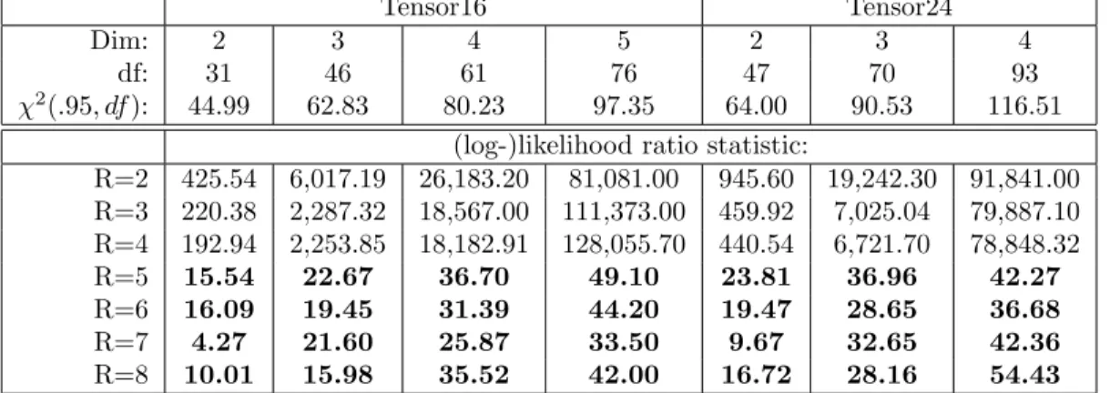
although other reasonable values of α yield essentially the same result. Depending on the size of the data, and on the difference in degrees of freedom (second row of Table 3), this gives different thresholds, as indicated in the third row of the table. In all cases we see that the observed log-likelihood ratio statistic (lower part of the table) is above the threshold until we reach R = 4 factors, and below when we add components beyond that. This again suggests (correctly) that the proper number of factors for these example tensors is 4.
Tensor16 Tensor24
Dim: 2 3 4 5 2 3 4
df: 31 46 61 76 47 70 93
χ2
(.95, df ): 44.99 62.83 80.23 97.35 64.00 90.53 116.51 (log-)likelihood ratio statistic:
R=2 425.54 6,017.19 26,183.20 81,081.00 945.60 19,242.30 91,841.00 R=3 220.38 2,287.32 18,567.00 111,373.00 459.92 7,025.04 79,887.10 R=4 192.94 2,253.85 18,182.91 128,055.70 440.54 6,721.70 78,848.32 R=5 15.54 22.67 36.70 49.10 23.81 36.96 42.27 R=6 16.09 19.45 31.39 44.20 19.47 28.65 36.68 R=7 4.27 21.60 25.87 33.50 9.67 32.65 42.36 R=8 10.01 15.98 35.52 42.00 16.72 28.16 54.43
Table 1: Log-likelihood ratio statistic and χ2 test. Dim: dataset dimension; df : degrees of freedom;
χ2(.95, df ): test threshold. Values below threshold (bold) indicate that the new component is unnecessary.
Note again that these results were obtained on artificially generated data where the proper model structure is known. The outcome is usually less clear-cut on a real dataset. However these results suggest that these criteria, inspired by the probabilistic model, may at least give a useful indication of a suitable model structure.
4
Conclusion
The probabilistic view of Positive Tensor Factorization is a straightforward extension of the 2D relationship between NMF and PLSA. Nevertheless, it has some interesting implications in terms of normalizing or estimating the factored representation. Using information criteria and likelihood ratio tests, we saw that it is possible to accurately select the number of factors in a situation where the model is complete, ie, there is a model instance that does generate the data. We hope that this relationship can be exploited to further the understanding and help the use of positive tensor factorization.
Acknowledgements: We acknowledge the help of Anicet Choupo with running some of the experiments.
References
[1] H. Akaike. A new look at the statistical model identification. IEEE Tr. Automatic Control, 19(6):716-723, 1974.
[2] W. Buntine. Variational extensions to EM and multinomial PCA. In ECML’02, pages 23-34, 2002. [3] E. Gaussier and C. Goutte. Relation between PLSA and NMF and implications. In SIGIR: 601–602, 2005. [4] C. Goutte, E. Gaussier, K. Yamada. Aligning words using matrix factorisation. In ACL: 502–509, 2004. [5] T. Kolda. Multilinear operators for higher-order decompositions. T.R. SAND2006-2081, 2006.
[6] D.D. Lee and H.S. Seung. Learning the parts of objects by non-negative matrix factorization. Nature, 401:788-791, 1999.
[7] D.D. Lee and H.S. Seung. Algorithms for non-negative matrix factorization. In NIPS’13. MIT Press, 2001. [8] M. Mørup, L.K. Hansen, J. Parnas, and S.M. Arnfred. Decomposing the time-frequency representation of EEG
using non-negative matrix and multi-way factorization. T.R., Informatics and Mathematical Modeling, 2006. [9] P. Paatero and U. Tapper. Positive matrix factorization: A non-negative factor model with optimal utilization
of error estimates of data values. Environmetrics 5:111-126, 1994.
[10] P. Paatero. A weighted non-negative least squares algorithm for three-way ’PARAFAC’ factor analysis. Chemometrics and Intel. Lab. Sys., 38:223-242, 1997.
[11] G. Schwartz. Estimating the dimension of a model. The Annals of Statistics, 6(2):461-464, 1978.
[12] M. Welling and M. Weber. Positive tensor factorization. Pattern Recognition Letters, 22(12):1255-1261, 2001.