Publisher’s version / Version de l'éditeur:
ASME 2016 35th International Conference on Ocean, Offshore and Arctic
Engineering, Volume 3, Structures, Safety and Reliability, p. V003T02A047,
2016-06
READ THESE TERMS AND CONDITIONS CAREFULLY BEFORE USING THIS WEBSITE. https://nrc-publications.canada.ca/eng/copyright
Vous avez des questions? Nous pouvons vous aider. Pour communiquer directement avec un auteur, consultez la première page de la revue dans laquelle son article a été publié afin de trouver ses coordonnées. Si vous n’arrivez pas à les repérer, communiquez avec nous à [email protected].
Questions? Contact the NRC Publications Archive team at
[email protected]. If you wish to email the authors directly, please see the first page of the publication for their contact information.
NRC Publications Archive
Archives des publications du CNRC
This publication could be one of several versions: author’s original, accepted manuscript or the publisher’s version. / La version de cette publication peut être l’une des suivantes : la version prépublication de l’auteur, la version acceptée du manuscrit ou la version de l’éditeur.
For the publisher’s version, please access the DOI link below./ Pour consulter la version de l’éditeur, utilisez le lien DOI ci-dessous.
https://doi.org/10.1115/OMAE2016-54329
Access and use of this website and the material on it are subject to the Terms and Conditions set forth at
Deformation of the wave field interacting with offshore platforms:
comparison between the corresponding results from a numerical
model and a wave tank
Zaman, M. Hasanat; Akinturk, Ayhan
https://publications-cnrc.canada.ca/fra/droits
L’accès à ce site Web et l’utilisation de son contenu sont assujettis aux conditions présentées dans le site LISEZ CES CONDITIONS ATTENTIVEMENT AVANT D’UTILISER CE SITE WEB.
NRC Publications Record / Notice d'Archives des publications de CNRC:
https://nrc-publications.canada.ca/eng/view/object/?id=b41fd364-db02-490c-af78-ed0a35343e8e https://publications-cnrc.canada.ca/fra/voir/objet/?id=b41fd364-db02-490c-af78-ed0a35343e8eProceedings of the ASME 2016 35th International Conference on Ocean, Offshore and Arctic Engineering OMAE2016 June 19 - June 24, 2016, Busan, South Korea
OMAE2016-54329
DEFORMATION OF THE WAVE FIELD INTERACTING WITH OFFSHORE
PLATFORMS
– COMPARISON BETWEEN THE CORRESPONDING RESULTS
FROM A NUMERICAL MODEL AND A WAVE TANK
M Hasanat Zaman Ayhan Akinturk
National Research Council Canada National Research Council Canada Ocean, Coastal and River Engineering Ocean, Coastal and River Engineering
Arctic Ave., PO Box 12093, Station A Arctic Ave., PO Box 12093, Station A St. John's, NL, A1B 3T5, Canada St. John's, NL, A1B 3T5, Canada
ABSTRACT
In the present research, a 3D dispersive numerical model has been developed and utilized to study the modification of the wave field in the presence of offshore structure. The Alternating Direction Implicit (ADI) algorithm has been employed for the solution of the governing equations. Relevant experiments are carried out in the Offshore Engineering Basin (OEB) of National Research Council (NRC) Canada. OEB is a 3D heavy duty 75m X 32m X 2.8m test facility equipped with modern data acquisition and tracking devices to record experimental data. Total 10 wave probes are deployed to measure the data at different locations in the Basin. Later the numerical results are compared with the experimental results. The comparisons of the numerical results show great agreement with the experimental results.
KEYWORD
Wave-structure interaction, 3D numerical model, experiments, data comparisons.
INTRODUCTION
In recent years the production and consumption of energy increases worldwide to keep up with the industrial development and is getting harder every day to ensure the optimum supply of energies in maintaining industrial activities smooth. Oil and gas
companies are continuously searching for new reservoirs in land and in the offshore region to meet the ever growing energy needs. Oceans are already identified as one of the comprehensive sources of hydrocarbon and renewable energy system. Renewable energy can be generated using ocean and tidal currents and waves using appropriate converters. Offshore wind turbine arrays are already in use to convert wind energy into electric energy. Hydrocarbon based offshore oil and gas companies are using FPSO to extract oil from relatively small reservoirs in the ocean but for larger reservoirs companies are widely relying on the gravity based structures (GBS) constructed in-situ or towed out to the location. Planning, design, construction, stability and operation of such structures depend highly on the local ocean environment. There are numerous scientific papers and publications are available in public domain that describe many aspects of the coexistence of the wave-current fields and GBSs. Just a few are mentioned here to represent some common scenarios. Thanyamanta et al (2011) using CFD code Flow 3D, describe the modification of the wave field and their consequent hydrodynamic loads on a GBS. Buchner et al (2004) describe the hydrodynamic loads on the moored vessels (LNG) due to the presence of a GBS. Bos et al (2002) present results of research about scour around large scale submerged offshore structures (Gravity Based Structures) subjected to the combined effect of loads related to waves and currents. They carried out model tests with a GBS protected by thick layers of various rock sizes, different hydraulic conditions and structure configurations. Roos et al (2010) describe the results of an experimental study of a gravity based structure in a
severe wave climate. Zaman and Baddour (2014) report the effects of the combined wave-current field on the offshore structures in a 3D flow field. In this work a 3D numerical model is developed and utilized to predict the wave deformation around the central shaft (see Fig.2) of the GBS assumed to be the crucial component of the offshore oil and gas platform. The basic physics of the numerical model uses the concept of the depth averaged velocity distribution along with an enhanced dispersion relation. The model is employed to study the propagation, reflection and diffraction of an incoming wave field in the presence of single-shaft and four-shaft GBSs in the deep and in the shallower water region. This study will provide us with more information that will help to better understanding the wave impact on ocean structures and thereby would help the industries to better planning, design and implementation of such ocean structures. The numerical results obtained from the model are compared with the relevant experimental results carried out in the OEB.
GOVERNING EQUATIONS
The following continuity equation and the equations of motion are utilized in the formulation of the model:
0 x y t P Q (1)
x y x xx yy t P P Q P P D f P gD D PQ D P P 2 2 2 2 2
B h Pxxt Qxyt Bah xxx xyy hhx Pxt Qyt hhy Qyt
6 1 6 1 3 1 3 1 2 3
hx xx yy hy xy
Bgh2 2 (2)
x y y xx yy t Q P Q Q Q D f Q gD D Q D PQ Q 2 2 2 2 2
B h Qyyt Pxyt Bah yyy xxy hhy Qyt Pxt hhx Pyt
6 1 6 1 3 1 3 1 2 3
hy yy xx hx xy
Bgh2 2 (3) r s r D Q Q Q Q d g gd tan ˆ 2 (4) 3 ) tan 3 . 5 57 . 0 ( 4 . 0 gd Qs (5) 3 135 . 0 gd Qr (6)
cosh( / ) 1
; j 1,2 ) (sinh 2 m Xj F j (7) 2 2 3 1 2 2 2 ) ( 1 1 h k B h Bk gh c (8)In the above equations, is the instantaneous water surface elevation, P the depth integrated velocity component or flux in the x-direction, Q the depth integrated velocity component or flux in the y-direction, h the local still water depth, D (=h+)
the local instantaneous water depth, g the gravitational acceleration, j the boundary damping function varies linearly
along the width of the sponge layers and null elsewhere, (Sato et al., 1992, Bayram and Larson, 2000, Zaman and Fraser, 2014) the eddy viscosity describes the momentum exchange due to turbulence, f the energy dissipation coefficient and the subscripts x, y and t denote the differentiation with respect to space and time. The parameter B is an important factor in the dispersion relation that depreciates the computational error in the wave celerity and group velocity. D is a coefficient (2.5 in
the surf zone and null elsewhere), tan the bottom slope, d the mean water depth and is the angular frequency.
Qˆ
is the flow amplitude, Qs the wave induced flow inside the surf zone and Qris the flow amplitude of the reform waves. The term j is the
boundary damping function and is null elsewhere apart from the boundary,
m gh, is a coefficient, F is the width of the sponge layer and Xj is the horizontal distance along the spongelayer in the x and y directions, respectively. In the numerical computation we have adopted = 1. In this computation sponge layer is introduced to eliminate or reduce any reflection from the beach. In the equations the wave number k is the wave number and c is the wave celerity. The wavenumber would be evaluated from the dispersion relation mentioned in Eq. (8) in which B is equal to 1/15 corresponds to the frequency dispersion obtained from Padé’s (2,2) expansion of the Stoke’s first-order theory.
NUMERICAL MODEL
The governing equations Eq.1 to Eq.3 are discretized following the mesh shown in Fig.1. For the solution of the governing equations a Finite difference numerical scheme is adopted that follows Alternating Directional Implicit algorithm or ADI method. The discretized equations are not shown here however, for details please refer to Zaman et al. (2000, 2001).
Fig. 1 Computational mesh y j )1 ( y j ) ( 2 1 y j y j )1 ( y j ) ( 2 1 x i )1 ( (i )x 2 1 ix (i )x (i )1x 2 1 P P P P P P Q Q Q Q Q Q x
y
DESCRIPTION OF THE EXPERIMENTAL SETUP
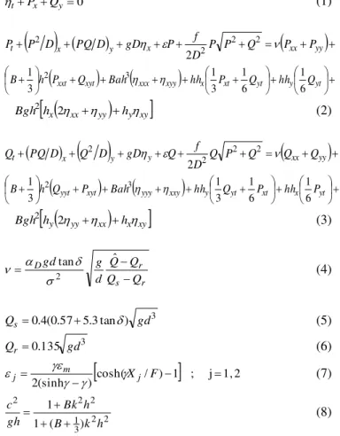
The Offshore Engineering Basin (OEB) of National Research Council is a world class heavy duty 3D wave testing facility. This basin is being used by the national and international clients to carry out different test projects. The experiments were carried out here in the OEB. The plan view of the basin is shown in Fig. 2. The Offshore Engineering Basin is 75 m long x 32 m wide. 56 independently controlled segmented wave generators installed on the west wall generated the waves. Each segmented wave generator is 2 m high and 0.5 m wide. Passive absorbers, made of expanded metal sheets with varying porosities and spacing, are installed on the east wall. A solid metal wall is used to cover the north side of the basin. The water depth for the experiments was 0.8m. During the experiment, total 10 wave probes were used but only 5 are shown (by ) in Fig. 2 where data comparisons are carried out. Table 1 shows the location of the wave probes in the basin. All the wave probes are capacitance type. Table 2 shows the locations of the shafts of the GBS (S1-S2-S3-S4) in the basin. Each shaft is of square cross-section with 0.8m sides. All the data was acquired using GDAC (GEDAP Data Acquisition and Control) client-server acquisition system, developed by National Research Council Canada.
Table 1 Location of the wave probes in the OEB Probe
number
Distance from the west wave paddle
(m)
Distance from the south wall
(m) 14 17.526 12.751 13 21.632 8.716 12 11.557 8.697 3 24.756 12.758 9 31.651 12.754
Table 2 Location of the shafts in the OEB
Shaft of GBS
Distance from the east wave
paddle (m)
Distance from the south wall
(m) Shaft 1 (S1) 24.697 8.672 Shaft 2 (S2) 24.715 16.803 Shaft 3 (S3) 20.619 12.762 Shaft 4 (S4) 28.766 12.742
BOUNDARY CONDITIONS AND ABSORBING BOUNDARY
Open boundary condition is adopted to make sure that the transmitted waves will go out of the domain and almost no reflection would take place from the beach to the computational domain. To replicate this condition we have introduced energy damping layer or sponge layer (see Eq. 7) over the transmitted region. This sponge layer is used to absorb all or most of the energy that penetrates into it and thus reduce the reflections from the beach. We did not introduce any sponge layer over the incident boundary in order to account for the effects of the reflected wave components from the structure(s) on the incident waves. A two-wavelength (2L) width of the sponge layer is required to absorb most of the wave energy incident to them. The wider the width of the sponge layer the better the accuracy of the final results. In case 4 and 5 sponge layers were introduced over side walls also shown in Figs. 9 and 10 to minimize reflections from the side walls.
Wave-makers South
Beach
Fig. 2: Layout of the experimental tank (not to scale) S1 S2 S4 S3 P-14 P-3 P-9 P-12 P-13
RESULTS AND DISCUSSIONS
In this work 3 different cases of regular waves over uniform water depth of 0.8m were considered for the comparisons of the experimental data with the numerical results for shallow water waves. Two different cases of deep water waves (hL0.5) were also included in the results and discussions. Table 3 shows the incident wave parameters of the wave conditions examined in this report. In the table T is the wave period, h is the still water depth, L is the wavelength, h/L is the relative water depth, H is the wave height and H/L is the steepness of the incident waves.
Table 3 Incident wave parameters
h (m) T (s) H (m) h/L H/L Shafts Case-1 0.8 1.436 0.15 0.26 5% None Case-2 0.8 1.436 0.15 0.26 5% S3 Case-3 0.8 1.436 0.15 0.26 5% S1,S2,S3 ,S4 Case-4 0.8 0.982 0.08 0.53 5% S3 Case-5 0.8 0.982 0.08 0.53 5% S1,S2,S3 ,S4
COMPARISONS OF NUMERICAL AND EXPERIMENTAL RESULTS
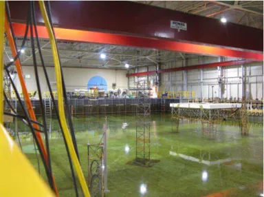
Fig. 3 shows the surface elevations computed by the numerical model and Fig.4 shows the comparisons of the numerical results with the experimental results of the surface elevations at probe locations P-14, P-13, P12, P-3 and P-9 for Case-1 when the bottom is essentially flat and no GBS is in presence. In Fig. 3 obtained results are normalized by the incident wave height. But normalization is not adopted for Fig. 4. It may be observed from the comparisons that numerical results show good agreement with the experimental results on the flat bottom.
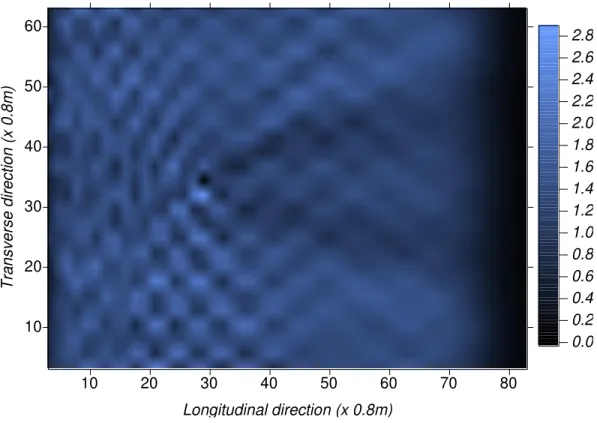
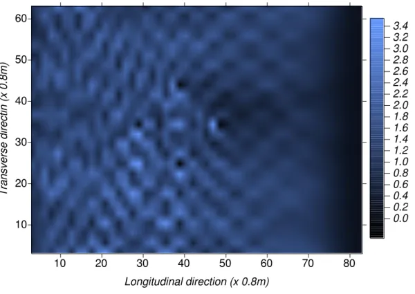
For Case-2, Fig. 5 shows normalized wave height in the whole domain and Fig. 6 compares numerical results with the experiments when shaft 3 (S3) is in presence on the flat bottom of the basin. In the figure comparisons are shown at the locations of Probes 14-13-12-3-9. Again for Case-3, Fig. 7 shows normalized numerical wave height in the whole domain and Fig. 8 shows similar comparisons at Probes 14-3-9-13-14 in the presence of shafts of the GBS S1-S2-S3-S4 on the flat bottom. On the other hand for deep water waves, shown by Case-4 and Case-5, Figs. 8 and 9 respectively show normalized wave heights due to shaft S3 and shafts S1-S2-S3-S4. In the presence of the shaft in the wave field, the flow condition becomes very complicated due to the inevitable reflected and diffracted waves. It is also observed that when all four shafts are in presence, some energy of the incoming wave fields get trapped inside the columns (see Figs. 7 and 10) that creates very unstable flow pattern over this area. From the above results it may be observed that numerical results agree very well with the experimental results in the presence or in the absence of single or multiple shafts in the wave field. More data analysis is being carried out for future comprehensive publications.
Sketch 1: Schematic view of the air gap experiments Photo 2: Testing of a single shaft GBS with high waves is in progress
Fig. 4 Comparisons between the numerical and measured surface elevations at five different locations in the OEB (Case 1: h=0.8m, H=0.15m, T=1.436s, h/L=26.7% and H/L=5%, no shaft is in presence
10 20 30 40 50 60 70 80 Longitudinal direction (x 0.8m) 10 20 30 40 50 60 T ra n s v e rs e d ir e c tio n ( x 0 .8 m ) -0.5 -0.4 -0.3 -0.2 -0.1 -0.0 0.1 0.2 0.3 0.4 0.5
Fig. 3 Bird’s view of the surface elevations obtained from the numerical model, normalized by the incident wave height (Case 1: h=0.8m, H=0.15m, T=1.436s, h/L=26.7% and H/L=5%, no shaft is in presence
Fig. 5 Bird’s view of the surface elevations obtained from the numerical model, normalized by the incident wave height (Case 2: h=0.8m, H=0.15m, T=1.436s, h/L=26.7% and H/L=5%, single shaft S3 is in presence
Fig. 6 Comparisons between the numerical and measured surface elevations at five different locations in the OEB (Case 2: h=0.8m, H=0.15m, T=1.436s, h/L=26.7% and H/L=5%, single shaft S3 is in presence
10 20 30 40 50 60 70 80 Longitudinal direction (x 0.8m) 10 20 30 40 50 60 T ra n s v e rs e d ir e c ti o n ( x 0 .8 m ) 0.0 0.2 0.4 0.6 0.8 1.0 1.2 1.4 1.6 1.8 2.0 2.2 2.4 2.6 2.8
Fig. 7 Bird’s view of the surface elevations obtained from the numerical model, normalized by the incident wave height (Case 3: h=0.8m, H=0.15m, T=1.436s, h/L=26.7% and H/L=5%, shafts S1-S2-S3-S4 is in presence
Fig. 8 Comparisons between the numerical and measured surface elevations at five different locations in the OEB (Case 3: h=0.8m, H=0.15m, T=1.436s, h/L=26.7% and H/L=5%, shafts S1-S2-S3-S4 is in presence
10 20 30 40 50 60 70 80 Longitudinal direction (x 0.8m) 10 20 30 40 50 60 T ra n s v e rs e d ir e c ti n ( x 0 .8 m ) 0.0 0.2 0.4 0.6 0.8 1.0 1.2 1.4 1.6 1.8 2.0 2.2 2.4 2.6 2.8 3.0 3.2 3.4
10.0 20.0 30.0 40.0 50.0 60.0 70.0 80.0 90.0 X - direction (x 0.8m) 10.0 20.0 30.0 40.0 Y d ir e c ti o n ( x 0 .8 m ) 0.00 0.25 0.50 0.75 1.00 1.25 1.50 1.75 2.00 2.25 2.50 10.0 20.0 30.0 40.0 50.0 60.0 70.0 80.0 90.0 X - direction (x 0.8m) 10.0 20.0 30.0 40.0 Y d ir e c ti o n ( x 0 .8 m ) 0.00 0.25 0.50 0.75 1.00 1.25 1.50 1.75
Fig. 9 Bird’s view of the surface elevations obtained from the numerical model, normalized by the incident wave height (Case 4: h=0.8m, H=0.15m, T=0.982s, h/L=0.53% and H/L=5%, single shaft S3 is in presence
Fig. 10 Bird’s view of the surface elevations obtained from the numerical model, normalized by the incident wave height (Case 5: h=0.8m, H=0.15m, T=0.982s, h/L=0.53% and H/L=5%, shafts S1-S2-S3-S4 is in presence
CONCLUSIONS
The reported model is capable to study the wave propagation, reflection and diffraction due to the presence of any ocean structures in a 3D flow field. This model is also efficient to incorporate wave breaking phenomenon in the numerical simulation. In this work only regular waves are reported but the model can be used to simulate irregular waves as well. The comparisons of several results between the model and the experiments show good agreement during the presence or absence of the structures, resemble to offshore platform’s shaft. From the obtained results it is perceived that this model can efficiently identify the locations of relatively low wave height zones in the hind side of the structure. This low wave height zones could be used to safe launch of the life boats when necessary during any emergency evacuation process. This is very important to ensure safety to the human lives. This paper shows part of the results of the whole numerical and experimental works. The rest of the results would be published somewhere else.
REFERENCES
Bayram, A. and M. Larson (2000): Wave transformation in the nearshore zone: comparison between a Boussinesq model and field data, Coastal Engineering, Elsevier, 39, pp.149-171. Bos, K. J, Verheij1, H. J., Kant, G. and Kruisbrink, A.C.H. (2002): Scour protection around gravity based structures using small size rock, Ist Int. conf. on Scour of Foundation, ICSF-1, Texas A & M University, College Station, Texas, USA, pp 17-20.
Buchner, B., Loots, G.E and Forristal, G.Z (2004): Hydrodynamics aspects of Gravity Based Structures as LNG import terminal in shallow water, OTC Conference, Houston, OTC2004-16716.
Roos, J., Swan, C and Haver, S. (2010): Wave impacts on the column of a gravity based structure, OMAE2010-20648, pp 365-373.
Sato, S., M. Kabiling and H. Suzuki (1992): Prediction of near bottom velocity history by a non-linear dispersive wave model, Coastal Engineering in Japan 35(1), pp.68-82.
Thanyamanta, W., Herrington, P. and Molyneus, D. (2011): Wave patterns, wave induced forces and moments for a gravity based structure predicted using CFD, OMAE2011-49593. Zaman, M. H. and Baddour, E. (2014): Loading due to interaction of waves with collinear and oblique currents, Ocean Engineering, 81(2014), pp 1-11.
Zaman, M. H, Hirayama, K. and Hiraishi, T. (2001): An extended Boussinesq model and its application to long period waves. Proc. 11th Int. Offshore and Polar Eng. Conf., ISOPE-2001, Stavanger, Norway, Vol. III, pp.607-614.
Zaman, M. H, Hirayama, K. and Hiraishi, T. (2000): A Boussinesq Model to Study Long period waves in a harbor. Report of the Port and Harbor Research Institute, Japan. Vol.39, No.4, pp.25-50.
Zaman, M. H., Winsor, F. (2014): A 3D wave model to simulate the interaction of wave field in the presence of multi-structures. OCEANS'14 MTS/IEEE, 14-19 September, 2014, St. John's, NL, Canada.