Autonomous orbital rendezvous using angles-only navigation

AUTONOMOUS ORBITAL RENDEZVOUS USING ANGLES-ONLY NAVIGATION by

Raja Jon Vurputoor Chari

B.S. Astronautical Engineering United States Air Force Academy, 1999

B.S. Engineering Sciences United States Air Force Academy, 1999

SUBMITTED TO THE DEPARTMENT OF AERONAUTICS AND ASTRONAUTICS IN PARTIAL FULFILLMENT OF THE REQUIREMENTS FOR THE DEGREE OF

MASTER OF SCIENCE IN AERONAUTICS AND ASTRONAUTICS at the

MASSACHUSETTS INSTITUTE OF TECHNOLOGY June 2001

© 2001 Raja Jon Vurputoor Chari. All rights reserved.

The author hereby grants to MIT permission to reproduce and to distribute publicly paper and electronic copies of this thesis document in whole or in part.

Signature of Author_

/1'

{/

Approved by

7o/

Department of Aeronautics and Astronautics

May 11, 2001

David K. Geller

Charles Stark Draper Laboratory, Inc. Technical Supervisor

Certified by

John J. Deyst, Jr. Professor of Aeronautics and Astronautics

Thesis Advisor

/ I n A

Accepted by

AUTONOMOUS ORBITAL RENDEZVOUS USING ANGLES-ONLY NAVIGATION by

Raja Jon Vurputoor Chari

Submitted to the Department of Aeronautics and Astronautics on May 11, 2001 in Partial Fulfillment of the Requirements for the Degree of Master of Science in Aeronautics and Astronautics

Abstract

This study assesses navigation performance for rendezvous and close approach applications where on-board navigation must be accomplished through the use of angles-only measurements by developing various relative motion orbital trajectories. Chaser vehicle maneuvers designed to enhance the estimator's observability of the downrange distance to the target are considered. The target vehicle is assumed to be non-maneuvering and in a near-circular

orbit. The modeled system includes representative scenarios from the Orbital Express mission. Although a wide array of angle measurement sensors are available, their use in orbital rendezvous is generally limited by the fact that they are unable to provide direct target ranging information which leads to significant downrange error accumulation in the navigation filter. These navigation problems inherent to angles-only measurements in a natural motion environment are first qualitatively studied both analytically and through linear covariance

modeling. It is shown that different target-chaser geometries lead to different navigation

uncertainties in target downrange distance. The conclusions drawn from considering natural motion geometries are used to study candidate maneuver-assisted trajectories. The results from this study are used to select and combine the most promising maneuver-assisted trajectories for

more in-depth consideration as potential scenarios for the Orbital Express mission. These

selected trajectories are then analyzed in depth to determine the interdependency of range observability using angles-only navigation with angular sensor quality, inertial measurement

accuracy, attitude determination accuracy, and trajectory design. Using the Orbital Express

mission as a baseline, maneuver-assisted trajectories for angles-only navigation are tested with realistic error models to validate the rules of thumb created for improved angles-only navigation even in the presence of biases, misalignments, and degraded sensors. The results show that using well-chosen trajectories leads to navigation error uncertainties acceptable for rendezvous applications when only angular measurements are available.

Technical Supervisor: Dr. David K. Geller

Title: Senior Member of the Technical Staff, Charles Stark Draper Laboratory, Inc. Thesis Advisor: John J. Deyst, Jr.

ACKNOWLEDGMENT

(May 11, 2001)

"If I have seen further it is by standing upon the shoulders of giants." - Isaac Newton

This thesis came about only through the time and help of a number of people and

organizations. Thanks to the Charles Stark Draper Laboratory, the Air Force Institute of

Technology, and the Massachusetts Institute of Technology for making this program possible. I would like to thank all the staff at Draper Laboratory that I worked with over the last two

years. First and foremost, thanks to Dr. David Geller, I couldn't have asked for a better

supervisor. I'm not sure how I wound up being so lucky. He was a wonderful mentor and friend, and somehow managed to have the patience to put up with my near daily questions. Thanks for your tireless support, and the countless number of extra hours you spent at the lab helping to guide me along. Just to re-emphasize this point, I couldn't have had a better supervisor. I'm also grateful to Tim Brand for his suggestions and back-of-the-envelope ideas that helped to make this a better thesis. Thanks to Chris D'Souza, Lee Norris, and Peter Kachmar for getting me involved in the Mars Sample Return work, and for your encouraging help and wisdom throughout my time here. Thanks to George Schmidt and the education office for providing me with the opportunity to work at Draper, and thanks to Chris Stoll, Ron Proulx, and Paul Cefola who helped me get my feet wet upon first arriving at the lab.

My deepest thanks also go to the staff and incredible professors at MIT for giving me the knowledge and skills to accomplish this study. I especially thank Dr. John Deyst for his role as my advisor helping to keep me on course and providing critical insights throughout my research.

Thanks also to those who shared in my experiences as a Draper fellow. To my

ex-officemate George Granholm, thanks for teaching me the ropes and providing late night study break entertainment. I also thank my new officemate, Ted Dyckman for putting up with my conversations and being a bottomless source of intriguing information. Thanks to my next-door cubicle buddies Paul Goulart, Jeremy Rea, and Andrew Grubler although I won't miss living in fear of nocturnal office pranks. Also, thanks to Rich Shertzer and Steve Clark for being my lunch-time comrades and fellow Wednesday uniform wearers.

guys. Have fun keeping up the reputation of 16 Clinton St., frequent the Phoenix Landing often in my honor, and go Red Sox (this is definitely their year).

Besides the people here in Boston, I would like to thank my family for always welcoming me home for much needed breaks and for their unconditional love and support. They have made

me the person I am today. Happy 25h anniversary mom and dad, enjoy having the house to

yourselves and Krishna, good luck beginning the college experience. Thanks also to the friends, faculty, and staff from St.Patrick's elementary school, Columbus high school, and the Air Force Academy who helped to mold me and continue to take an interest in my work today.

To my fianc6e, Holly, thanks for being you and bringing out the best in me. Your love continues to inspire and motivate me. Thanks for sticking by me through thick and thin, and being a part of my daily life despite the physical distance between us. I look forward to spending the rest of my life with you.

Last, but surely not least, I thank God for blessing me with the people who surround me and endowing me with talents that allowed me to complete this work.

"Two roads diverged in a wood and I - I took the one less traveled by, and that has made all the difference." - Robert Frost

This thesis was prepared at The Charles Stark Draper Laboratory, Inc., under Internal Research and Development Project 13088, Rendezvous with Angles-Only Navigation.

Publication of this thesis does not constitute approval by Draper or the sponsoring agency of the findings or conclusions contained herein. It is published for the exchange and stimulation of ideas.

Table of Contents

S

1.1 PROBLEM BACKGROUND AND M OTIVATION ... 21

1.2 THESIS OVERVIEW ... 22

1.3 ASSUMPTIONS ... 23

2 AN A LY SIS TO O LS... 25

2.1 KALM AN FILTER FORMULATION ... 25

2.1.1 State and Covariance Propagation and Updating ... 26

2.1.2 Linearization... 29

D y n am ic s ... 3 0 M easurements...31

2.1.3 D erivation of M easurement Sensitivity M atrix ... 32

Partials with Respect to Target and Chaser Position... 35

Partials with Respect to Velocity and Angular M easurement Biases ... 37

Partials with Respect to Static M isalignment... 38

Partials with Respect to Inertial Attitude Error... 39

2.2 LINEAR COVARIANCE ANALYSIS ... 41

2.2.1 General Explanation and Setup ... 41

2.2.2 LINCO V M odels... 46

Un-modeled Accelerations ... 46

System Biases and First Order M arkov Processes ... 47

M aneuver M easurement Errors ... 47

2.2.3 Current Configuration ... 48

3 NATURAL MOTION RANGE OBSERVABILITY ... 51

3.1 BACKGROUND... 51

3.2 REFERENCE TRAJECTORY DEVELOPMENT... 53

3.2.1 Constraints... 53

3.2.2 Shifted Altitude M etric ... 55

3.2.3 Station-keeping ... 56

3.2.4 Closure... 60

3.3 LINEAR COVARIANCE RESULTS ... 65

3.3.1 Setup... 65

3.3.2 Station-keeping ... 66

Co-circular Orbits...67

3.4 ADDITIONAL ANALYSIS CONSIDERATIONS... 86

3.4.1 Error Ellipse Behavior... 86

Centered Station-keeping Football ... 88

Offset Station-keeping Football...90

C oellip tic ... 9 3 3.4.2 Measurement Availability ... :... 96

3.4.3 Noise Vs. Number of M easurements ... 98

3.4.4 Biases ... 100

3.5 GENERAL CONCLUSIONS... 104

3.5.1 Effects of M easurement Noise ... 106

3.5.2 A Priori Effects on Benefits of Geom etry ... 108

4 MANEUVER-ASSISTED TRAJECTORY ANALYSIS ... 113

4.1 COMPARISON TO PREVIOUS W ORK ... 113

4.2 REFERENCE TRAJECTORY DEVELOPMENT... 114

4.2.1 Station-keeping ... 115

4.2.2 Closure... 119

4.3 LINEAR COVARIANCE RESULTS ... 128

4.3.1 Station-keeping ... 129

4.3.2 Closure... 137

V-bar Approaches...137

R-bar Approaches...138

M odified Coelliptics ... 139

M odified Traveling Footballs ... 142

Effects of Process Noise ... 144

Results Summary...146

4.4 GENERAL CONCLUSIONS AND HYBRID TRAJECTORY DEVELOPMENT ... 147

5 M ISSIO N ANALY SIS...159

5.1 M ISSION OVERVIEW ... 159

5.2 INCORPORATION OF M ISSION SPECIFICATIONS... 161

5.3 DESIGN OF M ISSION TRAJECTORIES ... 164

5.3.1 Closure... 165

5.3.2 Station-keeping ... 170

5.4 RESULTS ... 172

5.4.1 End-to-End Testing ... 182

Dispersions Due to Velocity Uncertainty ... 185

Geo-Synchronous Test Case...187

6 CO N CLU SIO NS ... 189

6.1 SUMMARY OF RESULTS ... 189

6.1.2 M aneuver-Assisted Navigation ... 190

6.1.3 Orbital Express M ission Analysis ... 190

6.2 FuTURE W ORK... 190

6.2.1 D ispersion Analysis... 191

6.2.2 M onte Carlo Analysis... 191

6.2.3 Form ulation of problem in relative frame... 191

6.2.4 Observability Calculation ... 192

List of Figures

Figure 2-1: State and covariance propagation and updating ... 27

Figure 2-2: Filtering equations flow diagram ... 29

Figure 2-3: Angular measurements from chaser to target...32

Figure 2-4: Filter design using LINCOV analysis ... 45

Figure 3-1: Uncertainty with angular measurements and no relative geometry ... 52

Figure 3-2: Uncertainty with angular measurements and use of relative geometry...52

Figure 3-3: Target-centered LVLH coordinate frame... 54

Figure 3-4: Shifted altitude m ethod ... 55

Figure 3-5: Co-circular station-keeping 10km away with 10km of cross-track motion ... 57

Figure 3-6: Football station-keeping 100m away, 10m vertical motion with 10m of cross-track m o tio n ... 5 8 Figure 3-7: Football station-keeping centered on target, 1km vertical motion ... 59

Figure 3-8: Coelliptic with 10km Ah ... 61

Figure 3-9: V-bar hops with 1km Ah ... 62

Figure 3-10: Traveling football with 10m Ah and 100m of vertical motion with 10m of cross-track m otion ... 63

Figure 3-11: Inertial and relative RSS uncertainty for Co-circular station-keeping 1km away...67

Figure 3-12: Relative position uncertainty for Co-circular station-keeping 1km away ... 68

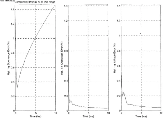
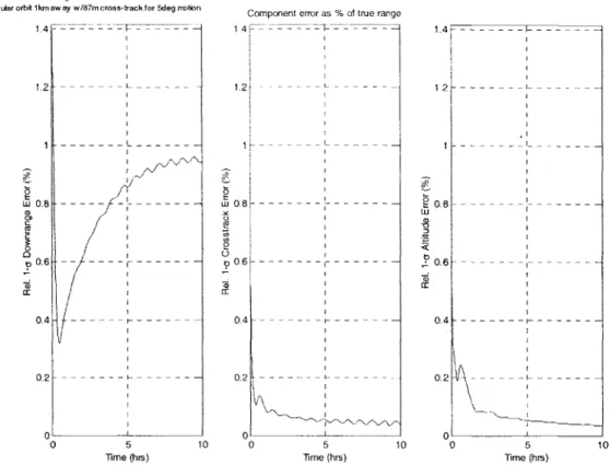
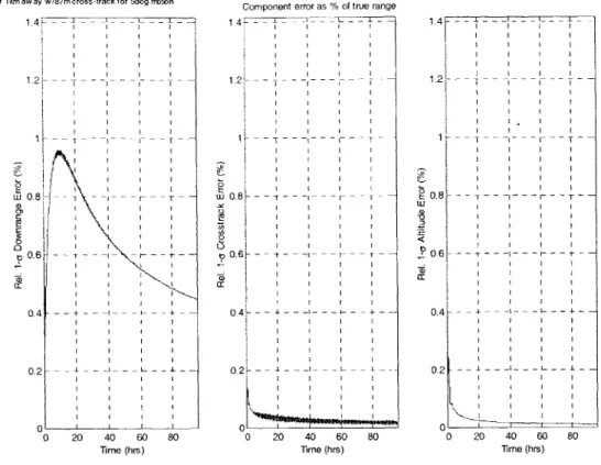
Figure 3-13: Relative position uncertainty for Co-circular station-keeping 1km away with 87m cross-track m otion ... 69 Figure 3-14: Relative position uncertainty over 4 days for Co-circular station-keeping 1km away

Figure 3-16: Relative position uncertainty for Co-circular station-keeping 1km away with 1km cro ss-track m otion ... 7 1 Figure 3-17: Station-keeping football relative motion schematic ... 72 Figure 3-18: Relative position uncertainty for Football station-keeping 100m away with 10m vertical m otion ... 73 Figure 3-19: Relative position uncertainty for Football station-keeping 300km away with 100km vertical motion and 100km cross-track motion... 74 Figure 3-20: Relative position uncertainty for Football station-keeping centered on target with 1km vertical m otion ... 75 Figure 3-21: Relative position uncertainty for Football station-keeping centered on target with

1km vertical motion and 1km cross-track motion...76 Figure 3-22: Coelliptic relative motion schematic...77

Figure 3-23:Actual relative position & velocity uncertainty values for Coelliptic with 100m Ah 78 Figure 3-24: Relative position uncertainty for Coelliptic with 100m Ah...79 Figure 3-25: Relative position uncertainty for Coelliptic with 1km Ah and 1km cross-track

m o tio n ... 80 Figure 3-26: Relative position uncertainty for Coelliptic with 1km Ah...80 Figure 3-27: V-bar hop relative motion schematic ... 81 Figure 3-28: Relative position uncertainty for V-bar hops with 1km Ah and 1km cross-track

m o tion ... 8 2 Figure 3-29: Relative position uncertainty for V-bar hops with 1km Ah...82

Figure 3-30: Traveling football relative motion schematic...83 Figure 3-31: Relative position uncertainty for Traveling football with 10m Ah and 100m vertical

m o tio n ... 84 Figure 3-32: Relative position uncertainty for Traveling football with 10m Ah and 100m vertical

motion with 10m cross-track motion ... 85 Figure 3-33: Relative position uncertainty for Traveling football with 10m Ah and 100m vertical

Figure 3-34: Two dimensional error ellipse dimensions...87

Figure 3-35: Incorrect expected error ellipse behavior for Centered station-keeping football...88

Figure 3-36: Expected error ellipse behavior for Centered station-keeping football...89

Figure 3-37: Correlation coefficient time history for Centered station-keeping football ... 90

Figure 3-38: Error ellipse behavior for Centered station-keeping football ... 90

Figure 3-39: Expected error ellipse behavior for Offset station-keeping football ... 91

Figure 3-40: Correlation coefficient time history for Offset station-keeping football...92

Figure 3-41: Error ellipse behavior for Offset station-keeping football... 92

Figure 3-42: Expected error ellipse behavior for Coelliptic... 93

Figure 3-43: Correlation coefficient time history for Coelliptic ... 94

Figure 3-44: Error ellipse behavior for Coelliptic... 94

Figure 3-45: Identical line-of-sight history for different coelliptic orbits... 95

Figure 3-46: Relative position uncertainty for Coelliptic with 100m Ah and increased a priori un certain ty ... 9 6 Figure 3-47: Measurements available only in sunlight - Actual relative position and velocity uncertainty values for Traveling football with 100m Ah and 1km vertical motion with 1km cross-track m otion ... 97

Figure 3-48: Measurements always available - Actual relative position and velocity uncertainty values for Traveling football with 100m Ah and 1km vertical motion with 1km cross-track m o tion ... 9 8 Figure 3-49: Actual relative position and velocity uncertainty values for V-bar hops with 1km A h ... 9 9 Figure 3-50: Increased noise and measurement frequency - Actual relative position and velocity uncertainty values for V-bar hops with 1km Ah...100 Figure 3-51: Actual relative position and velocity uncertainty values for Football station-keeping

Figure 3-53: Actual relative position and velocity uncertainty values for Football station-keeping 100m away with 10m vertical motion - Without biases...102

Figure 3-54: Filter bias value uncertainty for one bias -Football station-keeping 100m away with

10m vertical m otion ... 10 3

Figure 3-55: Filter bias value uncertainty for both biases - Football station-keeping 100m away

w ith 10m vertical m otion ... 104 Figure 3-56: Cone of equivalent relative motion geometries...105 Figure 3-57: Relative position and velocity uncertainty for Co-circular station-keeping 1km away

with 1km cross-track, 1/axis 3ca angular measurement noise...106 Figure 3-58: Relative position and velocity uncertainty for Co-circular station-keeping 1km away

with 1km cross-track motion, 50/axis 3ca angular measurement noise... 107 Figure 3-59: Relative position and velocity uncertainty for Co-circular station-keeping 1km away

with 1km cross-track motion, 0. 1/axis 3a angular measurement noise... 107

Figure 3-60: Relative position and velocity uncertainty for Co-circular station-keeping 1km away with 87m cross-track motion, normal a priori uncertainty ... 108 Figure 3-61: Relative position and velocity uncertainty for Co-circular station-keeping 1km away with 87m cross-track motion, increased a priori uncertainty ... 109 Figure 3-62: Relative position and velocity uncertainty over 4 days for Co-circular station-keeping 1km away with 87m cross-track motion, increased a priori uncertainty ... 110 Figure 3-63: Relative position and velocity uncertainty for Co-circular station-keeping 1km away

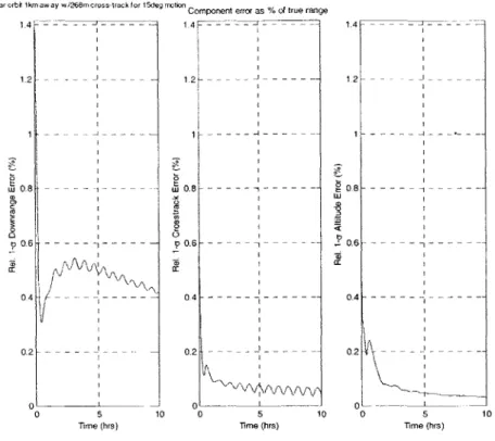
with 268m cross-track motion, normal a priori uncertainty ... 111 Figure 3-64: Relative position and velocity uncertainty for Co-circular station-keeping 1km away

with 268m cross-track motion, increased a priori uncertainty ... 11... 1

Figure 4-1: Football station-keeping 10m away with 1m vertical motion, 2.5 orbits of 1m cross-track m otion starting at 5 hours, AV =2mm/s ... 116 Figure 4-2: Co-circular station-keeping 100m away, 2.5 orbits of im cross-track motion starting

at 5 hours, A V =2m m /s...117 Figure 4-3: Football station-keeping centered on target with 100m vertical motion, 10m

Figure 4-4: V-bar approach from 360m at 1cm/sec with damped cross-track oscillations, A V = 1.59m /s ... 120 Figure 4-5: R-bar approach from 360m at lcm/sec with multiple observation maneuvers,

A V = 27 .lm /s ... 122

Figure 4-6:AV required for R-bar approaches with varying closing rates & initial separations.. 123 Figure 4-7: Coelliptic with 100m Ah and damped cross-track oscillations symmetric with respect

to flyby point from 2-8 hours, AV=8.85m/s...124 Figure 4-8: Traveling football with fixed 10m Ah and shrinking vertical oscillations with damped

cross-track oscillations, AV =1.85m /s...125 Figure 4-9: Traveling football with shrinking Ah and shrinking vertical oscillations,

A V = 0 .0 55m /s ... 12 6

Figure 4-10: Traveling football/spiral with shrinking Ah and shrinking vertical oscillations with multiple observation maneuvers, AV=1.55m/s ... 127 Figure 4-11: Relative position uncertainty for Football station-keeping centered on target with

100m vertical motion and 2.5 orbits of 10m cross-track motion starting at 5 hours,

A V = 0 .0 2m /s ... 130

Figure 4-12: Relative position uncertainty for Co-circular station-keeping 100m away with 2.5

orbits of 1m cross-track motion starting at 5 hours, AV=2mm/s ... 131

Figure 4-13: Relative position uncertainty for Co-circular station-keeping 100m away with 2.5 orbits of 10m cross-track motion starting at 5 hours, AV=.02m/s ... 131 Figure 4-14: Relative position uncertainty for Co-circular station-keeping 100m away with 2.5 orbits of 100m cross-track motion starting at 5 hours, AV=.2m/s ... 132 Figure 4-15: Relative position uncertainty for Football station-keeping 10m away with im vertical motion and 2.5 orbits of 10m cross-track motion starting at 5 hours, AV=0.02m/s 133 Figure 4-16: Relative position uncertainty for Football station-keeping 10m away with im vertical motion and 10m observation maneuvers starting at 5 hours, AV=0.32m/s...133

Figure 4-18: Relative position uncertainty with process noise for Co-circular station-keeping 100m away with 100m observation maneuvers every hour starting at 5 hours,

A V = 3 .2m /s ... 135

Figure 4-19: Maneuver-assisted station-keeping trajectory LINCOV results summary...137 Figure 4-20: Relative position uncertainty for V-bar approach from 360m at lcm/sec with 2 orbits

of 100m cross-track motion starting at 5 hours, AV=1.03m/s...138 Figure 4-21: Relative position uncertainty for R-bar approach from 360m at lcm/sec,

A V = 24 .4 m /s ... 139 Figure 4-22: Relative position uncertainties for Coelliptic with 100m Ah case with no cross-track

motion overlaid on case with damped cross-track oscillations symmetric with respect to

flyby point, A V =9.63m /s...140

Figure 4-23: Relative position uncertainty for Coelliptic with 100m Ah case with damped cross-track oscillations symmetric with respect to flyby point, AV=9.63m/s ... 141 Figure 4-24: Relative position uncertainty for Coelliptic with 1km Ah case with damped cross-track oscillations symmetric with respect to flyby point, AV=96.3m/s ... 141 Figure 4-25: Relative position uncertainty for Traveling football, unmodified, with 10m Ah and 100m vertical oscillations, AV =Om /s ... 142 Figure 4-26: Relative position uncertainty for Traveling football with shrinking Ah and shrinking vertical oscillations, AV =0.055m /s ... 143 Figure 4-27: Relative position uncertainty for Traveling football/spiral with shrinking Ah and shrinking vertical oscillations with multiple observation maneuvers, AV= 1.55m/s...144 Figure 4-28: Relative position uncertainty with process noise for Coelliptic with 100m Ah and

damped cross-track oscillations symmetric with respect to flyby point from 2-8 hours,

A V = 8.85m /s ... 145

Figure 4-29: Relative position uncertainty with process noise for Coelliptic with 100m Ah and multiple observation maneuvers, AV=50.72m/s ... 145

Figure 4-30: Maneuver-assisted closure trajectory LINCOV results summary ... 147

Figure 4-32: Hybrid trajectory 1 - R-bar final approach, AV=3m/s...150

Figure 4-33: Hybrid trajectory 1 - Relative position uncertainty for R-bar final approach, A V = 3 m /s ... 150

Figure 4-34: Hybrid trajectory 1 - V-bar final approach, AV=2.97m/s...151

Figure 4-35: Hybrid trajectory 1 - Relative position uncertainty for V-bar final approach to 17m, A V = 2 .97m /s ... 15 1 Figure 4-36: Hybrid trajectory 2- Spiral to final approach...152

Figure 4-37: Hybrid trajectory 2 - R-bar final approach, AV=1. 12m/s ... 153

Figure 4-38: Hybrid trajectory 2 - Relative position uncertainty for R-bar final approach to 8m, A V = 1.12 m /s ... 15 3 Figure 4-39: Hybrid trajectory 2 - V-bar final approach, AV=1.01m/s...154

Figure 4-40: Hybrid trajectory 2 - Relative position uncertainty for V-bar final approach to 32m, A V = 1.O lm /s ... 154

Figure 441: Hybrid trajectory 3- Centered football station-keeping to final approach...155

Figure 4-42: Hybrid trajectory 3 - R-bar final approach, AV=0.81m/s ... 156

Figure 4-43: Hybrid trajectory 3 - Relative position uncertainty for R-bar final approach, A V = 0 .8 1m /s ... 156

Figure 4-44: Hybrid trajectory 3 - V-bar final approach, AV=0.85m/s...157

Figure 4-45: Hybrid trajectory 3 - Relative position uncertainty for V-bar final approach to 8m, A V = 0 .85m /s ... 157

Figure 5-1: Orbital Express system elements...160

Figure 5-2: Orbital Express mission endpoints ... 161

Figure 5-3: Orbital Express trajectory option 1 schematic...166

Figure 5-8: Orbital Express trajectory testing results legend ... 174 Figure 5-9: Results for closure trajectories with quiet chaser vehicle using nominal error cases an d stress cases...17 8 Figure 5-10: Results for closure trajectories with noisy chaser vehicle using nominal error cases an d stress cases...17 9 Figure 5-11: Results for station-keeping trajectories with quiet chaser vehicle using nominal error cases and stress cases ... 180 Figure 5-12: Results for station-keeping trajectories with noisy chaser vehicle using nominal error

cases and stress cases ... 18 1 Figure 5-13: Orbital Express end-to-end trajectory schematic ... 183 Figure 5-14: End-to-end trajectory results for quiet chaser with all errors at nominal values and

varying measurement availability conditions...184 Figure 5-15: Relative position dispersions resulting from velocity uncertainty at maneuver

execution times for Orbital Express end-to-end trajectory ... 186 Figure 5-16: Geo-synchronous end-to-end trajectory results for quiet chaser with all errors at

List of Tables

Table 3-1: Natural motion station-keeping reference trajectories... 60

Table 3-2: Natural motion closure reference trajectories...64

Table 4-1: Maneuver-assisted station-keeping reference trajectories ... 119

Table 4-2: M aneuver-assisted closure reference trajectories ... 128

Table 4-3: Maneuver-assisted station-keeping trajectory LINCOV results summary ... 136

Table 4-4: Maneuver-assisted closure trajectory LINCOV results summary ... 146

Table 5-1: Summary of results for Orbital Express trajectories with quiet chaser vehicle...175

Introduction

1

INTRODUCTION

The purpose of this study is to make a qualitative and quantitative assessment of angles-only navigation performance for orbital rendezvous and close approach applications through the development and description of relative motion trajectories. This opening chapter addresses the background of the problem and the motivation for an angles-only approach. The following sections will present the major assumptions of the study and an overview of the remaining chapters.

1.1

PROBLEM BACKGROUND AND MOTIVATION

Although orbital rendezvous has been a well-studied problem since the Gemini era, it has

generally taken place with the benefit of a man-in-the-loop. A new generation of planned

missions such as the NASA Mars Sample Return Mission, ASTRO Orbital Express Project, and the Air Force's XSS- 11 are driving a demand for the ability to autonomously capture, inspect, or dock with on-orbit objects. Effective space rendezvous requires a navigation system to measure the relative position between the chaser and target vehicle. Measurement techniques used in the past include relative GPS (which requires a high degree of cooperation from the target spacecraft) or radar and lidar systems that can place significant power and weight requirements on the chaser. Additionally, the use of active sensing techniques is a stealthy approach in the case of a non-cooperative target.

In light of these drawbacks, angles-only relative navigation is an attractive alternative if adequate accuracy in all components of relative position can be achieved. Many simple sensors are capable of providing line-of-sight direction, such as optical or infrared cameras and trackers. Another attractive alternative is a radio direction finder, which only requires a simple radio frequency (RF) tone generator on the target. This technique, which has the potential to work at very long ranges as well as short distances, uses multiple antennas on the chaser to measure the

This thesis first seeks to study relative motion orbital trajectories that make the use of angles-only navigation feasible. In addition to trajectory design, though, there are a number of other factors that potentially affect the ability of a navigation system to accurately determine range along the line-of-sight including inertial measurement unit (IMU) accuracy, attitude determination accuracy, and the accuracy of the angular measurements themselves. Thus, as a secondary objective, the degrading effects of these error sources is examined using several selected trajectory designs and realistic error models based on the Orbital Express mission.

1.2

THESIS OVERVIEW

The ability to determine the distance along the line-of-sight is enhanced by a combination of two techniques. First, the relative motion trajectory between the chaser and target is designed to create changes in the line-of-sight, thereby enhancing the observability of all relative position components. Second, the chaser executes maneuvers which are designed to further enhance the observability of the position component along the line-of-sight.

Chapter 2 presents the linear covariance analysis tool used for this study and briefly covers

the basic navigation filtering equations. Chapter 3 qualitatively examines the navigation

problems inherent to angles-only measurements in natural motion orbital trajectories. A wide range of natural motion trajectories are considered across different operating ranges from meters

to hundreds of kilometers. The well-known problem of unbounded downrange uncertainty

growth in the navigation filter due to a lack of range observability when using only angular measurements is demonstrated. It is shown that changes in target-chaser relative geometry can decrease the navigation uncertainty of the target's downrange distance. A study of the evolution of the navigation uncertainties as functions of time shows their dependence on the line-of-sight motion associated with natural orbital mechanics, and motivates the use of maneuvers to sever this dependence. Additional factors such as measurement availability, measurement noise levels, a priori uncertainty values based on delivery conditions, and system biases are examined with regard to their interdependence and influence on the angles-only navigation problem.

Chapter 4 makes use of the conclusions drawn from considering natural motion trajectories to develop candidate maneuver-assisted trajectories. The maneuvers that create these trajectories are shown, and the trajectories themselves are briefly compared with results from dual-control literature. Based on performance analysis and a brief consideration of the effects of un-modeled accelerations, the most promising trajectories are selected for more in-depth consideration. Also,

Introduction

several hybrid trajectories are designed that combine the best characteristics of various approaches and create the basis for eventual mission testing.

Chapter 5 develops and tests several maneuver-assisted trajectories designed for the Orbital

Express mission environment. The analysis takes the chaser from its anticipated initial conditions

through final approach using realistic specifications for sensor models. These selected

trajectories are then explored to better understand and quantify the sensitivity of the navigation filter solution to different maneuver-assisted trajectories and un-modeled accelerations, as well as to IMU, attitude determination, and angular measurement errors. The results show that using well-chosen maneuver-assisted trajectories leads to navigation error uncertainties acceptable for rendezvous applications even when only angular measurements are available.

Chapter 6 presents conclusions drawn from the overall study and discusses potential topics for future work.

1.3

ASSUMPTIONS

For this study, it is assumed that the target and chaser vehicles are in nearly circular orbits since the vast majority of current potential rendezvous missions involve circular or near-circular orbits. Specifically, the author's work on the Mars Sample Return Mission and ASTRO Orbital Express Mission involved maximum eccentricity values of 0.04. Similarly, the current analysis considers only Low-Earth orbits (LEO) although the conclusions should easily extend to higher altitude orbits just as easily as they would extend to modestly elliptical orbits. The planetary constants for earth come from [16] although once again the extension of the results to other planetary central bodies would have no adverse effects.

The other major assumption is that higher order gravity terms, including J2, are not considered in the current analysis. The differential effects of such terms on target and chaser vehicles in close proximity are generally negligible. When this is not the case, the higher order terms should improve the results since they will introduce additional motion into the relative motion trajectory. There are a number of additional assumptions throughout this work that will be mentioned as they are made and used.

Analysis Tools

2

ANALYSIS TOOLS

This chapter covers the development of the tools that will be employed for analysis of the angles-only navigation problem. First, a general review of the equations governing Kalman filtering is presented, and then the topic is expanded to briefly explain the principles behind linear covariance (LINCOV) analysis. Finally, some of the more specific implementation issues as they pertain to this problem are addressed.

2.1

KALMAN FILTER FORMULATION

The concept of Kalman filtering was first put forward by R.E. Kalman in 1960. The idea is to create a recursive algorithm that is capable of processing measurements that are corrupted by errors. Ideally, one would like to know the exact values of state variables over time. However, in practice this is usually not possible, so the next best option is to estimate these values in a least squares optimal fashion. The Kalman filter equations provide a methodology to do exactly that in the case of linear systems.

Kalman filtering caught on quickly as it had immediate applications to guidance and navigation problems, specifically within the Apollo space program. Since then, the original algorithm, along with many variations, has been applied to numerous situations where it is desirable to know the state of a dynamic system in the presence of uncertainties. Although there are many sources available detailing the development of the Kalman Filter equations and their use (see [11][13][14][17][21]), this section will be a short review of the development of the equations in their general form as presented by Vander Velde [29].

One of the most common ways to approaching a filtering application is by thinking of the process in terms of the evolution of a continuous time system augmented by discrete time measurements. For the case of a linear system driven by zero-mean white Gaussian noise the state equation can be written

where i is the state vector, A(t) is the state dynamics matrix, B(t) is the noise dynamics matrix, and i is the noise with zero-mean and strength N, or alternatively:

E[5(t)]= 0

E[ni(t)i(r)]=

where E[ ] is the expectation operator and 8 is the Dirac delta function. The measurements occur at discrete intervals in the form

4k = Hk(tk) +k (2.3)

where Hk is the measurement sensitivity matrix at time k and ik is an unbiased, finite variance

random variable with

E[9i] =0 _E[-

JO(2.4)

E[k,117 ]

In the presence of uncertainty, the actual value i is not known so an estimate i is formed with the error defined as:

e = i -x (2.5)

Further the state covariance matrix is defined as:

P=E [sT (2.6)

These definitions will be the basis for the filtering equations.

2.1.1

State and Covariance Propagation and Updating

It is useful to think of the filtering process as shown in Figure 2-1. A process is evolving

over time and at discrete points in time (tk.1, tk) measurements are available which provide

information about the state. The state estimate and covariance are propagated in time from tki-I to

tk and the instant before the measurement they have values 1f7 and P- respectively. After the

Analysis Tools + Xk- Xk k- 1 propagate to t measurement update Xk Pk time tk_ tk

Figure 2-1: State and covariance propagation and updating

For the continuous time case we can define the propagation equations for the state and state covariance as:

i = A(2.7)

P=AP+PA

+BNB

where the time dependence notation has been dropped for simplicity.

However, from an implementation standpoint, since it is usually more convenient to propagate these variables to discrete times, specifically times where measurements are available,

an alternate formulation is useful. Defining the evolution of the true state in discrete time as:

k+i, -1 k +k kk (2.8)

with CD being the state transition matrix satisfying the differential equation

<I(t, r) = ACD(t, -r) with D (t kl tk_) =

I

and wk being a zero-mean discrete white noise process with covariance

Q

ik+1

k -

D

tk _(2.10)

Xk+l k Xk (2.11) PjIz =kk r +Qk where tk+1

Qk

E

=

J

dr

With equation (2.11) providing a method to propagate the state estimate and state covariance, the other half of the problem is to incorporate new measurements in order to improve the state estimate. After a measurement is taken according to equation (2.3), the best estimate

will be a combination of the existing estimate and the new information or:

Sk

where Kk is, at this point, an undefined gain. Combining equations (2.13) with (2.5) and (2.6) the state covariance update equation becomes:

P=(I

-KH

-

H)

_+KRKT

(2.14)

The optimum estimate is defined to be the one which minimizes the trace of the covariance matrix. Assigning this desire a cost function J = tr(P) the optimum gain Kk will be such that

=0 where tr is the trace operator. The resulting optimum gain is termed the Kalman gain

DKk

and is written:

Kk= P-H k(HkPH +Rk (2.15)

Equations (2.11) and (2.13)-(2.15) are typically called the filtering equations and are shown in schematic form in Figure 2-2.

Analysis Tools Initialize loop Xkl Pk-k = k-1 k-1 Pk =<(Dk-_ k +Qk-_ Time Propagation Measurement available yes K k -P _{(HP-H + Rk}

₎

Figure 2-2: Filtering equations flow diagram

2.1.2

Linearization

Although the Kalman filter was originally devised for linear systems, it has seen extensive use in non-linear situations. Modifications to its basic form are utilized in order to apply the same methodology to a non-linear problem. As explained in [11] one of two methods is generally used. The first possibility is the development of an extended Kalman filter where the reference trajectory is updated with the filter estimate forming a closed loop system. The second option, and the one used in this work, is the linearized Kalman filter. In this case, a nominal state trajectory is chosen independent of the measurements and filter estimates, and then the actual trajectory is linearized about the nominal one. In addition, the angle measurements are non-linear functions of the state variables and therefore must be linearized about the same nominal

Dynamics

The first step is to handle the non-linear dynamics of the problem. The linearization process proceeds as follows. The actual state trajectory, i, is represented as the nominal value, 2*, plus some corrective term, 5X as in:

i =

X* + 9i

If the dynamics are non-linear then equation (2.1) becomes

X=

f

(X)+ i

wheref is a non-linear operator. Substituting equation (2.16) this is equivalent to

(2.18) This non-linear equation can be linearized about the reference trajectory so that

(2.19)

where A =

ax

i

5 -4+ = (tk+1,tk ) d (2.20)

must satisfy the same conditions as in equation (2.9) and can then be approximated by a 4* order Taylor series expansion as

AT

AT

4!

As shown in [14], the fourth order approximation introduces virtually zero error for time steps up to sixty seconds over the course of one orbit.

For orbital motion, the non-linear dynamics represented by f can be simply written in terms

of position, velocity, and acceleration as

R=V

(2.22)

Analysis Tools

Recall that for this study, J2 effects are not being considered so the acceleration is simply

inversely proportional to

NR

gravity model is acceptable since the higher order terms have a negligible effect on the relative motion. However, this formulation can be readily extended for a higher order gravity model if desired. Combining equation (2.22) into one state, x, gives a form identical to equation (2.20) where the state transition matrix is calculated according to equation (2.21) and

0

1

A=

Kd)

(a

This transition matrix in equation (2.21) is used to propagate the state and its covariance. Although the results are nearly identical, the interested reader is directed to [14] for the more detailed formulation that is used in the actual program implementation.

Measurements

Since the measurements are also non-linear functions of the state variables, equation (2.3) becomes:

2=h(i* +R-) +if (2.24)

where h is a non-linear transformation between the state and measurement and ii is the measurement noise as before. The time dependence has been omitted for notational ease. If a first order Taylor expansion is performed about i* then the measurement can be expressed as [11]:

z=h(i*)+

where

ahr,

ah,

ah,

a_

1

a

2

X

au

2

and the H matrix is then found by evaluating equation (2.26) along the nominal trajectory, * (t),

or

H =227

The evaluation of equation (2.27) is not a simple task so section 2.1.3 will deal with this topic extensively.

2.1.3

Derivation of Measurement Sensitivity Matrix

The measurement sensitivity matrix, H, must be formed using equation (2.27). In order to get to this point, though, it will be necessary to write the measurements as functions of the state variables. This in itself is a non-trivial task and the preliminary steps are laid out here.

In the present problem, the measurements of azimuth, ax and elevation, e, are taken from the chaser vehicle as shown in Figure 2-3. Since the current study uses the chaser and target inertial states to generate relative information, taking meaningful angular measurements implies that the chaser vehicle has a sensor, such as a star tracker, to determine its inertial orientation.

Z

LOS

Target

Y

X

Figure 2-3: Angular measurements from chaser to target

The line-of-sight unit vector in the frame of the angular measurement sensor is written:

cosecosa

= cos e sin a

sin e

(2.28) (2.27)

Analysis Tools

so that the target position vector is simply F S = riS where r = , is the range to the target. If

LOS I irelI

the effects of potential measurement biases on the azimuth and elevation are also included, then the new representation of relative range along the line-of-sight would be:

cos(e- b)cos(a-b)

FrI = FreI

j

sin

(e

SLOS

where ba and be are the measurement biases. Equivalently, the position vector in the sensor coordinate frame can be written by transforming the inertial relative range vector through the

following:

rel= T ,, T (2.30)

where Tx is the coordinate transformation matrix to take a vector expressed in the Y frame into

its equivalent representation in the X frame. In equation (2.30), T, is the transformation from

the true inertial frame to the measured inertial frame. The difference between the two being due

to an inertial attitude knowledge error,

5'

transformation from the measured inertial frame to the spacecraft body frame, and Tb is the

transformation from the spacecraft body frame to the angular measurement sensor frame. This

last transformation may include a body-fixed static alignment error, represented by eb, between

the actual sensor frame and the nominal sensor frame. Finally, r = - R where

R' and

N

The transformation matrices can also be written in an alternate form using the rotation vector they are transforming through. For example, assuming that the sensor frame is nearly

aligned with the body frame, T,, -bcan equivalently be written as

(

AXB=-BX =A, =-B A=(AB,(-AB,)X+(AB,--A,B)y+(AB,-A,B)z

0 -Az A 4 ₀

-B B, _(2.31)

where A. = Az 0 -A, BO= Bz 0 -B,

-A, Ax 0 -B, Bx 0

This reformulation of the transformation matrix is possible since the direction cosine matrix for rotations through small angles about three axes is given by

1 Az -A,

T -A,

1

A, -A, 1

Note that equation (2.32) is identical to I - A. and therefore, the relative position vector in the

sensor frame can be written in yet a third form as

i, :=(I-2T__ -)os (2.33)

T,_

This formulation is useful because it explicitly includes all of the filter states which will allow the partial derivatives of the measurements to be calculated. For this study, the complete set of filter

states are

AN ,

9/I,

which are the inertial position and velocity vectors of the target and chaser respectively, the angular measurement biases, the body-fixed static alignment bias, and the inertial attitude knowledge error. Now using a technique from Battin [3] the partial derivative of the relative position vector in the sensor frame with respect to itself gives

Analysis Tools

-I

~rei

+

i

e+

raa

aIi- 11aS ae a-' aa a-S

arel '1 rel relrelI

LO s _{re e s + I el P a as} rel a re Iarel

-sin(e-b)cos(a-ba)

(2.35)

key result of this technique is that the vector coefficients, i's b, b are actually

orthogonal unit vectors so that

(f)

jb )T 0 -=CO2 -e

a a c (e ) _(2.36)

(p

With these preliminaries aside, it is possible to finally begin solving for the partial derivatives of the azimuth and elevation measurements with respect to different states in the

navigation filter. These partials are evaluated along the nominal reference trajectory as in

equation (2.26) to form the measurement sensitivity matrix, H. The states of interest are the chaser and target inertial position and velocity vectors, the static misalignment of the angles-only sensor in the chaser body frame, and the inertial attitude error produced by measurement error of a star tracker, or equivalent sensor.

Partials with Respect to Target and Chaser Position

To begin with, the measurement partial derivatives with respect to the position vector of the target are determined by first calculating

Then using equation (2.29) and the technique in equation (2.35), it also can be found that

ai:;

aIe

r+e FJl + _{a3e ai3R'}r e

j's

aKeII

+Irre,I

+R

Now solving for the partial of azimuth with respect to the target position state by setting the right

hand sides of equations (2.37) and (2.38) equal and multiplying through by (Pa to produce

Ls

+I

I(

-b

)

T

aepb

a

ai1

a

1,T -I

(2.39)

I~iCOS2(Cb)aj

=(

P'

(Pb) T

Iecos2

(e

-be)

(e

_-be)

Evaluating this partial along a nominal error free trajectory, i , produces

1 a

M35 I

(e)

I

The process is almost identical for the partial with respect to the chaser position state except that

fN2

(2.41)

= -,Ts( T , *-1,

,b-Tb,_, T I

--so that the resulting partial is only different by a negative sign

/T

a)

-T (e) Inr I cos2 (e)

(2.42)

The next step is to compute the partial derivative of the elevation measurement with respect to the target and chaser position vectors. The steps are identical to those used for the azimuth

a-s reli -apj~il (2.38) b

eo )

Analysis Tools

calculations. First set the right hand sides of equations (2.37) and (2.38) equal and multiply through by (I)

leb)

iOs

eb

T T T

ae

(-

Evaluating along the nominal trajectory gives the desired forms:

ae

elII Vrel _(2.44)

e -1-b eb

?2

|relI

Partials with Respect to Velocity and Angular Measurement Biases

The partials of the angle measurements with respect to the target and chaser velocity are simply zero since there is no explicit functional dependence between the measurements and velocity.

ae ae aa aa

e=

The partials with respect to the measurement biases themselves are just equal to unity since the biases are additive terms.

ae

aa

__= =1

ab

aba

(2.46)

ae

aa24

Partials with Respect to Static Misalignment

The next set of measurement partial derivatives are for the angular measurements with respect to the static misalignment bias, b. The steps are again identical to those used for the

partials with respect to position. Starting with

rre

le

(2.47)

The final term of equation (2.47) is handled using

1

(T I et OS os - 1,,T I -G r I'L eI S

(2.48)

[T I -

00 )Ire

= T,. _ I -$ 00 rel Los

Setting this result equal to the middle term of equation (2.47) and multiplying through by

(p

aa

3e

_Icos

(e

-be)

Evaluating along the nominal trajectory, and using the cross-product identities in equation (2.31) gives

aa

aza

(e)

_(e)

The partial of elevation with respect to static misalignment follows very much in the same manner. Starting again with equation (2.47) and this time multiplying through by P gives

' J

(I-61)Irr,111LOS

Analysis Tools 3e =

-Vj

11

Partials with Respect to Inertial Attitude Error

The final set of partial derivatives then are for the measurements with respect to the inertial

attitude measurement error,

5

with respect to the static misalignment. Starting with

=iS

alFreI

=1LOS

ae'

+1':rlI1

a

-e b OS

(2.53)

Where the last term of equation (2.53) becomes

&~~~~ LOIrel I- T I LOS

(2.54)

=(I&--1 T _ I LOS

so that multiplying through by

(

a

' 0

|F,,

ab I

Frel ILOS I T &-1. 1 Frel LOS

Ba LO

b,-aa ________

cos2 (e)

(2.56)

_a

[

cos2

_(e)

_Cos2

The partial for the elevation measurement comes from multiplying (e b T through equation

(2.53) and evaluating along the nominal trajectory for

deTe_ ';e I os

-L

=--eLo

so finally

e XZLOS

(2.58)

The entire H matrix can finally be constructed by combining equations (2.27), (2.40), (2.42), (2.44), (2.45), (2.46), (2.50), (2.52), (2.56), and (2.58) to yield

ae

ae

ae

ae

ae

ae

ae

ae]

H= 3N 3|

-N|

H

af

'

af?

aj

axVbba~b

a'

aa

aa

aa

aa

aa

aa aa aa

La|

aR

a1 v9

ab, ab,

aeb

a6I

rel rel

Icos2

(

re relCOS 0 0

0

0

~b

_tLos

~XiOS

Pe' XILOS _cos2(e

Analysis Tools

2.2

LINEAR COVARIANCE ANALYSIS

When it comes to simulation of a dynamic system there are two basic approaches that provide insight to the designer. The first is a Monte Carlo study. In this case, multiple samples of a stochastic process are generated and operated upon, and the results of these multiple samples are characterized statistically. The statistics allow the designer to see how factors such as measurement models, filter design, or initial conditions affect the actual state history. Although fundamentally deterministic, the drawback to this approach is that generating an adequate number of samples to make the statistical results meaningful can be very time consuming for complex

systems.

The alternative approach is the use of a technique called linear covariance (LINCOV) analysis. The simplest way to conceptualize LINCOV is to consider it in terms of Monte Carlo analysis. The end result of the Monte Carlo analysis was a statistical representation of the errors on the states of interest. LINCOV takes the approach of developing this statistical representation directly, without having to use large numbers of actual samples. Each sample of a Monte Carlo run uses random number generators to introduce stochastic effects. However, these random numbers can be described by a statistical distribution just as well. The idea then is that LINCOV uses a single run where all the uncertainties are described statistically and then the statistics of the state error are propagated in time. In the end, both methods generate the same product: a statistical representation of the state errors of interest. Although LINCOV is a considerably faster method of testing designs, it has the drawback of requiring both linearized models and Gaussian distributions. Therefore, the results usually require verification using deterministic methods. The details of LINCOV will now be examined. This section, along with section 2.1.3 is based largely on a presentation given by Dr. David Geller [17] of the techniques that he used to develop a baseline LINCOV program for the NASA/JPL Mars Sample Return project which was modified for the current study by the author.

2.2.1

General Explanation and Setup

Fortunately, the heart of the LINCOV method has already been derived in the form of the Kalman filter equations in section 2.1.1. These equations are what allow LINCOV to propagate