Publisher’s version / Version de l'éditeur:
Three-Dimensional Imaging Metrology, pp. 723902-723902-12, 2009-01-19
READ THESE TERMS AND CONDITIONS CAREFULLY BEFORE USING THIS WEBSITE.
https://nrc-publications.canada.ca/eng/copyright
Vous avez des questions? Nous pouvons vous aider. Pour communiquer directement avec un auteur, consultez la première page de la revue dans laquelle son article a été publié afin de trouver ses coordonnées. Si vous n’arrivez pas à les repérer, communiquez avec nous à [email protected].
Questions? Contact the NRC Publications Archive team at
[email protected]. If you wish to email the authors directly, please see the first page of the publication for their contact information.
NRC Publications Archive
Archives des publications du CNRC
This publication could be one of several versions: author’s original, accepted manuscript or the publisher’s version. / La version de cette publication peut être l’une des suivantes : la version prépublication de l’auteur, la version acceptée du manuscrit ou la version de l’éditeur.
For the publisher’s version, please access the DOI link below./ Pour consulter la version de l’éditeur, utilisez le lien DOI ci-dessous.
https://doi.org/10.1117/12.804700
Access and use of this website and the material on it are subject to the Terms and Conditions set forth at
Basic theory on surface measurement uncertainty of 3D imaging
systems
Beraldin, J-Angelo
https://publications-cnrc.canada.ca/fra/droits
L’accès à ce site Web et l’utilisation de son contenu sont assujettis aux conditions présentées dans le site LISEZ CES CONDITIONS ATTENTIVEMENT AVANT D’UTILISER CE SITE WEB.
NRC Publications Record / Notice d'Archives des publications de CNRC:
https://nrc-publications.canada.ca/eng/view/object/?id=2b0742ce-c856-4d82-a04f-3e1ad68f2ac8 https://publications-cnrc.canada.ca/fra/voir/objet/?id=2b0742ce-c856-4d82-a04f-3e1ad68f2ac8
Basic Theory on Surface Measurement Uncertainty of
3D Imaging Systems
J-Angelo Beraldin
*Institute for Information Technology,
National Research Council Canada, Ottawa, ON, K1A 0R6, Canada
ABSTRACT
Three-dimensional (3D) imaging systems are now widely available, but standards, best practices and comparative data have started to appear only in the last 10 years or so. The need for standards is mainly driven by users and product developers who are concerned with 1) the applicability of a given system to the task at hand (fit-for-purpose), 2) the ability to fairly compare across instruments, 3) instrument warranty issues, 4) costs savings through 3D imaging. The evaluation and characterization of 3D imaging sensors and algorithms require the definition of metric performance. The performance of a system is usually evaluated using quality parameters such as spatial resolution/uncertainty/accuracy and complexity. These are quality parameters that most people in the field can agree upon. The difficulty arises from defining a common terminology and procedures to quantitatively evaluate them though metrology and standards definitions. This paper reviews the basic principles of 3D imaging systems. Optical triangulation and time delay (time-of-flight) measurement systems were selected to explain the theoretical and experimental strands adopted in this paper. The intrinsic uncertainty of optical distance measurement techniques, the parameterization of a 3D surface and systematic errors are covered. Experimental results on a number of scanners (Surphaser®, HDS6000®, Callidus CPW 8000®, ShapeGrabber® 102) support the theoretical descriptions.
Keywords: 3D imaging, range cameras, accuracy, resolution, measurement uncertainty, calibration, metrology laboratory, systematic errors, standards
1. INTRODUCTION
Non-contact optical three-dimensional (3D) digital imaging systems1 capture and record digitally the geometry and sometimes appearance (texture) information of visible surfaces of objects and sites. We review 3D imaging systems along two strands: some basic physical principles derived from a mathematical analysis and an analysis originating from actual experiments. Optical triangulation and time delay (time-of-flight) based systems are used in our test cases to describe the measurement uncertainty. We prefer to dedicate our explanations to the basic concepts that should guide the reader in understanding surface measurement uncertainty of 3D imaging systems. Furthermore, this understanding should allow one to devise a methodology and a set of artifacts that can be used to evaluate the performance of a given system. For instance, the 3D artifacts shown in Figure 1 are designed to evaluate certain characteristics of a given 3D imaging system for a given application. These can be appropriate for that system and application but they can also be totally useless for other systems or process evaluation. We strived to define
our quality parameter in simple terms. As a common terminology becomes available through standards committee work, the comparison of 3D acquisition will become straightforward in the future2.
Figure 1. Some low-cost 3D artifacts.
a) b) c)
Figure 2. Classes of optical 3D surface measurement methods: a) triangulation using two angles and one baseline measurements, b) light transit time using delay estimates and c) interferometry using a known wavelength (λ).
2. OPTICAL 3D IMAGING SYSTEMS
Three-dimensional imaging systems produce a 3D digital representation (e.g., point cloud or range map) of a surface: at a given standoff distance, within a finite volume of interest, with a certain measurement uncertainty, and, with a known spatial resolution. During the last 30 years, numerous publications have described many approaches to acquire 3D data by optical means. Here, no effort has been dedicated to listing and comparing commercial systems. Market evolution has a great impact on the number and type of optical 3D systems commercially available at a given time. Some recent publications survey many commercial systems1,3. In this paper, data on commercial products are only provided for the sake of describing experimental results.
2.1. Categorizing optical 3D imaging systems according to the measurement principles
Optical 3D imaging systems can be divided into categories according to the measurement principle, e.g. active versus passive methods4, coherent versus incoherent light detection methods, triangulation versus time-of-flight or even terrestrial versus airborne. Here, we favor the first category over the other ones without prejudice to them. In particular, our discussion centers on active systems. These systems use lasers or broad spectrum sources to artificially illuminate a surface in order to acquire dense range maps using triangulation, time-of-flight or interferometric methods. Active 3D imaging systems provide the geometry of the surface of an object or a site, even when the surface appears rather featureless to the naked eye or to a photographic/video camera. Passive systems use instead light naturally present in a scene (unstructured illumination), surface texture features and sometimes information that is known a priori to extract 3D data. We will restrict our discussion to optical systems that operate from 400 nm to 1600 nm though active systems may include ultrasonic, microwaves or even TeraHertz systems. Figure 2 depicts the three basic methods to optically probe a 3D surface5.
As illustrated on Figure 2a, triangulation exploits the law of cosines by constructing a triangle using an illumination direction (angle) aimed at a reflective surface and an observation direction (angle) at a known distance (base distance or baseline) from the illumination source. For light transit time-base methods, light waves travel with a finite and constant velocity in a given medium. Thus, the measurement of a time delay created by light traveling from a source to a reflective target surface and back to a light detector offers a very convenient way to evaluate distance (see Figure 2b). These systems are also known as time-of-flight (TOF, LIDAR or LADAR), e.g., pulsed-modulation (PW), amplitude-modulation-AM, frequency-modulation-FM, pseudo-noise-modulation PNM. Interferometry (single/multiple wavelength, Optical Coherent Tomography-OCT) can be classified separately as a third method or included with TOF methods depending on how one sees the metric that is used to measure shape6 (see Figure 2c). Interferometry is not covered here. Systems based on the last two methods are amenable to building a measurement system that has both the projection and collection of light share a collinear path (aka monostatic). This allows the measurement of boreholes. One must note that in interferometric-OCT and some Frequency-Modulated Continuous-Wave-FMCW based systems, coherent detection is used7. This means that the phase or the frequency measurements of an optical beat signal derived from the processing of the light electric field is used to compute range. Triangulation and most commercial TOF systems are based on light intensity handling (signals proportional to the square of the light electric field). The coherence properties of light are not used to infer range data.
a) b) c)
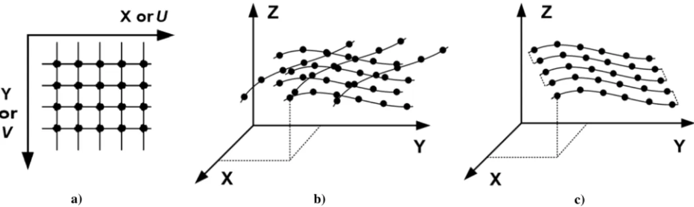
Figure 3. Some topological organizations of 3D data sets, the parameterization of a surface varies according to the scanning method, a) regular grid where a surface is sampled at constant X,Y increments, b) random profiles acquisition from a hand-
held line scanner, c) regular profiles acquisition from a line scanner mounted on a translation stage.
2.2. Parameterization of a 3D surface
The techniques listed above are meant to measure a distance to a point on a scene. It is the scanning mechanism or the projection technique used that define a complete surface s using a surface parameterization given by
T
w
v
u
z
w
v
u
y
w
v
u
x
z
y
x
s
(
,
,
)
=
(
(
,
,
),
(
,
,
),
(
,
,
))
(1)where (u, v) are the variables representing the two degrees of freedom (DoF) of the scanning/projection mechanism (e.g. two deflection angles) and the variable (w) depends on the distance measuring method (angle-derived for triangulation or range for TOF), (x, y, z) are the computed coordinates from both these variables and the parameters extracted after calibration of the laser scanner, and, T is the transpose matrix operator. The rotation matrix and translation vector have been omitted for simplicity but can be important to preserve the 3D data set orientation in space i.e. point of view of the scanner. Other attributes such as color, multi-spectral data or density information have also been removed from the equation for simplicity.
It is important to remember the fact that the surface is not necessarily sampled on a regular (x, y) grid as shown on Figure 3a. Furthermore, uncertainty exists in the resultant spatial coordinates of that surface representation in all three coordinates8. The special case of a sampling regular grid occurs when a triangulation-based probe is mounted on a coordinate measuring machine9. The regular sampling grid is generated by the motion of two orthogonally mounted translation stages that define a Cartesian coordinate system, i.e. s(x,y,z)=(x(u),y(v),z(w))T. In another implementation, intersecting lines (profiles) on the surface can be acquired using a manually operated mechanical arm with appropriate joint encoders or with some optical device that track the profile scanner (Figure 3b).The results are un-organized 3D data sets. With these systems, the sequence does not necessarily follow a spatially continuous acquisition process and therefore the neighborhood information is neither acquired nor kept. A given single profile may contain contiguous sampled points but the surface acquisition will not. These types of 3D data sets are known as un-organized point clouds. The converse exists; if the elements of a 3D data set are topologically organized so that for a given 3D point all the points surrounding it are physically neighbors of that point then, the 3D data set is known as an organized point cloud. The scanning of a surface can be achieved by a profile scanner mounted on a translation rail or rotated with a combination of mechanical devices and mirrors to acquire surface data; here one gets a line by line scanning in a regular fashion (Figure 3c). More recently, flash type 3D imaging devices have appeared on the market. These devices can acquire a full set of organized 3D coordinates of a surface patch simultaneously using a solid-state sensor, a projection lens and a flash source10. Sampling occurs along constant angular increments.
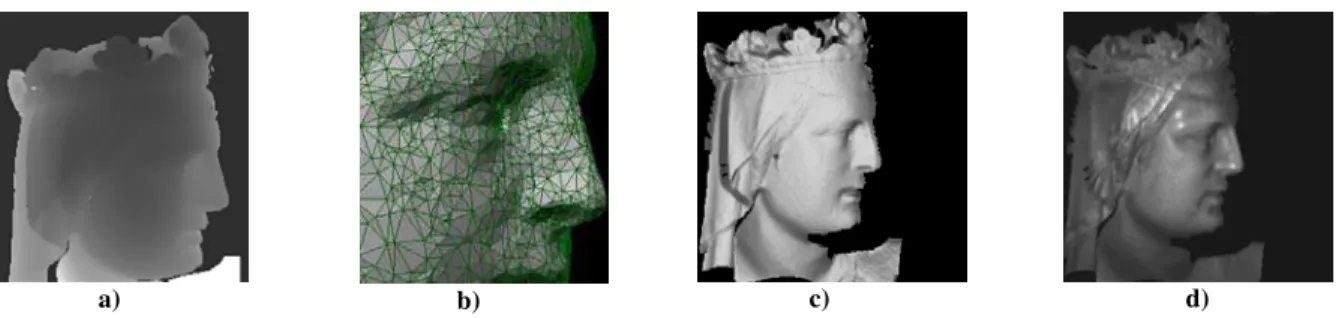
a) b) c) d)
Figure 4. Some representations of an organized point cloud generated from one scan of a portion of a sculpture, a) range coded as a grey scale image (range map), b) wire-mesh showing the connectivity between the 3D points, c) artificial shading of the range map once the 3D points have been organized as a mesh (triangulated), and, d) intensity of the laser return.
2.3. Organized point clouds: 3D surface images
The word imaging implies that the 3D coordinates (more than one) are organized in a particular way. Motion and projection mechanisms have been developed to produce organized clouds of points. The organization of point clouds that take into account the connectivity and neighborhood information between points lends itself to a number of interesting way to process and display 3D information, e.g. simpler calculation of surface normal estimates and mesh creation algorithm. The simplest way of representing and storing surface coordinates of a scene obtained by a sequential acquisition with a uniform (u, v) parameterization (Figure 3a and c) is through the use of a depth or range map (Figure 4a). A depth map is arranged as a matrix where the rows and columns indices are a function of the two orthogonal scan angles (u, v) or some regular interpolated grid in the x and y directions. Continuity information between the points is preserved by the matrix; non valid points are flagged. The matrix cell can contain the corresponding depth measurements (z values), calibrated (x,y,z) values, or any other attribute such as color or uncertainty. In its simplest form, the greyscale image will be composed of ‘depth’ information instead of the intensity information like in Figure 4a. The indices can be the raw scan angles for dual-scan systems, a combination of one scan angle and a translation or other suitable representation describing the surface parameterization from the point of view of the scanner. In some instances, this representation can yield somewhat distorted images. For example, if one flattens a spherically acquired scene using for a hemispherical 3D laser scanner then straight lines will look distorted in a manner similar to panoramic photographic images (see Figure 5).
a) b)
Figure 5. Example of a mid-range laser scanner based on time-of-flight (AM or phase difference) principles that captures 3D coordinates using a spherical laser scanning mechanism: a) laser intensity image generated by laser scanner where the vertical axis depends on the rotating scanning mirror angle and the horizontal axis, on the rotation motor angle, b) same parameterization as in (a) but the distance information is encoded in grey levels (see also Figure 11).
In particular, a triangular mesh can be used to display a range image (see Figure 4b) or using topology dependent slope angles to represent the local surface normal on a given triangle (Figure 4c). The surface normal method yields interesting ways to artificially shade an image in order to highlight and reveal surface details. The object appears to be made of a white material and observed under point source illumination. This representation is used especially to show results obtained from close range 3D systems. It is not always convenient when the 3D data is noisy. One can also display a greyscale value according to either the strength of the laser return signal like in Figure 4d. Finally, other representations and terminology specific to a field exist. Contour and false color maps are also found. The choice of a representation is strongly influenced by the method used to report results for a given application.
Figure 6. Origin of typical uncertainties in Optical 3D imaging systems.
3. ON THE UNCERTAINTIES IN AN OPTICAL 3D IMAGING SYSTEM
The measured coordinates produced by a 3D imaging system need to be completed by a quantitative statement about their uncertainty that is generally based on comparisons with standards traceable to the national units (SI units). Figure 6 summarizes the most important factors that impact on the uncertainty in a 3D imaging system. This diagram is similar to the ISO 14253-2 which provides a list of uncertainty sources11. We will use some parts of this diagram to describe and to quantify uncertainties related to 3D imaging systems. This uncertainty statement is required in order to decide the fitness for purpose of a measurement for a given 3D imaging system (ISO/IEC FDGuide 98-1)12. Mathematical tools and methodologies exist to estimate and report uncertainty, e.g. propagation of uncertainty as described in the ISO Guide to the Expression of Uncertainty in Measurement (GUM). In the field of metrology, the notion of accuracy is considered a qualitative concept and uncertainty is the quantitative statement of accuracy.
3.1. Hardware (HW) means: intrinsic uncertainty of optical distance measurement
El-Hakim and Beraldin summarize the distance or range measurement uncertainty by the standard deviation, δr, for each
class of 3D laser scanners14. The uncertainty of range capture methods can be expressed by a single equation that depends on the signal-to-noise ratio (SNR)15-16 when SNR>10. The range uncertainty has the following form:
SNR K r 1 ≈
δ
(2)where K is a constant dependent on the range capture method. Table 1 lists K as a function of parameters that vary according to the probing method; Z is the distance to a surface, f the collecting lens focal length, B is the baseline between light projector and detector, BW is the root-mean-square signal bandwidth according to Poor’s definition14,Φ is the lens collecting aperture diameter, and λ is laser wavelength, c is the speed of light in vacuum, Tr = rise time of the laser pulse leading edge,λm = wavelength of the amplitude modulation, Δf = tuning range or frequency excursion16,
DOF: Depth of field. The effect of laser speckle is also given along with factors affecting the maximum range that can
be measured with no ambiguity. For very large SNR, triangulation-based methods performance depends on speckle noise. For time delay-based systems, speckle will affect the amplitude of the returned signal. The SNR depends among other things on the light source power, detector sensitivity, distance to a surface, the type of surface (opaque, Lambertian, specular, retro-reflective, curvature, translucency, etc..), the collection lens size. With coherent detection, the SNR is limited by the shot-noise-limited condition that is achieved by increasing the optical power of the reference signal. Relatively low range uncertainties can be obtained by a large frequency excursion possible by the modulation of the optical frequency e.g. 100 GHz.
Other systems level performance in terms of spatial resolution, surface sampling intervals and speed characterize 3D systems. Many references address the limits imposed by diffraction on the resolving power along the X and Y-axes (lateral optical resolution) of 3D laser systems2,14,29. Usually a surface cannot be sampled at equidistant spatial intervals because of the scanning method. The collection of light rays and the surface topology also prevent that. It is only in rare cases that an equidistant sampling can be achieved. For instance, a triangulation-based 3D system is normally composed of a light projector (laser or white light), a collecting lens and photo-sensor (linear or matrix arrays). Hence, the 3D imaging system acquires information also along radial lines that diverge to a surface and reconverge from a surface back to a collecting lens onto a photo-sensor. This projective optics characteristic will shape the sampling of the 3D surface being sampled.
Table 1. Range uncertainty as a function of SNR and speckle noise,
Method Constant K Speckle noise δr Max range Typical values
Triangulation BW B f Z2 1 Φ B Z2 2 π λ Limited by the optical geometry 0.02 mm - 2 mm DOF < 4 m @ 10 - 1000 kHz PW modulation Tr c 2
Affects amplitude Limited by pulse rate fp 5 mm - 50 mm DOF > 10 m @ 1 - 250 kHz AM modulation π λ 4
m Affects amplitude Limited by
frequency fm 0.05 mm - 5 mm DOF 1-100 m @ 50- 1000 kHz FM modulation f c Δ π 2
3 Affects amplitude Limited by
chirp duration Tm
0.01 to 0.25 mm DOF < 10 m @ 0.01-1 kHz
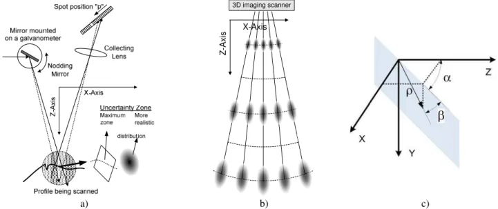
Figure 7a illustrates this characteristic for the case of a triangulation laser spot scanner. Considering that a mirror scans the laser beam with a certain error and that the spot position is also measured with some error, then the 3D location on a surface will be bounded in a region (rhombus). The rhombus delimits a maximum zone of error or uncertainty zone. A more detailed analysis can yield the probability density of the measurement error by using the uncertainties of the scanning mechanism and the distance measurement method (Table 1). This is shown schematically on Figure 7b. It represents the measurement uncertainty for a laser spot scanner as the object moves away from the camera: the sampling interval increases and the size of the distribution of the error (δr) around a given position also increases.
3D imaging scanner
Z-Axis
X-Axis
a) b) c)
Figure 7. Error distribution: a) for a triangulation-based laser spot scanner; zone of uncertainty caused by the sampling interval of the mirror scanner and of the laser spot position sensor, b) more realistic estimate of the shape of the measurement uncertainty within the whole field of view of a laser spot scanner and c) coordinate system for a monostatic TOF system.
The error (δr) is a function of not only the intrinsic uncertainty for a given 3D method (Table 1) but also of quantization
noise, systematic biases due to calibration errors, noise from surface roughness or the effects due to the propagation medium. For example, Hebert et. al.8 use a detailed sensor model to extract lines from scattered 3D data. Boulanger17 use Gaussian error distribution and error propagation law to model sensor error for intrinsic filtering of 3D images. One can determine from the range equations of a monostatic TOF systems, the expected uncertainty along the x y z directions. With reference to Figure 7c, the range equations are as follows
)
cos(
)
cos(
)
sin(
)
cos(
)
cos(
α
β
ρ
β
ρ
α
β
ρ
=
=
=
z
y
x
(3)Excluding the correlation terms and assuming that the variance of the pointing error of the laser beam for a monostatic TOF systems18 is given by (δα)2 in both scan axes and that the range error variance is (δρ)2 then the diagonal terms of the
covariance matrix for a point (x, y, z) is given by
)
,
,
(
)
(
p
diag
ρ
2δ
α2ρ
2δ
α2δ
ρ2V
≈
(4)For instance, let us consider a system that measure at ρ= 5 m, δρ= 1 mm and δα = 20 µrad then (δx ,δy ,δz) = (0.1 mm,
0.1 mm, 1 mm). One should remember that the underlying hypothesis of active optical geometric measurements is that the imaged surface is opaque and diffusely reflecting. It is not the case of all materials. Problems arise when trying to measure glass, plastics, machined metals (with striations), or marble19. For marble, the range uncertainty with a 3D laser triangulation system varies with the spot dimension and a systematic bias appears in the surface location measurement. For a time-of-flight based 3D system an apparent systematic bias in distance measurement appears20. Additionally, the
type of feature being measured is an important factor affecting the performance of a 3D imaging system. Systematic errors of active 3D cameras increase when measurements are performed on objects with sharp discontinuities such as edges and holes or when high contrast surfaces are measured21-23.
3.2. Hardware (HW) means: acquiring full surface data & surface parameterization
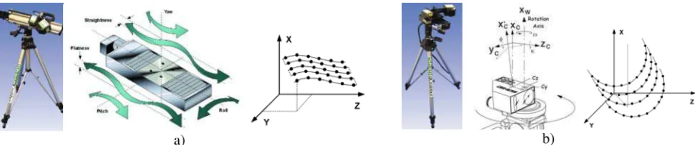
The acquisition of full 3D surface data can be accomplished in a number of ways depending on the principle used to measure 3D shape and projection/scanning mechanism used. Beraldin 2007 lists a number of methods to acquire full surface data using structured light (active methods). These cover scanning mirrors/motors, optical/mechanical tracking devices or solid state devices. Motorized translation and rotation stages may become the limiting factor in portable 3D imaging systems (see Figure 8). In order to obtain low uncertainties and straightforward calibrations, a number of errors need to be estimated and compensated. These include cosine errors, straightness, flatness, pitch/roll/ yaw wander and wobble, motion hysteresis and backlash, and, encoder errors. If loads (3D imaging system or work piece) are not properly mounted then sag due to flexure and torsion may occur. If not compensated, these errors will show up when multiple scans are merged together to form a 3D model or in single 3D image applications, these errors may produce a false reject of a work piece.
a) b)
Figure 8. Motion stage errors and intrinsic parameterization: a) 3D camera based on a sheet of light mounted on a motorized translation stage, errors originating from a linear translation stage, and its parameterization, b) 3D camera based on a sheet of light mounted on a motorized rotation stage, errors originating from that rotation stage, and its parameterization.
Any metallic structure will change shape according to temperature and load characteristics. We summarize the calculations of the effect of flexure and torsion on a linear translation stage. An analysis of this set-up reveals that the sag due to both effects is approximately given by
L
J
G
A
L
A
e
g
M
L
I
E
A
L
A
g
M
t t f s)
(
3
)
(
2 3 3 3−
+
−
=
Δ
+
Δ
=
Δ
(5)Referring to Figure 9, we assume the length L=1000 mm, the distance et=100 mm, the mass of the camera-carriage M=4
kg, the modulus of elasticity of the steel Z30-C-13 used is E=200 000 N/mm2, the shear modulus G=75 000 N/mm2, moment of inertia (Flexure) I=24 000 mm2, the polar moment of inertia (Torsion) J=16 700 mm2, the dimensions of the cruciform rail are wh=10 mm; wv=10 mm; h=30 mm. For this particular case, the sag due to flexure will be the largest in the middle of the rail, i.e., about 42 µm while the torsion about 78 µm. A reduction of the rail length to 600 mm and the load weight to 3 kg will give 7 µm and 35 µm for flexure and torsion respectively. A triangulation-based system with the following characteristics (λ=0.632 µm, B=150 mm, Z=300 mm, Φ=20 mm, speckle noise-limited – see Table 1) can
potentially yield a theoretical distance uncertainty of 4.3 µm. This estimate of the uncertainty (random part) is within the range calculated for the systematic error. For that system and using the last example then, the torsion-related systematic error should be removed through an adequate calibration.
Figure 9. Flexure and torsion on a translation stage under realistic loading: left diagram represents the frontal view of a system where the 3D profile camera is mounted on a rectilinear translation stage, center diagram shows a side view of the camera as mounted on a motorized carriage, right diagram show details of the cross-section of the rail (cruciform).
3.3. Software (SW) means: Analytical tools for geometric fitting
Here, we limit the topic on the impact of software tools on system uncertainty to the geometric fitting of surfaces. Geometrical artifacts (objects) like flat planes, spheres, cylinders, and cubes allow a user an easy way to test a 3D imaging system. They can be purchased at a reasonable cost and they can be accompanied by a certificate. Though these objects provide us with surfaces that go from flat to curved, the simple to the combined arrangements or the mat finish to the specular one, they are not always best for testing a system under real conditions. They provide us only with a common way to compare systems. Figure 1 gives some objects that were used in the section on experiments. More complex objects (e.g. freeform) have been fabricated and characterized but are beyond the scope of this paper. In order to estimate the performance of a given system using the geometric feature of an object, one has to compare it with the expected surface, e.g. flat surface measured should be flat up to a certain level of errors (random and systematic). The estimation of a surface requires an excellent knowledge of parameter estimation of geometric models from noisy data25. The general problem of fitting can be stated as follows: fit a geometric model of a surface using an implicit equation:
0
)
;
(
p
u
=
F
(6)to N 3D data points pi, i=1,…,N; the vector u contains the parameters of the geometric model. Each 3D data point is
perturbed by noise from its true value pi which satisfies (6). The random noise is in many cases described by a Gaussian random variable. Caution should be exercised because the noise along the (x, y, z) axes is correlated, anisotropic and inhomogeneous8,17 (see section 3.1). A good estimator ( uˆ ) of the parameter u from the observed data pi is required.
Good in the sense that its covariance matrix [ uˆ ] is small. Many algorithms exist to minimize this covariance matrix. Kanatani lists and explains the most common ones found in the scientific literature25. Estimators need to be unbiased and consistent. As noted by Kanatani, in some situations “the removal of systematic errors and outlying data is more important than optimal estimation on the Gaussian noise assumption”.
V
In the experimental section, we use a flat plane with a given reflectance to estimate the errors (random and systematic) along the range and for different reflectance values. Spheres are used to understand the errors in estimating the diameter and the form error. Unfortunately, if one uses a commercial analysis package, it is not clear what the underlying algorithms for fitting are. From statistics and under certain circumstances, it is expected that the standard deviation of the parameters of the plane after fitting will be proportional to the noise level and inversely proportional to N; the standard deviation of the normal to the plane will be proportional to the noise level and inversely proportional to both N and Extentof the plane (see Figure 10). The estimate of the sphere radius (expected value) will be biased by the noise variance divided by the actual sphere radius.
a) b)
Figure 10. Simple geometric objects used in the experiments: a) flat surface specified by the material (e.g. vapour blasted Aluminum), flatness (better than the random noise of DUT) and b) sphere with known radius and cooperative surface reflectance.
4. EXPERIMENTAL RESULTS
Theoretical considerations can enlighten us on some aspects of a measurement device. Experimentations, on the other hand, can be tailored to estimating a certain aspect of a system without performing long mathematical derivations. From the uncertainty analysis of section 3.1, one can conclude that 3D artifacts will need to have different surface reflectivity, form factor and finish. They will need to be located at known distances and orientations. Their physical dimensions will depend on the system’s measurement principle and the practicality of the situation. An object that is distinct from the calibration equipment and for which the accuracy is 4-5 times (rule of thumb) better than that of the range camera is employed in such an evaluation. For instance, a scale bar made of a stable material with low thermal coefficient of expansion (TCE), e.g., SuperInvar, Invar (TCE~2 ppm/oC) or composite materials, can be used as a compact traveling standard. Other objects with known features and surfaces can be manufactured from stable materials and measured with instruments that have tight tolerances compared to the DUT (Device Under Test). The cost of test objects depends on the material used as well as the care that was put in their construction and certification. Furthermore, the algorithms applied to the raw range measurements obtained from the 3D imaging system will have an impact on the uncertainty attached to the whole measurement chain. Therefore, the evaluation methods along with definitions of terms are fundamental for metrology research and standards2,11,12,26,27.
a) b) c)
Figure 11. Set-up used to evaluate local range uncertainty: a) Surphaser® in an environmentally controlled laboratory at NRC-IIT (20.0 ± 0.1°C, RH=50% ± 5%), b) HDS600® at The Helsinki University of Technology (TKK), Department of Surveying,
c) CallidusCPW 8000 ® at the same University (20 ± 2°C, RH=unknown).
4.1. Estimation of uncertainty: random component on flat targets and a greyscale target
We report the standard deviation of a best plane fit on the X95 end-plate and on the reflectance scale (see Figure 12). The results were obtained from the software PolyWorks/IMInspect™ v10. The algorithm is not known to the author but it performs a best fit with outlier removal. For the reflectance target, small patches were selected as the flatness is not well controlled for that particular target. Table 2 presents the results. The three scanners shown on Figure 11 were used for the tests. The angular sampling was set at the highest recommended by the manufacturer, i.e. for the Surphaser and HDS 6000, 0.009 degrees in both scan axes and 0.02 degrees for the Callidus CPW8000.
a) b)
Figure 12. Artifacts used to quantify the range uncertainty (random) as a function of distance and reflectance: a) vapor-blasted X95 structural rail end-plate from Newport, b) opaque target glued on a flat mirror. From the calibration certificate, the response is flat from 450 nm out to 750 nm (89.2%, 19.2%, 9.3%, 3.1%).
One can see the effect of a decreasing SNR as the distance increases and the reflectance is lowered. Two scanners (Surphaser and Callidus) did not return data for the reflectance patch at 3%. The HDS6000 returned 3D data for that reflectance patch but the standard deviation is substantially larger than what was found for the other reflectance patches. The HDS 6000 had a laser power level setting that the others did not have. We used the high power mode.
Table 2. Estimated uncertainty (mm) on a flat object and a greyscale object at different distances (ρ) to a scanner. SPS:
Surphaser ®, HDS: HDS6000®, Cal: CallidusCPW 8000 ®. The reflectance value (R) has an error of about ±0.25 % (calibration certificate and angle of plate wrt line of sight). Na: Not available.
SPS HDS Cal ρ R 2950 mm 4950 mm 8940 mm 3380 mm 6860 mm 10060 mm 14000 mm 3280 mm 10950 mm 89 % 0.15 0.15 0.16 0.51 0.48 0.56 0.75 1.0 1.36 19 % 0.29 0.28 0.33 1.1 1.04 1.22 1.77 1.33 2.22 9 % 0.46 0.49 0.56 1.73 1.55 2.02 2.46 1.64 2.36 3 % Na Na Na 3.5 2.91 3.54 5.76 2.75 Na a) b) c)
Figure 13. Systematic errors caused by a translation rail: a) solid block of Amersil T08 fused quartz lapped flat to < 0.002 mm, b) error map after fitting a plane trough the 3D image generated by a 3D laser camera mounted horizontally, c) same as (b) but the 3D laser camera is mounted looking down on the flat plane (top of color scale 0.25 mm and bottom of scale -0.05 mm).
4.2. Estimation of uncertainty: systematic bias on a flat surface and a greyscale target
A flat surface made of a solid block of Amersil T08 fused quartz of dimensions 300 mm×50 mm×50 mm with all sides ground square and parallel to 0.005 mm with one face lapped flat to < 0.002 mm with a grit size of 0.005 mm was used to evaluate the systematic errors due to torsion and flexure on a camera mounted on a translation stage (ShapeGrabber®102). The lapped surface is coated with a vacuum deposited opaque layer of chromium. This type of artifact can also be used to measure the quality parameter flatness according to VDI/VDE 263426. This surface was measured with the system shown in Figure 8a. The stage was oriented in two directions: 1) camera moving horizontally in a well balanced manner and 2) with the camera pointing down towards the object. The 3D laser camera has an estimated uncertainty (random 1 sigma) of about 0.01-0.02 mm at close range. The translation stage can move the 3D
laser camera by 300 mm. In the first position, the systematic error is within ± 0.025 mm which is perceptible (Figure 13b) but for a smaller scan length can be neglected. In the second position, the flexure and tensional errors are really visible. The error varies between -0.05 mm and +0.25mm! If the systematic behavior cannot be calibrated out of the system, one must change the motion stage or perform very small displacements. These systematic errors are larger than what was estimated in section 3.2. This is due to a totally different mechanical structure in the actual translation stage. The technical specifications were not available to the author during this study.
It has been observed by some authors that TOF systems may produce a bias in the range data when two surfaces with different reflectance are measured at the same location21,23. We conducted an experiment using the object shown on Figure 12b and three TOF-AM modulation systems. We first made sure there was no penetration of the laser onto the target. This was tested with two close range laser scanners. Plane equations are fitted using the same method discussed above. We report some results on Figure 14. It was found that the Surphaser® scanner gave a bias of 0.5 mm at the highest reflectance (89%) and at the closest distance tested (2950 mm from the scanner). At the other distances, the bias is lower than 0.1 mm. The Callidus CPW-8000® scanner yielded a bias of 3.3 mm at the lowest reflectance (3%) and at 3280 mm from the scanner; no data is available at 10950 mm. The HDS 6000® gave no measurable bias.
a) b) c)
Figure 14. Profile of the point clouds on the reflectance chart: a) Surphaser®, b) HDS6000®, c) CPW8000®. Not to scale!
5. CONCLUSION
This paper reviewed some basic principles of 3D imaging systems, i.e., optical triangulation and time delay (time-of-flight) measurement systems. The intrinsic uncertainty of optical distance measurement techniques, the parameterization of a 3D surface and systematic errors were reviewed. These basic concepts should guide the reader in understanding surface measurement uncertainty of 3D imaging systems and allow devising a methodology and a set of artifacts that can be used for the evaluation of the performance of a given system. Experimental data were also provided to support the theoretical presentation. Commercially available scanners were tested in controlled and semi-controlled environments. Some results can be explained only if the manufacturers of the scanners and the software release detailed information about their products. We don’t see this as a feasible solution in the near future and hence a standards need to be created (terminology, test methods, etc…) as soon as possible. Such a standard will have to address the aspects presented in this paper as well as many more quality parameters like distance accuracy, lateral resolution, dynamic range etc. Furthermore, all the tests should at least contain the following information for each quality parameter: the artifact with its form & reflectance certification, the procedure, the evaluation method and the assessment of the result.
ACKNOWLEDGEMENTS
The author acknowledges the various collaborators that have participated in the realization of the tests discussed in this paper. Many thanks go to the team (N. Heiska, A. Erving, M. Nuikka, H. Haggren) at The Helsinki University of Technology (TKK), Department of Surveying that organized the demonstrations with the Leica HDS6000® and Callidus CPW8000®. The author wants to acknowledge also the help of Luc Cournoyer and Michel Picard from NRC for the acquisition of the 3D images. Innovmetric Software Inc. Canada supplied the evaluation software.
REFERENCES
[1] Blais, F., "A review of 20 years of range sensor development," Journal of Elect. Imaging, 13(1), 231-243, (2004). [2] Cheok, G. S., Lytle, A. M., Saidi, K. S., "Standards for 3D imaging systems," Quality Design, July, pp.35-37 (2008). [3] Pfeifer, N. and Briese, C., "Geometrical aspects of airborne laser scanning and terrestrial laser scanning," IAPRS
Volume XXXVI, Part 3/W52, pp. 311-319, (2007).
[4] Beraldin, J.-A., Blais, F., Lohr, U., "3D Imaging laser scanners technology", Chap. 1, in Airborne and terrestrial laser scanners, G. Vosselman and Hans-Gerd Maas editors, Whittles Publishing, UK, (2009). In press.
[5] Jahne, B., Haußecker, H., Geißler, P., Handbook of Computer Vision and Applications, Academic Press, San Diego, Volume 1: Sensors and Imaging, Chap. 17-21, (1999).
[6] Seitz, P., "Photon-noise limited distance resolution of optical metrology methods," Proceedings of SPIE Volume 6616 Optical Measurement Systems for Industrial Inspection V, Wolfgang Osten, Christophe Gorecki, Erik L. Novak, Editors, 66160D. Jun. 18, (2007).
[7] Donati, S., Electro-Optical Instrumentation: Sensing and Measuring with Lasers, Prentice Hall, (2004).
[8] Hébert. P., Laurendeau, D., Bergevin, R., "From 3-D scattered data to geometric signal description: invariant stable recovery of straight line segments," Int. J. Pattern Recogn. Artif. Intell. Vol.8, No.6, pp. 1319-1342, (1994).
[9] Fan, K.-C., "A non-contact automatic measurement for free-form surface profiles," Computer integrated Manufacturing systems, 10(4), pp. 277- 285, (1997).
[10] Hosticka, B., Seitz, P., and Simoni, A., "Optical Time-of-Flight Sensors for Solid-State 3D-Vision, " Encyclopedia of sensors, Edited by C.A. Grimes, E.C. Dickey, and M.V. Pishko, Vol 7, pp. 259-289, (2006).
[11] ISO/TC 14253-2, “Guide to the estimation of uncertainty in Geometrical Product Specifications (GPS) measurement, in calibration of measuring equipment and in product verification,” (1999).
[12] ISO/IEC Guide 98-3:2008, Uncertainty of measurement – Part 3: Guide to the expression of uncertainty in measurement (GUM:1995), (2008).
[13] Taylor, B. N., Kuyatt, C. E., "Guidelines for Evaluating and Expressing the Uncertainty of NIST Measurement Results," NIST Technical Note 1297, 1994 Edition, United States Department of Commerce, Technology Administration National Institute of Standards and Technology, 26 pages, (1994).
[14] El-Hakim, S. F., Beraldin, J.-A., "Sensor Integration and Visualisation," Chap.10 in "Applications of 3D Measurements from Images" edited by J. Fryer, A. Mitchell and J. Chandler, Whittles Publishing, UK, (2007). [15] Poor, H.V., An introduction to signal detection and estimation. 2nd Ed., NY: Springer-Verlag.p. 331, (1994). [16] Skolnik, M.L., Introduction to radar systems, McGraw-Hill Company, NY, USA, 2nd Ed., (1980).
[17] Boulanger, P., Jokinen, O., Beraldin, J.-A., "Intrinsic Filtering of Range Images Using a Physically Based Noise Model," The 15th International Conference on Vision Interface, Calgary, Canada, 320-330, May 27-29, (2002). [18] Bae, K., Belton, D., Lichti, D., "A Closed-Form Expression of the Positional Uncertainty for 3D Point Clouds,"
IEEE Transactions on Pattern Analysis and Machine Intelligence, Forthcoming, (2008).
[19] Godin, G., Rioux, M., Beraldin, J.-A., Levoy, M., Cournoyer, L., Blais, F., "An assessment of laser range measurement on marble surfaces," 5th Conf. on Opt. 3D Meas. Techniques, Wien, Austria, Oct. 1-4, 49-56, (2001). [20] El-Hakim, S. F., Beraldin, J.-A., Picard, M., Cournoyer, L., "Surface Reconstruction of Large Complex Structures
from Mixed Range Data - The Erechtheion Experience," The XXI Congress of the International Society for Photogrammetry and Remote Sensing (ISPRS 2008). July 3, (2008).
[21] Boehler, W., Bordas, M., Marbs, A., "Investigating laser scanner accuracy, " Proc. CIPA XIXth Int. Symposium, 30 Sept. -4 Oct., Antalya, Turkey, pp. 696-702, (2003).
[22] Blais, F., Taylor, J., Cournoyer, L., Picard, M., Borgeat, L., Dicaire, L.-G., Rioux, M., Beraldin, J.-A., Godin, G., Lahanier, C., Aitken, G.,"Ultra-High Resolution Imaging at 50µm using a Portable XYZ-RGB Color Laser Scanner," Intern.W. on Recording, Mod. and Vis. of Cultural Heritage. Ascona, Switzerland. May 22-27, (2005). [23] Clark, J., Robson, S., "Accuracy of Measurements Made with a Cyrax 2500 Laser Scanner Against Surfaces of
Known Colour, " ISPRS XX Congress-Commision 4, pp. 1031-1036, (2004).
[24] Beraldin, J.-A., Rioux, M., Cournoyer, L., Blais, F., Picard, M., Pekelsky, J., "Traceable 3D Imaging Metrology," The Symposium: Annual IS&T/SPIE on Electronic Imaging. Videometrics IX (E1103). San Jose, California, USA. Jan. 28 – Feb. 1, (2007).
[25] Kanatani, K., "Statistical Optimization for Geometric Fitting: Theoretical Accuracy Bound and High Order Error Analysis, " International Journal of Computer Vision, 80(2), pp.167-188, (2008).
[26] VDI/VDE 2634 Blatt 2, Optische 3D-Messsysteme - Systeme mit flachenhafter Antastung/Optical 3-D measuring systems - Optical systems based on area scanning, 11 pages, Aug. (2002). Blatt 3, Optische 3D-Messsysteme - Bildgebende Systeme mit flächenhafter Antastung in mehreren Einzelansichten/Optical 3D-measuring systems - Multiple view systems based on area scanning, Sept. (2006).
[27] ISO VIM (DGUIDE 99999.2), International Vocabulary of Basic and general terms in metrology (VIM) – Third edition, (2006).
[28] Committee E57 on 3D Imaging Systems, ASTM International. http://www.astm.org/cgi-bin/SoftCart.exe/COMMIT/COMMITTEE/E57.htm?L+mystore+ftmy6332 last accessed 1 November 2008. [29] Khoury, J., Woods, C. L., Lorenzo, J., Kierstead, J., Pyburn, D., Sengupta, S. K., "Resolution limits in imaging ladar