Bayesian Scene Understanding with Object-Based
Latent Representation and Multi-Modal Sensor
Fusion
by
Michael A. Wallace
S.B., Massachusetts Institute of Technology (2017)
Submitted to the Department of Electrical Engineering and Computer
Science
in partial fulfillment of the requirements for the degree of
Master of Engineering in Electrical Engineering and Computer Science
at the
MASSACHUSETTS INSTITUTE OF TECHNOLOGY
February 2021
© Massachusetts Institute of Technology 2021. All rights reserved.
Author . . . .
Department of Electrical Engineering and Computer Science
December 9, 2020
Certified by. . . .
John W. Fisher III
Senior Research Scientist
Thesis Supervisor
Accepted by . . . .
Katrina LaCurts
Chair, Master of Engineering Thesis Committee
Bayesian Scene Understanding with Object-Based Latent
Representation and Multi-Modal Sensor Fusion
by
Michael A. Wallace
Submitted to the Department of Electrical Engineering and Computer Science on December 9, 2020, in partial fulfillment of the
requirements for the degree of
Master of Engineering in Electrical Engineering and Computer Science
Abstract
Scene understanding systems transform observations of an environment into a rep-resentation that facilitates reasoning over that environment. In this context, many reasoning tasks benefit from a high-level, object-based scene representation; quan-tification of uncertainty; and multi-modal sensor fusion. Here, we present a method for scene understanding that achieves all three of these desiderata. First, we in-troduce a generative probabilistic model that couples an object-based latent scene representation with multiple observations of different modalities. We then provide an inference procedure that draws samples from the posterior distribution over scene representations given observations and their associated camera parameters. Finally, we demonstrate that this method recovers accurate, object-based representations of scenes, and provides uncertainty quantification at a high level of abstraction.
Thesis Supervisor: John W. Fisher III Title: Senior Research Scientist
Contents
1 Introduction 7
1.1 Object-Based Scene Representation . . . 8
1.2 Uncertainty Quantification . . . 9
1.3 Multi-Modal Sensor Fusion . . . 9
1.4 Outline . . . 10
2 Background 11 2.1 Sampling-Based Inference . . . 11
2.1.1 Metropolis-Hastings . . . 12
2.1.2 Gibbs Sampling . . . 12
2.1.3 Reversible-Jump Markov Chain Monte Carlo . . . 13
2.2 Camera Models . . . 14 2.2.1 Extrinsics . . . 15 2.2.2 Intrinsics . . . 16 2.3 Analysis by Synthesis . . . 17 2.4 Related Work . . . 17 2.4.1 Sampling-Based Inference . . . 17 2.4.2 Amorized Inference . . . 19 3 Model 21 3.1 Scene . . . 23 3.1.1 Model . . . 23 3.1.2 Parameterization . . . 24
3.1.3 Prior . . . 26 3.2 Sensors . . . 27 3.2.1 Extrinsics . . . 27 3.2.2 Intrinsics . . . 28 3.2.3 Prior . . . 29 3.3 Observations . . . 29 3.3.1 Rendering Function . . . 31 3.3.2 Image Likelihood . . . 32 3.3.3 Depth Likelihood . . . 32 3.4 Discussion . . . 32 4 Inference 35 4.1 Sampling Scene . . . 36
4.1.1 Sampling Object Parameters . . . 38
4.1.2 Sampling Scene Model . . . 41
4.2 Sampling Noise Parameters . . . 49
4.3 Discussion . . . 50 5 Results 53 5.1 Single-Object Scene . . . 54 5.1.1 Sampling . . . 55 5.1.2 MAP Estimates . . . 58 5.1.3 Uncertainty Quantification . . . 60 5.1.4 Proposal Acceptance . . . 62 5.2 Multi-Object Scene . . . 64 5.2.1 Single Camera . . . 66 5.2.2 Multiple Cameras . . . 68 5.3 Discussion . . . 70 6 Conclusion 71
Chapter 1
Introduction
Scene understanding involves tranforming one or more observations of a scene into some representation that is useful for downstream tasks. Such transformations are applicable whenever autonomous agents must reason about their environment in order to operate (e.g., robotic disaster response [21, 24], autonomous driving [3, 4, 10]), as well as when automated systems structure or summarize sensory input to assist human activities (e.g., assistive techology [17, 25], surveillance [18, 19]).
Scene understanding is a broad problem, and many approaches have been pro-posed to solve its variants. Here, we focus our attention on scene understanding for applications where the following (motivated in subsequent sections) are desired:
1. an object-based scene representation, where a scene is expressed as a collection of objects, each with parameters that correspond to absolute, world-centric (not observation-centric) object properties (Section 1.1);
2. uncertainty quantification, at the level of the object-based scene representation (Section 1.2);
3. multi-modal sensor fusion, or the ability to integrate disparate sources of infor-mation from multiple sensing modalities (Section 1.3).
In this thesis we propose a novel scene understanding method that – to the best of our knowledge – is the first to achieve all three of these desiderata. The primary
goal of this thesis is to present and examine an approach that incorporates all of the elements noted above with particular emphasis on reasoning
1.1
Object-Based Scene Representation
In this thesis we use an object-based scene representation, where a scene is a collec-tion of objects, each with associated parameters. The parameterizacollec-tion of objects may vary between different types of objects, depending on the relevance of different parameters to each type. We do not make the argument that an object-based rep-resentation is optimal – this ought to depend type of scene being modeled and the downstream tasks being supported – nor that it is novel [7, 8, 15], but that it has several appealing properties that motivate its use.
First, this representation is expressive and general-purpose. Like many common scene representations (e.g., voxels, point-cloud, mesh), an object-based representation is flexible enough to represent almost any scene. Furthermore, it is able to support a wide range of downstream tasks, in contrast to representations that were learned for a particular task. Second, this representation is three-dimensional. While two-dimensional representations (e.g., bounding boxes, pixel segmentation) have proven useful, many practical tasks require reasoning about a scene in three dimensions and it is useful to have a representation that directly supports this. Third, an object-based representation directly supports many high-level reasoning tasks. For example, with this representation it is straightforward for an autonomous agent to reason over whether the tools required to complete some task are present and how it should best retrieve them. Finally, this representation is highly interpretable, making it more suitable for human-in-the-loop applications than abstract representations, such as those learned in autoencoder methods.
1.2
Uncertainty Quantification
Uncertainty is inherent in scene understanding problems. This includes both alleatoric uncertainty (e.g., sensor noise) as well as epistemic uncertainty (e.g., unobserved parts of the scene). In many applications, quantifying uncertainty about the scene is helpful for downstream tasks. For example, an autonomous agent can avoid taking a path through an uncertain part of the scene. In some applications (e.g., autonomous driving), uncertainty quantification is safety-critical [1].
Often, scene understanding methods that incorporate uncertainty quantification do so over low-level geometric primitives (e.g., voxels, mesh) [5, 6]. On the other hand, the inference procedure we describe yields a distribution over the nonparametric, object-based latent representation. While all of these methods permit uncertainty quantification at a low level of abstraction (e.g., which parts of the scene are occupied), the object-based representation also permits higher-level uncertainty quantification (e.g., how many objects are in the scene). We demonstrate both of these capabilities in Chapter 5, and note that this is by no means exhaustive.
1.3
Multi-Modal Sensor Fusion
In practical applications, no single observation provides enough information for a complete understanding of the scene. This could be due to observations originating from different viewpoints, or observations coming from different sensing modalities that provide complementary information about the scene. In these cases, it is neces-sary to fuse information from multiple observations into a unified understanding of the scene.
The probabilistic model we describe combines both RGB and depth camera ob-servations with arbitrary intrinsics and extrinsics. Notably, inference does not rely on prior training with a particular sensor configuration. Also of note, is that this method directly couples the object-based latent representation and raw sensor infor-mation with no semantic interpretation, respecting the physics of the sensing process.
1.4
Outline
At a high level, in Chapter 3 we present a generative model for scenes and observa-tions, in Chapter 4 we describe an inference procedure to estimate the posterior over scenes given observations, and in Chapter 5 we demonstrate the inference procedure using synthetic scenes.
In Chapter 3, we present a probabilistic model that couples an object-based la-tent representation with multiple observations from both RGB and depth cameras. In this model, we describe a scene as a collection of objects, each with a parameter-ization according to its object class. We also show how to evaluate the likelihood of scenes using this representation under RGB and depth observations, using analysis by synthesis [2] (Section 2.3).
In Chapter 4, we describe a sampling-based inference procedure to approximate the posterior distribution over our nonparametric object-based latent space, given the observations. This approach allows us to not only obtain point estimates of the objects in scenes and their parameters, but to quantify uncertainty about our understanding of a scene at the object level.
Finally, in Chapter 5, we demonstrate inference using synthesized scenes and ob-servations. We show that inference recovers accurate object-based scene representa-tions, including in situations where information is distributed across multiple sensors and any single-sensor method would fail to produce a complete understanding of the scene. We also show that samples obtained from the inference procedure permit both low-level and high-level uncertainty quantification.
Chapter 2
Background
In this thesis, we draw on sampling-based inference (Section 2.1) to estimate the posterior over scene representations given observations. In order to evaluate the likelihood, we use perspective camera models (Section 2.2) and analysis-by-synthesis (Section 2.3). In this Chapter, we outline the basics of these models and techniques, and provide references to further information.
In Section 2.4, we also outline related work in scene understanding.
2.1
Sampling-Based Inference
For most complex probabilistic models, exact probabilistic inference is intractable. In many cases, sampling-based inference provides a tractable alternative to estimate statistics over a distribution.
Sampling-based inference methods, as their name suggests, draw samples from some distribution 𝑝(𝑥). With a large enough number of samples, computing statis-tics of 𝑝(𝑥) is well approximated by computing empirical expectations over samples {𝑥𝑡}𝑇𝑡=1, 1 𝑁 𝑇 ∑︁ 𝑡=1 𝑓 (𝑥𝑡) → ∫︁ 𝑥 𝑓 (𝑥)𝑝(𝑥) d𝑥 = E𝑝[𝑓 (𝑥)] ,
by the strong law of large numbers. Similarly, the mode of the distribution can be estimated by taking the maximum a posteriori (MAP) sample.
Though efficient methods exist for drawing samples from simple distributions, drawing samples from more complex distributions (such as those dealt with in this work) is not so straightforward. Robert and Casella [23] provide a thorough treatment of the many sampling-based inference methods. Here we review three algorithms used in this work: Metropolis-Hastings, Gibbs sampling and Reversible-Jump Markov chain Monte Carlo.
2.1.1
Metropolis-Hastings
In order to draw samples from 𝑝(𝑥), the Metropolis-Hastings algorithm constructs a Markov chain over the support of 𝑝(𝑥) that is ergodic and has 𝑝(𝑥) as the stationary distribution [14]. By constructing the Markov chain in this way, samples from the chain converge to samples from 𝑝(𝑥). It suffices to be able to evaluate 𝑝′(𝑥) ∝ 𝑝(𝑥) to construct such a Markov chain. From state 𝑥, the algorithm proceeds by proposing a new state 𝑥′ using any distribution 𝑞(𝑥′|𝑥) that assigns nonzero probability to the support of 𝑝(𝑥), and accepting a transition to the proposed state with probability
𝐴(𝑥′, 𝑥) = min (︂ 1, 𝑝 ′(𝑥) 𝑝′(𝑥′) · 𝑞(𝑥 | 𝑥′) 𝑞(𝑥′ | 𝑥) )︂ . This quantity is known as the acceptance probability, with the ratio
𝑝′(𝑥) 𝑝′(𝑥′)·
𝑞(𝑥 | 𝑥′) 𝑞(𝑥′ | 𝑥)
known as the Hastings ratio. Choosing to accept or reject sample proposals using this acceptance probability ensures detailed balance, as described in Chapter 6 of Robert and Casella [23]. This is sufficient to guarantee that sampling the Markov chain will converge to sampling 𝑝(𝑥), given enough samples.
2.1.2
Gibbs Sampling
Given a multivariate distribution 𝑝(𝑥) where 𝑥 can be partitioned into {𝑥𝑖}, Gibbs
by sampling from the full conditional 𝑝(𝑥𝑖 | 𝑥−𝑖) [11]. So long as each variable set 𝑥𝑖
is sampled infinitely often, this Markov chain has stationary distribution equal to the joint 𝑝(𝑥).
In contrast to the more general Metropolis-Hastings algorithm, all samples are accepted in this algorithm. Despite this, Gibbs sampling does not necessarily converge to the posterior more quickly, due to coupling between variables in the model.
2.1.3
Reversible-Jump Markov Chain Monte Carlo
Reversible-jump Markov chain Monte Carlo (RJ-MCMC) is a generalization of the Metropolis-Hastings algorithm that can be used to sample variables with unknown, variable dimensionality [13]. This is especially useful in our work, where the number of objects in a scene is not known a priori.
In order to do this, RJ-MCMC generates a proposal 𝑥′ from state 𝑥 by
1. choosing some type of model to transition to (which may involve a change in dimensionality);
2. proposing new auxiliary variables 𝑢 from some proposal distribution 𝑞(𝑢 | 𝑥); and then
3. letting (𝑥′, 𝑢′) = 𝑔(𝑥, 𝑢), where 𝑔 is some one-to-one invertible function, and 𝑢′is some set of discarded variables, such that dim(𝑥) + dim(𝑢) = dim(𝑥′) + dim(𝑢′). Now the proposal is accepted with probability
𝐴(𝑥′, 𝑥) = min (︂ 1, 𝑝 ′ (𝑥) 𝑝′(𝑥′) · 𝑟′· 𝑞(𝑢′ | 𝑥′) 𝑟 · 𝑞(𝑢 | 𝑥) · ⃒ ⃒ ⃒ ⃒ 𝜕(𝑥′, 𝑢′) 𝜕(𝑥, 𝑢) ⃒ ⃒ ⃒ ⃒ )︂ ,
where 𝑟 is the probability of proposing this model transition, and 𝑟′ is the probability of proposing the inverse model transition.
2.2
Camera Models
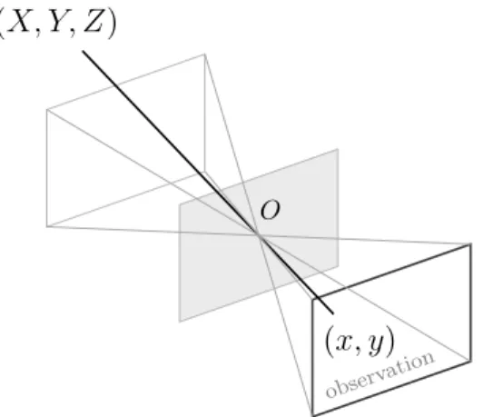
In this work we deal with both image and depth cameras that produce two-dimensional observations of a scene. Projective geometry gives many models that describe the re-lationship between real three-dimensional points in a scene and their projection onto a two-dimensional observation plane. We use the pinhole camera model, as described in Chapter 1 of Forsyth and Ponce [9]. In this camera model, a point 𝑃 in the scene – which we write as𝑊𝑃 = (𝑋, 𝑌, 𝑍)⊤for the point 𝑃 in the world coordinate frame (𝑊 ) – is linearly projected through the optical center of the camera onto point 𝑝 = (𝑥, 𝑦)⊤ in the observation plane, illustrated in Figure 2-1. Here, it is as if light were passing through a pinhole in a plane at the optical center and producing a (mirrored) image on the observation plane.
(𝑋, 𝑌, 𝑍)
(𝑥, 𝑦)
observ ation
𝑂
Figure 2-1: In the pinhole camera model, a point in the scene (𝑋, 𝑌, 𝑍) is projected onto the observation plane at (𝑥, 𝑦) through the optical center 𝑂.
We provide a brief explanation of the equations that govern the projection from
𝑊𝑃 to 𝑝, and refer readers to Forsyth and Ponce [9] for further details. Throughout
these derivations, we use boldface 𝑊𝑃 = (𝑋, 𝑌, 𝑍, 1)⊤ ∈ R4 and 𝑝 = (𝑥, 𝑦, 1)⊤ ∈ R3 to denote the homogeneous coordinate vectors corresponding to 𝑃 and 𝑝, respectively. Conceptually, this transformation can be broken down into a transformation from the scene coordinate frame (𝑊 ) into the camera coordinate frame (𝐶) (Section 2.2.1), followed by a projection onto the observation plane (Section 2.2.2).
2.2.1
Extrinsics
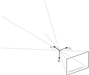
The extrinsic parameters of a camera govern the transformation from the world co-ordinate frame to the camera coco-ordinate frame. The camera coco-ordinate frame is centered at the camera’s optical center, and has 𝑥 and 𝑦 axes coplanar with the observation plane, as illustrated in Figure 2-2.
observ ation
𝑧𝑐
𝑦𝑐 𝑥𝑐
Figure 2-2: The extrinsic parameters describe the rigid body transform from the world coordinate system to the camera coordinate system, (𝑥𝑐, 𝑦𝑐, 𝑧𝑐) shown here.
The rigid body transformation from the world coordinate frame (𝑊 ) to the camera coordinate frame (𝐶) can be written as
𝐶𝑃 = ℛ𝑊𝑃 + 𝑡,
where ℛ ∈ SO(3) is a rotation matrix and 𝑡 ∈ R3 is a translation vector. In homo-geneous coordinates, we instead write
𝐶𝑃 = 𝒯 𝑊𝑃 = ⎛ ⎝ ℛ 𝑡 0⊤ 1 ⎞ ⎠𝑊𝑃 . Let 𝒯 be the extrinsic parameters of the camera.
2.2.2
Intrinsics
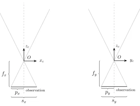
The intrinsic parameters of a camera govern how a point in the camera coordinate system is transformed to a point on the observation plane. Though there are several ways to parameterize this transform, one common approach is to use the horizontal and vertical size of the observation in pixels (𝑠𝑥, 𝑠𝑦) and the focal length (distance
from the optical center to the observation plane) in pixels (𝑓𝑥, 𝑓𝑦). Note that there
are two focal lengths, 𝑓𝑥 and 𝑓𝑦, since pixels need not be square. We also include
the principal point (𝑝𝑥, 𝑝𝑦) which represents the point on the observation plane that
is closest to the optical center (also the point where the optical axis 𝑧𝑐 intersects the
image plane). These parameters are illustrated in Figure 2-3.
𝑂 𝑧𝑐 𝑥𝑐 observation 𝑝𝑥 𝑠𝑥 𝑓𝑥 𝑂 𝑧𝑐 𝑦𝑐 observation 𝑝𝑦 𝑠𝑦 𝑓𝑦
Figure 2-3: The intrinsic parameters describe the transformation from the camera coordinate system to a point on the observation plane.
Given these parameters, we can transform a point in the camera coordinate frame to the observation space, using
𝑝 = 1 𝑍 (︁ 𝒦 0 )︁ 𝐶𝑃 ,
where 𝒦 = ⎛ ⎜ ⎜ ⎜ ⎝ 𝑓𝑥 0 𝑝𝑥 0 𝑓𝑦 𝑝𝑦 0 0 1 ⎞ ⎟ ⎟ ⎟ ⎠ is the camera calibration matrix.
Readers familiar with the pinhole camera model may notice that we omit camera skew in this derivation. In this thesis, we assume no camera skew, though it would be straightforward to incorporate.
2.3
Analysis by Synthesis
Analysis by synthesis is an approach to perception which proposes a model of the world, synthesizes expected sensory data, and compares that to real sensory data in order to evaluate the fitness of the model. In 1974, Baumgart [2] proposed vision as inverse graphics and showed that computer graphics architectures could be used as fast engines for synthesis in vision problems using this paradigm.
This approach has been used to facilitate Bayesian inference in vision [26], where probabilistic models are defined over structured representations of a scene. In particu-lar, analysis by synthesis provides a means to evaluate the likelihood of an observation given these structured representations.
2.4
Related Work
We summarize relevant work in scene understanding, categorized by inference ap-proach: sampling-based inference (Section 2.4.1) and amortized inference (Section 2.4.2).
2.4.1
Sampling-Based Inference
Here, we discuss significant works that couple a scene representation with one or more observations via a generative probabilistic model, and recover a posterior using sampling with analysis-by-synthesis.
Object-Based Representation, Single Observation
Del Pero et al. [7] modeled indoor scenes as a scene box with a collection of box-like furniture objects with relative parameters. They evaluated the likelihood of a single observation using agreement between edge features and surface normals extracted from the observations, and those implied by the model. They placed priors on object parameters and use reversible jump MCMC sampling to estimate a posterior of their scene representation and camera extrinsics. Using RJ-MCMC, they are able to handle an unknown number of objects of different types, similar to the method presented in this thesis. However, unlike in this thesis, Del Pero et al. used the same basic geometric parameterization for all object types.
Kulkarni et al. [16] proposed Picture, a probabilistic programming language for scene perception. In this method, three-dimensional scenes can be specified using a stochastic scene language, and automatic sampling-based inference using analysis by synthesis is used to recover a posterior over the scene given a single image of the scene. Kulkarni et al. give impressive examples with parameterized human faces and poses, but do not demonstrate how this method works with an unknown, variable number of objects, nor do they propose such extensions as we do in this thesis. They also showed how bottom-up, data-driven proposals can speed up the mixing time of their sampler.
Other Representations, Single Observation
Mansingkha et al. [20] presented a generative scene model, a stochastic renderer based on existing graphics software, and a likelihood model that scores rendered scenes based on a single image observation using analysis by synthesis. Their implementa-tion performed well on simple examples using single-variable random walk Metropo-lis Hastings proposals. Although they demonstrated results with three-dimensional scenes, their representation is two-dimensional and defined over the image domain. In this case, the “rendering” process used in analysis by synthesis is more akin to rasterization.
Other Representations, Multiple Observations
Cabezas, Straub and Fisher [5] presented a model that couples a mesh-based scene representation with observations from several image cameras and LiDAR, and used sampling-based inference to recover the parameterization of the mesh. They also demonstrated how to incorporate semantic labeling and a structured prior over mesh geometry and appearance as well as semantic labels to improve performance [6].
Though these works include uncertainty quantification, the low-level geometric primitives (i.e., attributed mesh polygons) that constitute the scene representation do not afford high-level reasoning about the scene in the way that the representation used in this thesis does. For example, although these works can reason over which parts of the mesh that constitutes the scene correspond to buildings, they cannot determine the number of buildings in the scene.
2.4.2
Amorized Inference
We should also mention a recent class of methods that use neural networks to amortize inference in generative scene models with object-based latent representations. Eslami et al. [8] presented a generative model for scenes with a variable number of objects, each with a type, position and orientation. Using randomly generated scenes and their renderings, they train a recurrent neural network as the encoder in an encoder-decoder architecture, with a rendering engine as the encoder-decoder. Using this network, they are able to iteratively recover the parameters of objects in novel scenes. Extensions of this work have also been proposed [15].
While these methods are impressively fast, it is unclear how they could incorporate sensor fusion without either retraining on specific sensor configurations or running inference for each sensor separately and then combining the results. The former is impractical in most realistic situations, while the latter is at best an approximation to reasoning jointly over all observations and the prior scene model.
Furthermore, it is unclear how these methods could support class-specific object parameterizations, with the fixed-length vector output of the neural networks having
Chapter 3
Model
In this chapter, we describe a generative probabilistic model that couples an object-based latent representation with multiple observations from different sensing modali-ties. The model supports a variable number of objects, each with a parameterization that depends on its type. From the generative viewpoint, the model describes how the objects in a scene give rise to multiple observations with different modalities, which allows us to reason about the likelihood that some set of objects and their parameters explain a given set of observations. This underlies the inference procedure described in Chapter 4, which allows us to recover – with uncertainty quantification – an object-based representation of a scene given such observations. Though object-object-based latent representations [7, 8, 16] and multi-modal sensor fusion [5, 6] have previously been incorporated in generative models for scene understanding, we believe that this is the first work to combine these.
We begin by outlining the components and structure of the probabilistic model, and then give further details about its parts in Sections 3.1–3.3.
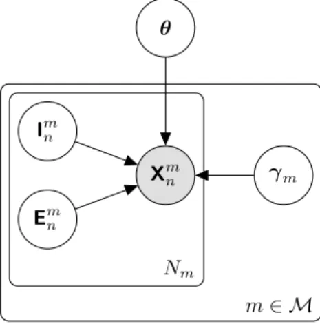
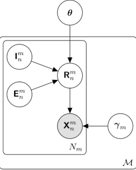
Figure 3-1 depicts the structure of the model. X𝑚𝑛 I𝑚𝑛 E𝑚𝑛 𝜃 𝛾𝑚 𝑁𝑚 𝑚 ∈ ℳ
Figure 3-1: Probabilistic model for scene, camera parameters and observations.
The latent scene model consists of 𝜃 = (c, 𝜑), which captures both the objects in a scene and their parameterization. More specifically, the scene model c is a tuple specifying the class of each object in the scene, and the scene parameterization 𝜑 is a tuple specifying the parameters of each object according to its class. Section 3.1 provides more details about this representation, as well as a structured prior model.
A set of sensor modalities ℳ are used to collect observations of the scene (outer plate in Figure 3-1). Each modality 𝑚 ∈ ℳ produces 𝑁𝑚 observations (inner plate in
Figure 3-1). For the purposes of this work, we restrict our attention to sensor modal-ities ℳ = {image, depth}, corresponding to RGB and depth cameras. Though, provided that sensor forward models can be specified, this approach can easily be extended to other modalities.
Each observation 𝑛 of modality 𝑚 is captured according to intrinsic and extrinsic camera parameters. Intrinsic parameters I = {I𝑚𝑛}𝑚,𝑛 are camera-specific parameters such as focal length or maximum depth range. Extrinsic parameters E = {E𝑚𝑛}𝑚,𝑛 describe the position and orientation of cameras relative to the scene. For simplicity, we assume that camera parameters are independent given observations, allowing us to reason over the parameters of each camera individually. This assumption is reasonable when observations come from physically distinct cameras, and could be relaxed to capture dependencies between camera parameters if this were not the case, as in [5].
Section 3.2 provides more details about camera intrinsics and extrinsics.
Observations X = {X𝑚𝑛}𝑚,𝑛 are assumed to be conditionally independent. The latent variable 𝛾𝑚parameterizes the forward model for modality 𝑚, and captures both sensor noise and any inability of the objects in a scene to fully explain the observations of this modality (e.g., due to an unmodeled scene background). Section 3.3 provides more details about 𝛾 and the forward model for each modality.
The joint probability implied by our model is
𝑝 (𝜃, 𝛾, I, E, X) = 𝑝 (𝜃) ∏︁ 𝑚∈ℳ 𝑝 (𝛾𝑚) 𝑁𝑚 ∏︁ 𝑛=1 𝑝 (I𝑚𝑛) 𝑝 (E𝑚𝑛) 𝑝 (X𝑚𝑛 | 𝜃, 𝛾𝑚, I𝑚𝑛, E𝑚𝑛) , and we explain each factor in the subsequent sections of this chapter: Section 3.1 describes 𝑝(𝜃), Section 3.2 describes 𝑝(I𝑚𝑛) and 𝑝(E𝑚𝑛), and Section 3.3 describes 𝑝(𝛾𝑚) and 𝑝 (X𝑚𝑛 | 𝜃, 𝛾𝑚, I𝑚𝑛, E𝑚𝑛).
3.1
Scene
We are interested in recovering object-based latent representations of scenes. As noted above, we represent a scene as 𝜃 = (c, 𝜑), where c is the scene model (a tuple specify-ing the class of each object in the scene), and 𝜑 is the scene parameterization (a tuple specifying the parameters of each object in the scene according to its class). Here, we give more detail on the scene model (Section 3.1.1) and the scene parameterization (Section 3.1.2), and then describe our structured scene prior (Section 3.1.3).
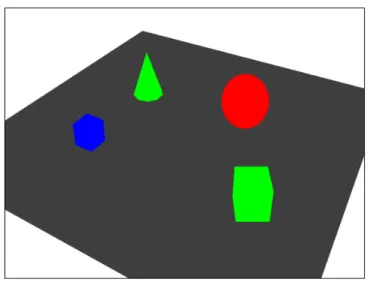
For concreteness, throughout this work we focus our attention on a simple class of scenes containing colored cubes, cones and spheres. Figure 3-2 shows an illustration of such a scene. This approach, however, is general, and could be extended to include other object classes and a more complex scene prior.
3.1.1
Model
Let 𝒞 denote the object classes (types of objects) that may be present in a scene. In our restricted case, we have 𝒞 = {cube, cone, sphere}. If there are 𝐾 objects in a
Figure 3-2: Illustration of example scene.
scene, then the scene model c = (c1, . . . , c𝐾) is a tuple of length 𝐾, where each c𝑘 ∈ 𝒞
denotes the object class of the 𝑘th object in the scene. Note that this is a symmetric representation, though the symmetry does not complicate inference.
3.1.2
Parameterization
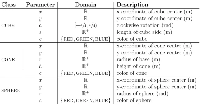
Each object class has a set of parameters that are relevant to the class. Importantly, this set of parameters may vary between classes. Table 3.1 shows the set of parameters relevant to the object classes dealt with in this work (cube, cone, sphere).
Let 𝒟𝑐 be the domain of the parameters for objects of class 𝑐. If there are 𝐾
objects in a scene, then the scene parameterization 𝜑 = (𝜑1, . . . , 𝜑𝐾) is a tuple of length 𝐾, where each 𝜑𝑘 ∈ 𝒟c𝑘 is a vector containing the parameters of the 𝑘th object
in the scene, according to its object class. Where convenient, we use the notation 𝜑𝑘,𝑙 to refer to parameter 𝑙 of object 𝑘.
Allowing object parameterization to vary across different object classes is an im-portant detail in this scene representation, for several reasons.
First, it allows us to choose parameterizations that we think are most useful for downstream tasks, and directly reason over them.
Class Parameter Domain Description
cube
𝑥 R x-coordinate of cube center (m)
𝑦 R y-coordinate of cube center (m)
𝑎 [−𝜋/4,𝜋/4) clockwise rotation (rad)
𝑠 R+ length of cube side (m)
𝑐 {red, green, blue} color of cube
cone
𝑥 R x-coordinate of cone center (m)
𝑦 R y-coordinate of cone center (m)
𝑟 R+ radius of base (m)
ℎ R+ height of cone (m)
𝑐 {red, green, blue} color of cone sphere
𝑥 R x-coordinate of sphere center (m) 𝑦 R y-coordinate of sphere center (m)
𝑟 R+ radius of sphere (rad)
𝑐 {red, green, blue} color of sphere
Table 3.1: Parameters for the cube, cone and sphere object classes.
Second, it allows us to choose parameterizations that match how we ourselves think about objects, which better positions us to encode domain knowledge in the scene prior.
Third, it allows the representation to be expressive with fewer, high-level objects. With the flexibility to choose which parameters are relevant to each object class, we can choose a set of parameters that allow us to represent many different instances of the class and explain them under the likelihood models. The benefit of this is less clear with the simple objects used in this work, though becomes more obvious as object variability increases. For example, consider including rectangular prisms in our scenes; without flexibility to choose a parameterization, we may not be able to represent the variability amongst these objects. This is obviously problematic if we care about capturing this variability for reasoning tasks. Though, even if we do not, this also cause issues if the variabilty significantly affects the likelihood, since we may not be unable to sufficiently explain observations with this object. In this instance, being able to choose an appropriate representation saves us from having to include multiple sub-types of objects (e.g., rectangular prisms with different proportions) or having to use multiple lower-level primitives to construct a higher-level object,
both of which may incur a computation cost and degrade the interpretability of the representation and its utility for downstream tasks.
Finally, it allows us to constrain the dimensionality of the representation, where appropriate. For example, spheres do not require a height parameter in the same way that cones do, and uniform spheres do not require a rotation parameter in the same way that cubes do. Excluding these parameters reduces the dimensionality of the parameter space that we must perform inference over, which reduces computational complexity. The benefit of this grows with the number of objects, as the union of parameters relevant to all objects becomes large.
3.1.3
Prior
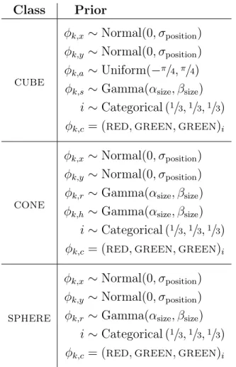
The model allows us to encode prior knowledge about the scene structure and param-eters with a prior 𝑝(𝜃) = 𝑝(c, 𝜑). For this work, we choose a relatively uninformative prior about the number of objects in a scene and the parameters of these objects, reweighted by the hard constraint that objects cannot overlap each other.
Let 𝑁𝑐 be the number of objects of class 𝑐. Then we choose
𝑝(𝜃) = 𝑝(c, 𝜑) ∝ 𝜓(c, 𝜑) (︃ ∏︁ 𝑐 Poisson(𝑁𝑐; 𝜆𝑐) )︃ (︃ 𝐾 ∏︁ 𝑘=1 𝑝c𝑘(𝜑𝑘) )︃ , where 𝜓(c, 𝜑) = ⎧ ⎪ ⎨ ⎪ ⎩
0 if the footprints of any two shapes overlap 1 otherwise
enforces the constraint that objects cannot overlap, and 𝑝𝑐(𝜑𝑘) are class-specific
parameter priors, specified in Table 3.2. For each of these parameter priors, we set 𝜎position = 2.5, 𝛼size= 2 and 𝛽size=1/3.
Though this prior is relatively straightforward, in the general case there is no restriction on the scene prior except that we must be able to evaluate it to within some constant factor. This provides a powerful way to encode domain knowledge.
Class Prior
cube
𝜑𝑘,𝑥 ∼ Normal(0, 𝜎position)
𝜑𝑘,𝑦 ∼ Normal(0, 𝜎position)
𝜑𝑘,𝑎 ∼ Uniform(−𝜋/4,𝜋/4)
𝜑𝑘,𝑠 ∼ Gamma(𝛼size, 𝛽size)
𝑖 ∼ Categorical (1/3,1/3,1/3)
𝜑𝑘,𝑐 = (red, green, green)𝑖
cone
𝜑𝑘,𝑥 ∼ Normal(0, 𝜎position)
𝜑𝑘,𝑦 ∼ Normal(0, 𝜎position)
𝜑𝑘,𝑟 ∼ Gamma(𝛼size, 𝛽size)
𝜑𝑘,ℎ ∼ Gamma(𝛼size, 𝛽size)
𝑖 ∼ Categorical (1/3,1/3,1/3)
𝜑𝑘,𝑐 = (red, green, green)𝑖
sphere
𝜑𝑘,𝑥 ∼ Normal(0, 𝜎position)
𝜑𝑘,𝑦 ∼ Normal(0, 𝜎position)
𝜑𝑘,𝑟 ∼ Gamma(𝛼size, 𝛽size)
𝑖 ∼ Categorical (1/3,1/3,1/3)
𝜑𝑘,𝑐 = (red, green, green)𝑖
Table 3.2: Priors for cube, cone and sphere parameters.
3.2
Sensors
The model supports both image and depth cameras. For both the image and depth modalities, we assume ideal pinhole cameras (Section 2.2). For each observation X𝑚𝑛, we associate corresponding extrinsic (E𝑚𝑛) and intrinsic (I𝑚𝑛) sensor parameters.
3.2.1
Extrinsics
For both image and depth cameras, the extrinsic parameters specify the optical center and direction of the optical axis. We represent this as a rigid transformation from the scene coordinate system to the camera coordinate system shown as (𝑥𝑐, 𝑦𝑐, 𝑧𝑐) in
observation
𝑧𝑐
𝑦𝑐 𝑥𝑐
Figure 3-3: Sensor extrinsics.
We use the special Euclidean group of rigid transformations in R3, with
E𝑚𝑛 ∈ SE(3) ∀ 𝑚 ∈ {image, depth}, ∀ 𝑛 = 1, . . . , 𝑁𝑚.
3.2.2
Intrinsics
Cameras are parameterized by the width and height of the images they produce in pixels, 𝑠𝑥 and 𝑠𝑦, respectively; the horizontal and vertical focal length in pixels, 𝑓𝑥
and 𝑓𝑦, respectively; and the principle point of the image in pixels, (𝑝𝑥, 𝑝𝑦). These
values are shown graphically in Figure 3-4. For image cameras, we have
Iimage
𝑛 = (𝑠𝑥, 𝑠𝑦, 𝑓𝑥, 𝑓𝑦, 𝑝𝑥, 𝑝𝑦) ∀ 𝑛 = 1, . . . , 𝑁image.
For depth cameras, we include an additional intrinsic parameter 𝑑max corresponding
to the maximum observable depth, Idepth
𝑂 𝑧𝑐 𝑥𝑐 observation 𝑝𝑥 𝑠𝑥 𝑓𝑥 𝑂 𝑧𝑐 𝑦𝑐 observation 𝑝𝑦 𝑠𝑦 𝑓𝑦
Figure 3-4: Sensor intrinsics.
3.2.3
Prior
The model allows for a prior over intrinsic and extrinsic camera parameters. Fur-thermore, these parameters could theoretically be recovered given observations, with a slight modification to the inference procedure describe in Chapter 4. However, for simplicity, in this thesis we treat camera parameters as known.
3.3
Observations
Both image and depth observations occur as two-dimensional pixel grids. Image pixels have three channels (RGB intensities ranging from 0 to 1). Depth pixels have a single channel that represents the distance from the optical center to the observed object, clipped at the maximum observable distance, 𝑑max. We use 𝑢 (horizontal pixel
position), 𝑣 (vertical pixel position) and 𝑤 (channel) to denote observations indices, such as Ximage
𝑛 (𝑢, 𝑣, 𝑤) and Xdepth𝑛 (𝑢, 𝑣).
to evaluate the likelihood 𝑝 (X | 𝜃, 𝛾, I, E) = ∏︁ 𝑚∈ℳ 𝑁𝑚 ∏︁ 𝑛=1 𝑝 (X𝑚𝑛 | 𝜃, 𝛾𝑚, I𝑚𝑛, E𝑚𝑛) .
However, it is difficult to derive a closed-form expression for this likelihood, due to the nonparametetric, object-based latent representation we use for scenes. In particular, the pixels of an observation may be associated with any one (or none) of the objects in a scene, and which object each pixel is attributable to is a complex function of all of the objects’ classes and parameters, as well as the intrinsic and extrinsic camera parameters associated with the observation. For this reason, we employ analysis by synthesis (Section 2.3) to approximate the likelihood, by synthesizing pseudo-observations of the scene under the given scene representation and camera parameters, and comparing these to the true observations.
For each observation X𝑚𝑛, we introduce the intermediate variables R𝑚𝑛 for the pseudo-observations, with dimensionality equal to the corresponding observation. We let R𝑚𝑛 = 𝑟𝑚(𝜃, I𝑚𝑛, E
𝑚
𝑛), where 𝑟𝑚is a modality-specific, deterministic rendering
func-tion, described in Section 3.3.1. We assume that each observation is independent given its pseudo-observation and noise parameters, and describe X𝑚𝑛 ∼ 𝑝 (X𝑚𝑛 | R𝑚𝑛, 𝛾𝑚) for the image and depth modalities in Sections 3.3.2 and 3.3.3, respectively. This decom-position of the likelihood is visualized in Figure 3-5.
Now as long as we can evaluate X𝑚𝑛 ∼ 𝑝 (X𝑚 𝑛 | R
𝑚
𝑛, 𝛾𝑚), we can evaluate the
likelihood as 𝑝 (X𝑚𝑛 | 𝜃, 𝛾𝑚, I𝑚𝑛, E𝑚𝑛) =∑︁ R𝑚𝑛 𝑝 (X𝑚𝑛 | 𝛾𝑚, R𝑚𝑛) 𝑝 (R𝑚𝑛 | 𝜃, I𝑚 𝑛, E 𝑚 𝑛) = 𝑝 (X𝑚𝑛 | 𝛾𝑚, R𝑚𝑛 = 𝑟𝑚(𝜃, I𝑚𝑛, E 𝑚 𝑛)) , since R𝑚𝑛 = 𝑟𝑚(𝜃, I𝑚𝑛, E 𝑚 𝑛) is deterministic.
X𝑚𝑛 R𝑚𝑛 I𝑚𝑛 E𝑚𝑛 𝜃 𝛾𝑚 𝑁𝑚 ℳ
Figure 3-5: We introduce pseudo-observations R𝑚𝑛 = 𝑟𝑚(𝜃, I𝑚𝑛, E 𝑚
𝑛) which are
de-terministically rendered using the scene representation and camera parameters, and assume X𝑚𝑛 ∼ 𝑝 (X𝑚
𝑛 | R 𝑚
𝑛, 𝛾𝑚) are conditionally independent.
3.3.1
Rendering Function
Modern computer graphics pipelines can be used to produce pseudo-observations from the object-based latent representation, as well as sensor intrinsics and extrinsics. Objects in our latent space correspond closely to objects in a computer graphics scene graph. Given a canonical mesh for each object class as well as how object parameters perturb this mesh, it is straightforward to render pseudo-observations.
As a part of this work, we implement rendering functions that map object param-eters, as well as intrinsics and extrinsics to pseudo-observations for both the image and depth modalities. We use the Panda3D graphics engine [12] as the basis of our implementation, and define basic mesh models for the unit cube, cone and sphere, as well as how object parameters perturb this mesh. As a part of this implementation, we also define custom shaders to quickly render depth pseudo-observations.
3.3.2
Image Likelihood
For the image modality, we assume observations follow Ximage 𝑛 (𝑢, 𝑣, 𝑤) = Rimage𝑛 (𝑢, 𝑣, 𝑤) + 𝜖image𝑛 (𝑢, 𝑣, 𝑤) ∀ 𝑛, 𝑢, 𝑣, 𝑤, where 𝜖image 𝑛 (𝑢, 𝑣, 𝑤) i.i.d. ∼ Normal (0, 𝛾image) and we place a Gamma prior on 𝛾image.
We also take advantage of computer graphics pipelines to evaluate 𝑝 (Ximage
𝑛 | Rimage𝑛 , 𝛾image) = Normal (X image
𝑛 − Rimage𝑛 ; 0, 𝛾image) .
Here we load Ximage
𝑛 into graphics memory, render Rimage𝑛 to graphics memory, and
then compute the normal density on the GPU.
3.3.3
Depth Likelihood
Similarly, for the depth modality, we assume observations follow Xdepth 𝑛 (𝑢, 𝑣) = Rdepth𝑛 (𝑢, 𝑣) + 𝜖depth𝑛 (𝑢, 𝑣) ∀ 𝑛, 𝑢, 𝑣 where 𝜖depth 𝑛 (𝑢, 𝑣) i.i.d. ∼ Normal (0, 𝛾depth) and we place a Gamma prior on 𝛾depth.
3.4
Discussion
Here we described a probabilistic model that couples an object-based latent scene representation with multiple observations with different modalities. Though we made this model concrete by considering a specific class of scenes with simple shape objects,
the approach described here is general, and applies to a much broader range of scenes with more complex objects.
Chapter 4
Inference
In this chapter we describe a sampling-based inference procedure for the probabilistic model defined in Chapter 3. This procedure draws samples from the posterior distri-bution 𝑝 (𝜃 | 𝑋, 𝐼, 𝐸) over the scene representation 𝜃, given a set of observations X and their associated camera parameters I and E. Recall that we represent scenes as 𝜃 = (c, 𝜑) where c is the scene model c (the class of each object in the scene), and 𝜑 is the scene parameterization (the class-specific parameterization of each object). Thus, we really draw samples from 𝑝 (c, 𝜑 | 𝑋, 𝐼, 𝐸). Given samples from the posterior, we can obtain a point estimate of the scene by taking the maximum a posteriori sample, or compute statistics over these samples to provide uncertainty quantification.
Our contribution with this method is twofold. First, we show how to infer an object-based representation of a scene using multiple observations of different modal-ities. While previous methods [16, 8, 7] have demonstrated the ability to recover an object-based representation of a scene, we believe this is the first method to in-corporate multiple sensors and modalities. This is particularly important in scene understanding problems, as information is often distributed across multiple obser-vations, particularly for large scenes. Second, we introduce object change proposals between objects with different parameterizations in our sampling procedure in order to speed up sampler convergence.
We begin by outlining the full inference procedure at a high level, followed by the details of each inference step.
Algorithm 1 shows the top-level inference produce. We use Gibbs sampling to draw samples from the joint conditional 𝑝 (c, 𝜑, 𝛾 | 𝑋, 𝐼, 𝐸) – by alternating sampling the objects in the scene and their parameters (c, 𝜑) ∼ 𝑝 (c, 𝜑 | 𝛾, X, I, E), and noise parameters 𝛾 ∼ 𝑝 (𝛾 | c, 𝜑, X, I, E) – and marginalize out 𝛾 (by ignoring samples of 𝛾). We initialize the scene to be empty (no objects), and draw the initial 𝛾 from its prior.
Algorithm 1: Inference
Input: observations X, camera parameters I, E, number of samples 𝑇 Result: samples 𝜃(1), . . . , 𝜃(𝑇 ) 1 c(0), 𝜑(0) ← 𝑒𝑚𝑝𝑡𝑦 2 𝛾(0) ∼ 𝑝 (𝛾) 3 for 𝑛 = 1, . . . , 𝑇 do 4 c(𝑡), 𝜑(𝑡) ← SampleScene (︁ c(𝑡−1), 𝜑(𝑡−1), 𝛾(𝑡−1), X, I, E)︁ 5 𝛾(𝑡) ← SampleNoiseParameters (︁ c(𝑡), 𝜑(𝑡), 𝛾(𝑡−1), X, I, E)︁ 6 𝜃(𝑡) ← (︁ c(𝑡), 𝜑(𝑡))︁ 7 end 8 return 𝜃(1), . . . , 𝜃(𝑇 )
The subroutines SampleScene (line 4) and SampleNoiseParameters (line 5) handle sampling from 𝑝 (c, 𝜑 | 𝛾, X, I, E) and 𝑝 (𝛾 | c, 𝜑, X, I, E), and are covered in Sections 4.1 and 4.2, respectively.
4.1
Sampling Scene
Standard MCMC sampling is not sufficient for drawing samples from 𝑝 (c, 𝜑 | 𝛾, X, I, E), since both c and 𝜑 have variable dimensionality. Thus, we use reversible-jump Markov chain Monte Carlo (RJ-MCMC) to draw samples from this conditional. In particular, we make use of four move types:
1. updating object parameters; 2. birth of a new object;
3. death of an existing object; 4. changing an object’s class.
Moves (2) and (3) necessarily involve a change in the dimensionality of (c, 𝜑). Move (4) may also involve a change in the dimensionality of 𝜑, depending on the class of the object being changed. Algorithm 2 describes the high-level procedure for sampling from the full conditional over the scene representation. Note that we introduce the paramter 𝑝model, which is the probability of performing a model jump by making one
of moves (2)–(4). In our work we set 𝑝model=1/20.
Algorithm 2: SampleScene
Input: scene model c, object parameters 𝜑, noise parameters 𝛾, observations X, camera parameters I, E
Parameters: probability of proposing model jump 𝑝model
Result: new sample of scene model cnew and object parameters 𝜑new
1 c𝑛𝑒𝑤 ← c 2 𝜑𝑛𝑒𝑤 ← 𝜑 3 𝐾 ← Length(c) 4 for 𝑘 ∈ {1, . . . , 𝐾} do 5 𝜑𝑛𝑒𝑤𝑘 ← SampleObjectParameters (𝑘, c, 𝜑𝑛𝑒𝑤, 𝛾, X, I, E) 6 end 7 𝑢 ∼ Uniform(0, 1) 8 if 𝑢 < 𝑝model then 9 c𝑛𝑒𝑤, 𝜑𝑛𝑒𝑤 ← SampleSceneModel (c𝑛𝑒𝑤, 𝜑𝑛𝑒𝑤, 𝛾, X, I, E) 10 end 11 return c𝑛𝑒𝑤, 𝜑𝑛𝑒𝑤
We first perform move (1), and use Gibbs sampling to sample new parameters for each object 𝑘 = 1, . . . , 𝐾 in the scene (lines 1–6). Here, we sample from the full conditional of each object’s parameters separately. In reality, the parameters of different objects may be tightly coupled, particularly when they are close to one another. For this reason, one could consider an alternative implementation where object parameters were occasionally sampled from the joint over all objects. However, we found this approach of sampling objects individually to be sufficient for our work. The subroutine SampleObjectParameters (line 5) handles sampling from the full conditional 𝑝(︀𝜑𝑘 | c, 𝜑−𝑘, 𝛾, X, I, E)︀, and is described in Section 4.1.1.
With probability 𝑝model, we also perform one of moves (2)–(4) and sample a model
jump. This may result in adding an object to the scene, removing an object from the scene, or changing an object’s class, all of which may the dimensionality of the latent scene representation. Here, we jointly sample the scene model c and any new object parameters that a model jump introduces, conditioned on all other variables. The subroutine SampleSceneModel (line 9) handles this, and is described in Sec-tion 4.1.2.
4.1.1
Sampling Object Parameters
When sampling an object’s parameters, we sample from the joint of all of parameters for this object, conditioned on all other variables. That is, when sampling object 𝑘’s parameters, we sample from 𝑝(︀𝜑𝑘| c, 𝜑−𝑘, 𝛾, X, I, E)︀. We use the Metropolis-Hastings algorithm [14] to sample from this distribution. Our procedure is shown in Algorithm 3, with the proposals and acceptance probability (line 9) derived subse-quently.
Algorithm 3: SampleObjectParameters
Input: index of object to sample 𝑘, scene model c, object parameters 𝜑, noise parameters 𝛾, observations X, camera parameters I, E Result: new sample of object 𝑘’s parameters 𝜑new𝑘
1 if c𝑘= cube then
2 𝜑′𝑘 ← ProposeCube(𝜑𝑘) 3 else if c𝑘 = cone then 4 𝜑′𝑘 ∼ ProposeCone(𝜑𝑘) 5 else 6 𝜑′𝑘 ← ProposeSphere(𝜑𝑘) 7 end 8 𝑢 ∼ Uniform(0, 1) 9 if 𝑢 < 𝐴 (𝜑′𝑘, 𝜑𝑘) then 10 return 𝜑′𝑘 11 else 12 return 𝜑𝑘 13 end
Proposals
We use symmetric proposal distributions for object parameter sampling. All nu-merical parameters proposals are drawn from Gaussian distributions centered at the current parameter’s value. For simplicity, these Gaussian proposal distributions all share the same variance 𝜎2proposal, though this need not be the case. The proposal for the discrete color parameter is selected uniformly from all colors. Algorithms 4, 5 and 6 show the procedure for generating parameter proposals for cubes, cone and spheres, respectively. We do not explicitly derive proposal densities, since they are symmetric and can be ignored from the calculation of the Hastings ratio.
Algorithm 4: ProposeCube Input: current cube parameters 𝜑𝑘 Result: proposed cube parameters 𝜑′𝑘
1 for 𝑙 ∈ {x-position, y-position, rotation, side-length} do 2 𝜑′𝑘,𝑙 ∼ Normal(︀𝜑𝑘,𝑙, 𝜎proposal2 )︀
3 end
4 𝑖 ∼ Categorial (3, (1/3,1/3,1/3)) 5 𝜑′𝑘,color ← (red, green, blue)𝑖 6 return 𝜑′𝑘
Algorithm 5: ProposeCone Input: current cone parameters 𝜑𝑘 Result: proposed cone parameters 𝜑′𝑘
1 for 𝑙 ∈ {x-position, y-position, radius, height} do 2 𝜑′𝑘,𝑙 ∼ Normal(︀𝜑𝑘,𝑙, 𝜎proposal2 )︀
3 end
4 𝑖 ∼ Categorial (3, (1/3,1/3,1/3)) 5 𝜑′𝑘,color ← (red, green, blue)𝑖 6 return 𝜑′𝑘
Algorithm 6: ProposeSphere Input: current sphere parameters 𝜑𝑘 Result: proposed sphere parameters 𝜑′𝑘
1 for 𝑙 ∈ {x-position, y-position, radius} do 2 𝜑′𝑘,𝑙 ∼ Normal(︀𝜑𝑘,𝑙, 𝜎proposal2 )︀
3 end
4 𝑖 ∼ Categorial (3, (1/3,1/3,1/3)) 5 𝜑′𝑘,color ← (red, green, blue)𝑖 6 return 𝜑′𝑘
Acceptance Probability
For the acceptance probability we have
𝐴 (𝜑′𝑘, 𝜑𝑘) = min (︃ 1,𝑝(︀𝜑 ′ 𝑘| c, 𝜑−𝑘, 𝛾, X, I, E)︀ 𝑞(𝜑𝑘 | 𝜑 ′ 𝑘) 𝑝(︀𝜑𝑘| c, 𝜑−𝑘, 𝛾, X, I, E)︀ 𝑞(𝜑 ′ 𝑘 | 𝜑𝑘) )︃ ,
where 𝑞 is the proposal distribution for the relevant object class. Since we chose symmetric proposal distributions for all objects, we have 𝑞(𝜑𝑘 | 𝜑′𝑘) = 𝑞(𝜑′𝑘| 𝜑𝑘) and
𝑝(︀𝜑′𝑘 | c, 𝜑−𝑘, 𝛾, X, I, E)︀ 𝑞(𝜑𝑘| 𝜑′𝑘) 𝑝(︀𝜑𝑘 | c, 𝜑−𝑘, 𝛾, X, I, E)︀ 𝑞(𝜑 ′ 𝑘| 𝜑𝑘) = 𝑝(︀𝜑 ′ 𝑘 | c, 𝜑−𝑘, 𝛾, X, I, E )︀ 𝑝(︀𝜑𝑘 | c, 𝜑−𝑘, 𝛾, X, I, E )︀ .
Let 𝜑′ = (︀𝜑:𝑘−1, 𝜑′𝑘, 𝜑𝑘+1:)︀ be the parameters of all objects after the proposal, in-cluding the new parameters proposed for object 𝑘. Then we have
𝑝(︀𝜑′𝑘| c, 𝜑−𝑘, 𝛾, X, I, E)︀ 𝑝(︀𝜑𝑘| c, 𝜑−𝑘, 𝛾, X, I, E )︀ = 𝑝 (c, 𝜑′, 𝛾, X, I, E) 𝑝 (c, 𝜑, 𝛾, X, I, E) = 𝑝 (c) 𝑝 (𝜑 ′ | c) 𝑝 (𝛾) 𝑝 (X | c, 𝜑′ , 𝛾, I, E) 𝑝 (c) 𝑝 (𝜑 | c) 𝑝 (𝛾) 𝑝 (X | c, 𝜑, 𝛾, I, E) = 𝑝 (𝜑 ′ | c) 𝑝 (X | c, 𝜑′, 𝛾, I, E) 𝑝 (𝜑 | c) 𝑝 (X | c, 𝜑, 𝛾, I, E)
Finally, we get the acceptance probability 𝐴 (𝜑′𝑘, 𝜑𝑘) = min (︂ 1,𝑝 (𝜑 ′ | c) 𝑝 (X | c, 𝜑′ , 𝛾, I, E) 𝑝 (𝜑 | c) 𝑝 (X | c, 𝜑, 𝛾, I, E) )︂ .
This amounts to computing the prior over the scene parameterization and the likeli-hood for each observation, both before and after the proposal. Note that if a proposal results in one or more overlapping objects, then 𝑝 (𝜑′ | c) = 0, and we would always reject this proposal. In our implementation, the prior and likelihood from before the proposal have been previously computed and stored for efficiency.
4.1.2
Sampling Scene Model
Sampling object parameters alone is not sufficient to ensure the ergodicity of the sampler. Since it is not known which objects comprise the scene, we must also include sampling proposals which change the number and classes of objects. We do this with model jump moves, which change the dimensionality of the latent representation.
In this thesis, we include three such moves: birth moves, death moves and change moves. When sampling the scene model, we perform any one of these moves with equal probability. Since remove and change moves only make sense when there is at least one object in the scene, they are skipped when there are no objects in the current sample.
Algorithm 7 describes the high-level procedure for sampling the scene model, and the subroutines for birth, death and change moves are detailed in the remainder of this section.
Algorithm 7: SampleSceneModel
Input: current scene model c, current object parameters 𝜑, current noise parameters 𝛾, observations X, camera parameters I, E
Result: new sample of scene model cnew and parameters 𝜑new 1 𝐾 ← length(c) 2 𝑢 ∼ Uniform(0, 1) 3 if 𝑢 <1/3 then 4 return SampleBirth(c, 𝜑, 𝛾, X, I, E) 5 else if 𝑢 <2/3 then 6 if 𝐾 > 0 then 7 return SampleDeath(c, 𝜑, 𝛾, X, I, E) 8 end 9 else 10 if 𝐾 > 0 then 11 return SampleChange(c, 𝜑, 𝛾, X, I, E) 12 end 13 end 14 return c, 𝜑 Birth Moves
When sampling a birth move in a scene with 𝐾 objects, we propose the addition of object 𝐾 + 1 with class 𝑐 selected uniformly at random, and propose the parameters of the new object by sampling them from the relevant object class parameter prior 𝜑′𝐾+1 ∼ 𝑝𝑐(·) (see Section 3.1.3 for details on these parameter priors). Algorithm 8
details this process, with the acceptance probability (line 16) derived subsequently. This type of move changes the dimensionality of both the scene model c (since a new object is introduced) and the scene parameterization 𝜑 (since parameters for this object are introduced). Given this, the acceptance probability is more complex than in the case of sampling object parameters, and must account for the change in dimensionality. Background on the acceptance probability for proposals which change dimensionality can be found in Section 2.1.3.
Algorithm 8: SampleBirth
Input: current scene model c, current object parameters 𝜑, current noise parameters 𝛾, observations X, camera parameters I, E
Result: new sample of scene model cnew and parameters 𝜑new 1 𝐾 ← Length(c) 2 c′ ← c 3 𝜑′ ← 𝜑 4 𝑢 ∼ Uniform(0, 1) 5 if 𝑢 <1/3 then 6 c′𝐾+1 ← cube 7 𝜑′𝐾+1 ∼ 𝑝cube(·) 8 else if 𝑢 <2/3 then 9 c′𝐾+1 ← cone 10 𝜑′𝐾+1 ∼ 𝑝cone(·) 11 else 12 c′𝐾+1 ← sphere 13 𝜑′𝐾+1 ∼ 𝑝sphere(·) 14 end 15 𝑤 ∼ Uniform(0, 1) 16 if 𝑤 < 𝐴 ((c′, 𝜑′), (c, 𝜑)) then 17 return c′, 𝜑′ 18 else 19 return c, 𝜑 20 end
Let 𝑐 be the selected object class to add, and 𝜑′𝐾+1 be the new parameters intro-duced by this model jump. The acceptance probability is then
𝐴 ((c′, 𝜑′), (c, 𝜑)) = min (︃ 1,𝑝 (c ′, 𝜑′ | 𝛾, X, I, E) 𝑝 (c, 𝜑 | 𝛾, X, I, E) · 𝑟′(c′, 𝜑′) 𝑟 (c, 𝜑) 𝑝𝑐(︀𝜑′𝐾+1 )︀ · ⃒ ⃒ ⃒ ⃒ ⃒ 𝜕𝜑′ 𝜕(︀𝜑, 𝜑′ 𝐾+1 )︀ ⃒ ⃒ ⃒ ⃒ ⃒ )︃ where 𝑟(c, 𝜑) = 𝑝model ⏟ ⏞ model jump · 1/3 ⏟ ⏞ birth move · 1/3 ⏟ ⏞ object class
is the probability of making a birth move and introducing an object of class 𝑐, and 𝑟′(c′, 𝜑′) = 𝑝model ⏟ ⏞ model jump · 1/3 ⏟ ⏞ death move · 1/𝐾 + 1 ⏟ ⏞ object to remove
is the probability of making the inverse death move (detailed in the next section) and removing the object starting from state (c′, 𝜑′). Now since we are simply appending parameters to the scene parameterization and 𝜑′ = (𝜑, 𝜑′𝐾+1), we have that the Jacobian,
𝜕𝜑′ 𝜕(︀𝜑, 𝜑′𝐾+1)︀ ,
is simply the identity matrix, and therefore the Jacobian determinant is ⃒ ⃒ ⃒ ⃒ ⃒ 𝜕𝜑′ 𝜕(︀𝜑, 𝜑′𝐾+1)︀ ⃒ ⃒ ⃒ ⃒ ⃒ = 1
We can then simplify 𝑝 (c′, 𝜑′ | 𝛾, X, I, E) 𝑝 (c, 𝜑 | 𝛾, X, I, E) · 𝑟′(c′, 𝜑′) 𝑟 (c, 𝜑) 𝑝𝑐(𝜑′𝑘) · ⃒ ⃒ ⃒ ⃒ 𝜕𝜑′ 𝜕 (𝜑, 𝜑′𝑘) ⃒ ⃒ ⃒ ⃒ = 𝑝 (c ′, 𝜑′ | 𝛾, X, I, E) 𝑝 (c, 𝜑 | 𝛾, X, I, E) · 3 (𝐾 + 1)𝑝𝑐(𝜑′𝑘) = 𝑝 (c ′) 𝑝 (𝜑′ | c′) 𝑝 (X | c′, 𝜑′ , 𝛾, I, E) 𝑝 (c) 𝑝 (𝜑 | c) 𝑝 (X | c, 𝜑, 𝛾, I, E) · 3 (𝐾 + 1)𝑝𝑐(𝜑′𝑘) . There are two distinct factors in this term. On the left, we have
𝑝 (c′) 𝑝 (𝜑′ | c′) 𝑝 (X | c′, 𝜑′
, 𝛾, I, E) 𝑝 (c) 𝑝 (𝜑 | c) 𝑝 (X | c, 𝜑, 𝛾, I, E)
which is the ratio of the posterior probability of the scene and observations under the proposal, to the posterior probability under the original sample. Intuitively, this increases the probability of accepting proposals which are more likely under the observations and scene prior. On the right we have
3
(𝐾 + 1)𝑝𝑐(𝜑′𝑘)
,
which is the ratio of the probability of making the inverse proposal (a death move) from the proposed state back to the current state, to the probability of making this birth move proposal from the current state. Together, these ensure that we satisfy detailed balance.
Death Moves
When sampling a death move in a scene with 𝐾 > 0 objects, we select one of the objects 𝑘 uniformly at random and propose removing it from the scene (removing c𝑘
and 𝜑𝑘). Algorithm 9 details this process. Algorithm 9: SampleDeath
Input: current scene model c, current object parameters 𝜑, current noise parameters 𝛾, observations X, camera parameters I, E
Result: new sample of scene model cnew and parameters 𝜑new 1 𝐾 ← Length(c) 2 𝑘 ∼ Categorical (𝐾, (1/𝐾, . . . ,1/𝐾)) 3 c′ ← (c:𝑘−1, c𝑘+1:) 4 𝜑′ ←(︀𝜑:𝑘−1, 𝜑𝑘+1:)︀ 5 𝑢 ∼ Uniform(0, 1) 6 if 𝑢 < 𝐴 ((c′, 𝜑′), (c, 𝜑)) then 7 return c′, 𝜑′ 8 else 9 return c, 𝜑 10 end
Let 𝑐 be the class of the object selected for removal, and 𝜑𝑘 be the parameters removed by this model jump. The acceptance probability (line 6) is then
𝐴 ((c′, 𝜑′), (c, 𝜑)) = min (︂ 1,𝑝 (c ′, 𝜑′ | 𝛾, X, I, E) 𝑝 (c, 𝜑 | 𝛾, X, I, E) · 𝑟′(c′, 𝜑′) 𝑝𝑐(𝜑𝑘) 𝑟 (c, 𝜑) · ⃒ ⃒ ⃒ ⃒ 𝜕 (𝜑′, 𝜑𝑘) 𝜕𝜑 ⃒ ⃒ ⃒ ⃒ )︂ where 𝑟(c, 𝜑) = 𝑝model ⏟ ⏞ model jump · 1/3 ⏟ ⏞ death move · 1/𝐾 ⏟ ⏞ object to remove
is the probability of making this death move, 𝑟′(c′, 𝜑′) = 𝑝model ⏟ ⏞ model jump · 1/3 ⏟ ⏞ birth move · 1/3 ⏟ ⏞ object class
is the probability of making the inverse birth move to introduce an object with the same class as the one removed, and 𝑝𝑐(𝜑𝑘) is the probability of choosing the same
parameters as the object removed during this birth move. Since 𝜑′ is simply 𝜑 with parameters 𝜑𝑘 removed, we have that the Jacobian
𝜕 (𝜑′, 𝜑𝑘) 𝜕𝜑
is some permutation of the identity matrix (where the exact permutation depends on the object chosen to remove, 𝑘) and therefore
⃒ ⃒ ⃒ ⃒ 𝜕 (𝜑′, 𝜑𝑘) 𝜕𝜑 ⃒ ⃒ ⃒ ⃒ = 1. Given this, we can simplify
𝑝 (c′, 𝜑′ | 𝛾, X, I, E) 𝑝 (c, 𝜑 | 𝛾, X, I, E) · 𝑟′(c′, 𝜑′) 𝑝𝑐(𝜑𝑘) 𝑟 (c, 𝜑) · ⃒ ⃒ ⃒ ⃒ 𝜕 (𝜑′, 𝜑𝑘) 𝜕𝜑 ⃒ ⃒ ⃒ ⃒ = 𝑝 (c ′, 𝜑′ | 𝛾, X, I, E) 𝑝 (c, 𝜑 | 𝛾, X, I, E) · 𝐾 · 𝑝𝑐(𝜑𝑘) 3 = 𝑝 (c ′) 𝑝 (𝜑′ | c′) 𝑝 (X | c′, 𝜑′ , 𝛾, I, E) 𝑝 (c) 𝑝 (𝜑 | c) 𝑝 (X | c, 𝜑, 𝛾, I, E) · 𝐾 · 𝑝𝑐(𝜑𝑘) 3 .
Similar to the acceptance probability for birth moves, we have two distinct factors. The left factor deals with the posterior probability before and after the proposal, and the right factor deals with the probability of making the inverse birth move versus this death move. Together, these ensure that we satisfy detailed balance.
Change Moves
Birth and death moves are sufficient to ensure the ergodicity of our sampler. However, if in the course of sampling, some object provides a reasonable explanation for parts of observations that are in fact due to an object of some other class (for example, if a sphere is positioned where a cube should be), then sampling may take a long time to converge to the correct object class. For this reason, we include change moves as a third type of model jump. When sampling a change move in a scene with 𝐾 > 0 objects, we select one of the objects 𝑘 uniformly at random and propose changing its class to one of the other object classes, also uniformly at random.
Algorithm 10: SampleChange
Input: current scene model c, current object parameters 𝜑, current noise parameters 𝛾, observations X, camera parameters I, E
Result: new sample of scene model cnew and parameters 𝜑new 1 𝐾 ← Length(c) 2 𝑘 ∼ Categorical (𝐾, (1/𝐾, . . . ,1/𝐾)) 3 c′ ← c 4 𝜑′ ← 𝜑 5 𝑢 ∼ Uniform(0, 1) 6 if c𝑘= cube then 7 if 𝑢 <1/2 then 8 c′𝑘 ← cone 9 𝜑′𝑘 ← ProposeConeFromCube(𝜑𝑘) 10 else 11 c′𝑘 ← sphere 12 𝜑′𝑘 ← ProposeSphereFromCube(𝜑𝑘) 13 end
14 else if c𝑘 = cone then 15 if 𝑢 <1/2 then 16 c′𝑘 ← cube 17 𝜑′𝑘 ← ProposeCubeFromCone(𝜑𝑘) 18 else 19 c′𝑘 ← sphere 20 𝜑′𝑘 ← ProposeSphereFromCone(𝜑𝑘) 21 end 22 else 23 if 𝑢 <1/2 then 24 c′𝑘 ← cube 25 𝜑′𝑘 ← ProposeCubeFromSphere(𝜑𝑘) 26 else 27 c′𝑘 ← cone 28 𝜑′𝑘 ← ProposeConeFromSphere(𝜑𝑘) 29 end 30 𝑤 ∼ Uniform(0, 1) 31 if 𝑤 < 𝐴 ((c′, 𝜑′), (c, 𝜑)) then 32 return c′, 𝜑′ 33 else 34 return c, 𝜑 35 end
Algorithm 10 details the process for sampling a change move. When proposing parameters for the new object, we choose to hold similar parameters constant and sample other parameters from their priors. In particular, we hold the x- and y-position constant for change moves between any two object classes. The rationale behind these proposals is to increase the acceptance probability – if we have an object of one class that explains the observations reasonably well (e.g., a sample with a red sphere positioned roughly where a red cube should be), then it is more likely that proposing an object of a different class will be accepted if we constrain parameters that are similar across object classes to the same neighborhood. We could have designed proposals that captured more complicated relationships between other parameters of different object classes, though we found these proposals to be sufficient.
In each change proposal, some object parameters are held constant, some are introduced, and some are discarded. We denote the parameters of object 𝑘 that were introduced as ¯𝜑′𝑘, and the parameters that were discarded as ¯𝜑𝑘, noting that neither contain the parameters held constant. Let 𝑐 be the class of object 𝑘 before the change proposal and 𝑐′ be the class after the change proposal. Then the acceptance probability is 𝐴 ((c′, 𝜑′), (c, 𝜑)) = min ⎛ ⎝1,𝑝 (c ′, 𝜑′ | 𝛾, X, I, E) 𝑝 (c, 𝜑 | 𝛾, X, I, E) · 𝑟′(c′, 𝜑′) 𝑞𝑐′→𝑐(︀𝜑¯𝑘)︀ 𝑟 (c, 𝜑) 𝑞𝑐→𝑐′(︁ ¯𝜑 ′ 𝑘 )︁ · ⃒ ⃒ ⃒ ⃒ ⃒ ⃒ 𝜕(︀𝜑′, ¯𝜑𝑘)︀ 𝜕 (︁ 𝜑, ¯𝜑′𝑘 )︁ ⃒ ⃒ ⃒ ⃒ ⃒ ⃒ ⎞ ⎠, where 𝑟(c, 𝜑) = 𝑝model ⏟ ⏞ model jump · 1/3 ⏟ ⏞ change move · 1/𝐾 ⏟ ⏞ object to change
is the probability of making this change move, 𝑞𝑐→𝑐′(︁ ¯𝜑
′ 𝑘
)︁
is the probability of propos-ing the parameters that were introduced to the new object,
𝑟′(c′, 𝜑′) = 𝑝model ⏟ ⏞ model jump · 1/3 ⏟ ⏞ change move · 1/𝐾 ⏟ ⏞ object to change
of proposing the discarded parameters during the inverse change move.
Once again, since (𝜑′, ¯𝜑𝑘) is just a permutation of (𝜑, ¯𝜑′𝑘), the Jacobian is simply a permutation of the identity matrix and the Jacobian determinant is
⃒ ⃒ ⃒ ⃒ ⃒ ⃒ 𝜕(︀𝜑′, ¯𝜑𝑘)︀ 𝜕(︁𝜑, ¯𝜑′𝑘)︁ ⃒ ⃒ ⃒ ⃒ ⃒ ⃒ = 1.
Now we can simplify 𝑝 (c′, 𝜑′ | 𝛾, X, I, E) 𝑝 (c, 𝜑 | 𝛾, X, I, E) · 𝑟′(c′, 𝜑′) 𝑞𝑐′→𝑐(︀𝜑¯ 𝑘 )︀ 𝑟 (c, 𝜑) 𝑞𝑐→𝑐′(︁ ¯𝜑′ 𝑘 )︁ · ⃒ ⃒ ⃒ ⃒ ⃒ ⃒ 𝜕(︀𝜑′ , ¯𝜑𝑘)︀ 𝜕(︁𝜑, ¯𝜑′𝑘)︁ ⃒ ⃒ ⃒ ⃒ ⃒ ⃒ = 𝑝 (c ′, 𝜑′ | 𝛾, X, I, E) 𝑝 (c, 𝜑 | 𝛾, X, I, E) · 𝑞𝑐′→𝑐(︀𝜑¯ 𝑘 )︀ 𝑞𝑐→𝑐′(︁ ¯𝜑 ′ 𝑘 )︁ = 𝑝 (c ′) 𝑝 (𝜑′ | c′) 𝑝 (X | c′, 𝜑′ , 𝛾, I, E) 𝑝 (c) 𝑝 (𝜑 | c) 𝑝 (X | c, 𝜑, 𝛾, I, E) · 𝑞𝑐′→𝑐(︀𝜑¯𝑘)︀ 𝑞𝑐→𝑐′(︁ ¯𝜑 ′ 𝑘 )︁ .
4.2
Sampling Noise Parameters
In addition to sampling the scene representation, we also sample the noise parameters. We use the Metropolis-Hastings algorithm inside Gibbs sampling to sample each noise parameter. Algorithm 11 details this process.
Like in the case of sampling object parameters, we use symmetric Gaussian for proposing noise parameters. The acceptance probability (line 5) is
𝐴 (𝛾′𝑚, 𝛾𝑚) = min (︃ 1, 𝑝(︀𝛾 ′ 𝑚 | c, 𝜑, 𝛾−𝑚, X, I, E)︀ 𝑞(𝛾𝑚 | 𝛾 ′ 𝑚) 𝑝(︀𝛾𝑚 | c, 𝜑−𝑘, 𝛾−𝑚, X, I, E)︀ 𝑞(𝛾′𝑚 | 𝛾𝑚) )︃ ,