Dynamic modeling of high-speed impulse turbine with elastomeric bearing supports

(1)

Dynamic Modeling of High-Speed Impulse Turbine

with Elastomeric Bearing Supports

by

Abraham Schneider B.S. Mechanical Engineering, Massachusetts Institute of Technology, 2002 Submitted to the Department of Mechanical Engineering in partial fulfillment of the requirements for the degree of

Master of Science in Mechanical Engineering at the

MASSACHUSETTS INSTITUTE OF TECHNOLOGY JUNE 2003

©Massachusetts Institute of Technology 2003

Signature of Author...

C ertified by ... Pap

Accepted by...

Department of Mechanical Engineering

M*9, 2003

-- - -I --.... ... Woodie C. Flowers palardo Professor of Mechanical Engineering #',Oesis Supervisor

Ain A. Sonin Professor of Mechanical Engineering Chairman, Department Committee on Graduate Students MASSACHUS OF TEC

B3PKER

JUL

ETTS INSTITUTE HNOLOGY 0

8 2003

(2)

DYNAMIC MODELING OF HIGH-SPEED IMPULSE TURBINE WITH

ELASTOMERIC BEARING SUPPORTS

by

ABRAHAM SCHNEIDER

Submitted to the Department of Mechanical Engineering on May 9, 2003 in partial fulfillment of the requirements for the degree of Master of Science in

Mechanical Engineering

Abstract

High speed miniature air-driven turbines, operating at rotation rates of up to 500,000 rpm, are often characterized by their high noise output levels and low bearing life expectancy. The bearings of high speed air turbines are commonly supported by flexible, elastomeric O-rings, which provide some level of vibration isolation and damping. In this thesis, finite-element methods and other dynamic modeling techniques have been used to study the dynamic characteristics of this high speed rotating machinery. The rotor systems have been found to traverse a number of critical frequencies during normal operating conditions. The use of different 0-ring materials has been found to affect the rotor response and placement of critical frequencies. Rotordynamics have shown that selection of bearing and support stiffness and damping can have a major effect on the dynamic behavior of high speed air turbines.

Thesis Supervisor: Woodie C. Flowers

(3)

Acknowledgements

Miniature high-speed turbines are not altogether the easiest device to study, and the advice, efforts, and support of many people have made this project do-able,

educational, and enjoyable.

Thanks go to the Timken Company for supporting me throughout this project and others. Specifically, many staff at the Timken Super Precision Company were

instrumental to my efforts. Chancelor Wyatt provided the initial inspiration and groundwork to kick off this project, as well as continuous commentary. Dick Knepper and Andy Merrill provided constant support and direction to my work. I am grateful to Joe Greathouse for the generous allocation of lab space and resources he granted to me. Keith Gordon was a source of much good engineering advice. I am immensely grateful to Paul Hubner for his many interesting and useful suggestions, as well as the high quality machine work he has performed for me. Warren Davis spent countless hours developing data acquisition methods which, although finally implemented in much smaller scale than originally envisioned, helped out the project greatly.

My time at MIT has been an intense learning experience. I would like to thank

Professor Woodie Flowers for his advice and counsel. Professor Samir Nayfeh also gave me useful critiques and suggestions for my work.

I thank my father for some real nuggets of wisdom and innovative design

suggestions. I thank my family for inspiring me to continue working when nothing seemed to go right

(4)

List of Figures

Figure 1: Schematic representation of a typical high-speed turbine and its housing... 9 Figure 2: A typical high-speed air driven impulse turbine. The aluminum rotor has an

outside diameter of 0.295". The rolling element bearings have an outside diameter of 0.25". The shaft is 0.0625" diameter stainless steel. Each bearing is supported by an O-ring with a cross-section of 0.030". ... 10

Figure 3: Common impulse turbine designs include (a) flat blade (b) double curved (c) sim ple curved (d) split cup... 12 Figure 4: Schematic of rotor model with reduced degrees of freedom... 16

Figure 5: Modeshapes of simply supported shaft with varying levels of support flexibility relative to shaft stiffness. With flexible bearing supports, first and second modes are rigid-body modes. (Source: Handbook of Rotordynamics, Fredrich F. Ehrich) ... 17 Figure 6: Finite element model of high speed air-driven turbine. 7 shaft stations with 13

substations. Two imbalances 1800 apart on shaft. 4 lumped inertial stations... 17 Figure 7: Schematic representation of rotor/bearing assembly for axial vibration

m o d ellin g . ... 19

Figure 8: Solid model of canister-type high speed air driven turbine assembly... 23 Figure 9: Schematic of O-ring, showing flash dimensions... 25

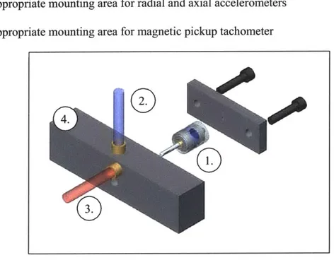
Figure 10: Exploded view of testbed setup: 1. Turbine canister 2. Inlet air path 3. Exhaust air path 4. T est block... 26

Figure 11: Schematic of experimental setup: Front view showing lateral and axial

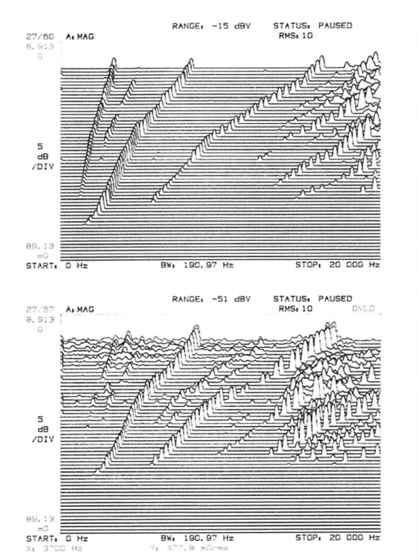
accelerometers, magnetic pickup, and the low-stiffness open cell foam base... 28 Figure 12: Waterfall plot showing (a) lateral acceleration and (b) axial acceleration for

rotor with Viton -70 bearing supports. X-axis represents the frequency domain: 0 Hz - 20 kHz. Y-axis represents the changing rotor speed: speed range 9,600 rpm -345,000 rpm. Acceleration is measured on the Z-axis: OG - 8.913G... 34

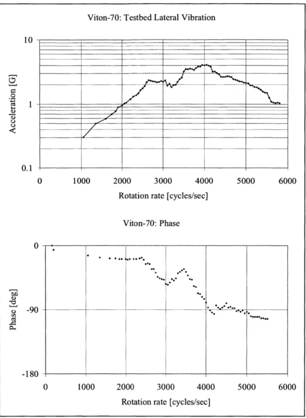
Figure 13: Vibration and phase of testbed, measured in the lateral direction. Phase

m easured relative to shaft tachometer... 35

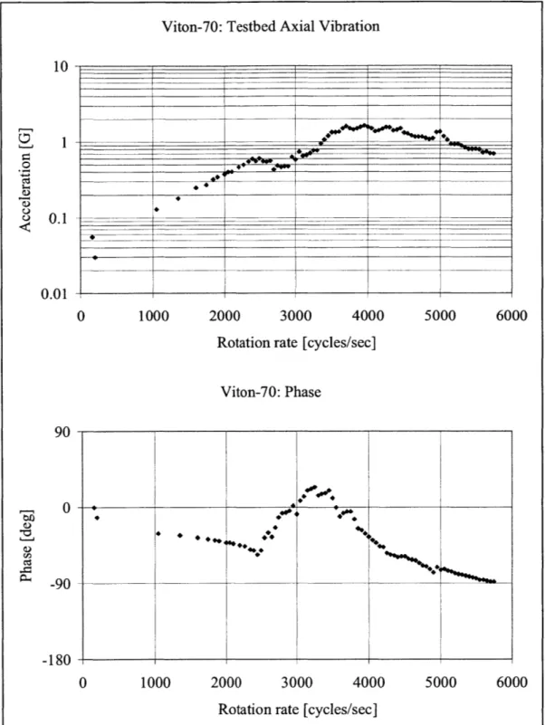
Figure 14: Vibration and phase of testbed, measured in the axial direction. Phase

m easured relative to shaft tachometer... 36

Figure 15: Buna-N 0-ring after testing and disassembly. Black debris resulted from the disintegration of flash during turbine operation... 38

Figure 16: Waterfall plot showing (a) lateral acceleration and (b) axial acceleration for rotor with Buna-N bearing supports. X-axis represents the frequency domain: 0 Hz

- 20 kHz. Y-axis represents the changing rotor speed: speed range 4,800 rpm

-480,000 rpm. Acceleration is measured on the Z-axis: OG - 5G... 39 Figure 17: Vibration and phase of testbed, measured in the lateral direction. Phase

m easured relative to shaft tachometer... 40 Figure 18: Vibration and phase of testbed, measured in the axial direction. Phase

m easured relative to shaft tachometer... 41 Figure 19 Waterfall plot showing (a) lateral acceleration and (b) axial acceleration for

(6)

- 20 kHz. Y-axis represents the changing rotor speed: speed range 3,960 rpm -492,000 rpm. Acceleration is measured on the Z-axis: OG - 2G... 43 Figure 20: Vibration and phase of testbed, measured in the lateral direction. Phase

m easured relative to shaft tachom eter... 44 Figure 21: Vibration and phase of testbed, measured in the axial direction. Phase

measured relative to shaft tachom eter... 45

Figure 22: Voigt viscoelastic model with stiffness and damping coefficients. (Atkirk and G oh ar 187) ... 4 7 Figure 23: Comparison between two curve-fits for estimation of dynamic properties of

Viton*-70 elastomer. (a) Stiffness (b) Loss Coefficient... 50 Figure 24: Modeshapes and modal frequencies for rotor with Viton*-70 bearing supports.

... 5 1

Figure 25: Bode plot of undamped response to imbalance for rotor with Viton®-70

bearing supports... 5 1 Figure 26: Bode plot of response to imbalance of rotor with Viton*-70 bearing supports.

Model incorporates damping estimates provided by Atkurk and Gohar... 52 Figure 27: X-Y plots and transient motion of shaft center, rotor with Viton* 70 bearing

supports, modeled at 25'C, and incorporating damping estimates developed by Atkurk and Gohar. (1) 190,000 rpm: Below first rigid-body critical speed. (2)

360,000 rpm: Near first rigid-body critical speed. (3) 500,000 rpm: Above first

rigid-body critical speed. Rotor achieves limit-cycle (stable) motion at all speeds w ithin norm al operating range ... 53

Figure 28: Whirl mode shapes of rotor with Viton*-70 bearing supports. Backward whirl at 190,000 rpm and 500,000 rpm indicate too high a level of predicted damping in finite elem ent m odel. ... 54 Figure 29: Rotor system with Viton*-70 bearing supports (a) Stability map (b) Whirl

speed map showing damped natural frequencies... 55 Figure 30: Transmitted force at bearing 1 and 2 for rotor with Viton*-70 bearing

su p p orts... 56

Figure 31: Comparison chart of thermal conductivity of Viton*, Buna, and silicone elastom ers versus other m aterials. ... 58

Figure 32: Temperature dependence of elastic modulus of Viton*-70 according to

Sm alley, D arrow , and M ehta ... 58

Figure 33: Bode plots for imbalance response of rotor with Viton*-70 bearing supports;

66 'C case. (a) Undamped (b) Damping provided as measured from experimental

re su lts. ... 5 9

Figure 34: Finite element analysis of rotor model with Viton*-70 bearing supports. (a) Whirl speed map indicating damped natural frequencies at 231,000 rpm and 444,000 rpm. (b) Stability map indicating stable rotor behavior... 59

Figure 35: Finite element analysis of rotor model with silicone bearing supports. (a) Whirl speed map indicating damped natural frequencies at 120,000 rpm and 200,000 rpm. (b) Stability map indicating stable rotor behavior up to 480,000 rpm. ... 63 Figure 36: Shaft center motion of rotor with silicone bearing supports. (a) Stable,

limit-cycle motion at 200,000 rpm (b) Unstable elliptical motion at 500,000 rpm... 63 Figure 37: Bode plot of axial vibration of rotor, showing system eigenvalues... 65

(7)

Figure 39: Accelerometer calibration certificate ... 71

Figure 40: Magnetic pickup (tachometer) specifications... 72

Figure 41: Frequency-dependent elastic and loss moduli of Buna elastomer, referenced to elastic modulus of Viton-70. Predictions based on Smalley, Darrow, and Mehta. .73

Figure 42: Dynamic force/deformation properties of natural rubber, illustrating different regions of material behavior. (Source: Freakley 68) ... 74 Figure 43: Dynamic Elastic and Loss Modulus for Viton B (durometer 75±5) (Source:

Jon es 4 4 ) ... 7 5

(8)

List of Tables

Table 1: Stiffness and loss coefficients for power law estimation of Viton-70 dynamic material properties. (Smalley, Darlow, and Mehta 3-25) ... 47 Table 2: Damping values for Viton®-70, based on half-power method applied to

experim ental data... 49 Table 3: Model coefficients for frequency-dependent stiffness of silicone elastomer... 62 Table 4: Model coefficients for frequency-dependent damping of silicone elastomer. ... 62

(9)

Chapter 1: Background

1.1 Introduction

High speed air-impulse turbines power a multitude of devices, including tools found in odontology, medicine, and art. The miniature impulse turbines attain speeds exceeding 400,000 rpm. Vibration and noise are common characteristics of these rotors, creating at the least, an annoyance, and at the worst, a hazardous ergonomic environment (Dyson

219-232).

A typical medical drill is illustrated in Figure 1. The typical air driven drill uses a

high pressure (30-35 psi) air source to drive an impulse turbine, which spins on rolling element bearings. The rotor/bearing assembly is isolated from the housing by

elastomeric 0-rings.

drive air pipe pre-load spring

(30-35 psi) _{O-ring bearing supports,,,_,.,,,}

airflow

handpiece exhaust pipe

impulse turbine

ball-bearings _{bit (1/16 in.)}

Figure 1: Schematic representation of a typical high-speed turbine and its housing.

Operation of the typical high speed air drill involves a very short startup transient, followed by a few seconds of work, and finally a short run-down to rest. Typical high-speed rotors spin at high-speeds between 350,000 - 450,000 rpm. Vibration at steady-state is

9 ... .... ... .. .. .. ....

(10)

usually dominated by the once-per-revolution signal between 5.8 kHz and 7.5 kHz. The most common cause for once-per-revolution vibration spectra is imbalance in the rotor. In addition to the vibration at rotation rate, several other key frequency multiples are common, including frequencies typically associated with the rate of ball-bearing retainer-pass, as well as misalignment in the bearings.

Regardless of the particular spectral content during the operation of the rotor, the severity of vibration is largely frequency-dependent. Since the rotor-bearing system is compliantly supported, the system can be modeled as multiple degree of freedom

mechanical system, possessing fundamental frequencies which amplify the response to an input disturbance. Understanding the frequency response of the rotor is critical to the optimization of its dynamic behavior.

1.2 System Components

A typical rotor-bearing and shaft assembly is shown in Fig 2:

Figure 2: A typical high-speed air driven impulse turbine. The aluminum rotor has an outside

diameter of 0.295". The rolling element bearings have an outside diameter of 0.25". The shaft is 0.0625" diameter stainless steel. Each bearing is supported by an O-ring with a cross-section of

(11)

1.2.1 Bearings

High-speed impulse turbines of this type have been historically supported by either air bearings or ball bearings. However, ball bearings have increasingly replaced air bearings as the antifriction device of choice because of their ability to supply higher load capacity, and the resultant resistance to stall. Also, ball bearings enable the use of lower supply air pressures, and tend to be more stable than air bearings (Dyson 15). Finally, the

high level of precision available in ball bearings, at a low price, has further displaced air

bearings as a choice in high speed turbines.

1.2.2 Rotors

Turbines extract potential energy from a fluid. Turbines can be classified as one of two types: reaction or impulse (White 742-748). Reaction turbines are low pressure, large flow devices. The turbine vanes possess a hydrodynamic shape which reacts with a fluid stream to provide lift, which in turn causes rotation of the turbine around a shaft. Impulse turbines are momentum-transfer devices, in which a high-velocity jet of fluid, at atmospheric pressure, impinges upon the turbine blade, causing rotational motion. Both reaction and impulse designs have been used in high speed air driven machinery, but according to Dyson, the impulse turbine is the most commonly used design today (16). A wide range of blade designs have been proposed for use in impulse turbines. Some of the most common have been illustrated in Figure 3. Despite the variations in blade design, no reliable evidence has shown significant advantages to any particular design (Dyson

19). The difference appears to be driven mainly by market differentiation between

(12)

(a) (b) (c) (d)

Figure 3: Common impulse turbine designs include (a) flat blade (b) double curved (c) simple curved (d) split cup

Given the high rotational speed of operation, balancing is critical to smooth operation of these rotors. Thus, many rotor/bearing assemblies are dynamically balanced as part of the manufacturing process. Dynamic balancing involves the removal of

material from the rotor blades to bring the mass center of the rotor/bearing assembly close to the axis of rotation of the assembly (Ehrich 3.1-116). The rotor and bearings are often supplied as a completely assembled "cartridge" to minimize the possibility for an unbalanced turbine.

1.2.3 Vibration Isolation Methods

Vibration has been a major concern in the operation of high speed air-driven turbines. If the mass center of the rotor/bearing assembly does not coincide with the center of rotation, then an oscillatory force will be induced which is proportional to the square of the speed of operation:

Fnbalance = munbalancer C2 Equation 1

where r is the distance between the mass center and the center of rotation, and (o is the rotation rate in radians/sec.

(13)

Dynamic balancing is the method of choice to reduce the vibration level in high speed air turbines. However, some small level of remaining imbalance is inevitable, so a means of vibration isolation has been adopted to allow the rotor to rotate about its center of mass. Elastomeric O-rings, mounted on the outer surface of the bearings, have been commonly used to provide lateral vibration isolation. Axial vibration isolation has been provided either by O-rings, or by wavy washers. Common elastomers chosen for this task include Viton*, Buna-N, and silicone.

Viton® is a fluoroelastomer known for its resistance to heat and for its high damping properties. Buna-N, or perbunan, is a copolymer of butadiene, natrium (sodium), and acrylonitrile. It is known for its resistance to oils, but has lower heat resistance than Viton®. Silicone is known for its extreme temperature range, but it has

lower damping properties than either Viton® or Buna-N (Freakley 15-18).

Elastomers are commonly rated by the Shore A hardness system, which is a means of classifying the hardness of a material under a point load. Currently, most high speed turbines are supported by elastomers with a durometer of 65-70.

Powell and Tempest have noted that Viton® and silicone O-rings are effective in the suppression of whirl in a turbine supported by air bearings with rotation rates of up to

110,000 rpm. The authors noted that in general, increasing temperature and hardness of

the elastomer both tended to reduce the effectiveness of whirl suppression (705-708). Atktirk and Gohar have also noted that O-rings are effective in vibration isolation. In a turbine whose maximum rotation rate was 60,000 rpm, Viton* was shown to be effective in reducing vibration amplitudes. Viton*-70 was shown to be more effective than Viton®-90, in part because its damping coefficient was larger (187-190).

(14)

Bearing support stiffness has been shown to be important in the design of smooth-running rotational machinery. Specifically, the choice of support stiffness can affect the placement of rotor fundamental frequencies (Gunter 59-69, LaLanne and Ferraris 141, Ehrich 1.2). As noted by Atkurk and Gohar, an understanding of the dynamic

characteristics of O-rings is critical to their successful use in rotating machinery

(189-190). Most data on dynamic material properties exists in the 1 - 1,000 Hz frequency

range, largely because most industrial applications of rubber are low-frequency (Freakley

319). In addition, high frequency measurements of rubber are considerably more difficult

to perform than low-frequency measurements (Smalley, Tessarzik, and Badgley

121-131). Some attempts to predict the behavior of elastomers in the frequency range of

1,000 Hz - 10,000 Hz, corresponding to shaft speeds of 60,000 rpm - 600,000 rpm, have

been made, but little real-world verification in studies on actual machinery exists (Jones

37-48).

Elastomers exhibit major changes in material properties with changes in

environmental variables such as vibration frequency and temperature (Freakley 56-109, Payne 25-33). The degree of change in material property varies between elastomers, yet little literature exists to justify the choice of a certain elastomer for the O-ring bearing supports in current high speed air turbine designs.

The specification of O-rings as components in precision machinery has been controversial because of their loose manufacturing tolerances. According to AS568 0-ring standards, the width of O-0-rings with cross sections of 0.030" are held in the ± 0.003" range, whereas diametrical tolerances on bearings and other steel components are held to less than 0.0002" (eFunda website). However, as is noted by Powell and Tempest,

(15)

0-rings are produced in batches, and dimensional variance within a batch is often less than

0.001"; the larger dimensional tolerance is a cross-batch specification (705). By

choosing O-rings from the same batch, dimensional precision can be improved. O-rings have been shown to be effective in vibration isolation and damping applications, but a need exists for better quantification of their performance.

1.4 Thesis Structure

Chapter 2 develops analytical techniques relevant to modeling of dynamics of the

high speed rotor. Chapter 3 describes the experimental setup and outlines the

experimental method for the parametric study of several flexible bearing support

schemes. Chapter 4 presents and discusses experimental and analytical results. Chapter 5 brings the thesis to conclusion, and evaluates the overall success of the project in light of the hypothesis. In addition, some recommendations for future work are given.

Chapter 2: Theory

To completely describe the motions of the single-span rotor, six degrees of freedom are required: the three translational motions x, y, z and the three rotational motions of the rotor mass center, which can be interpreted as roll, pitch, and yaw. The general equations of motion are highly nonlinear and are difficult to solve analytically. However, these equations may be simplified by assuming constant angular velocity, small bearing displacements, and zero axial motion. Thus, the total number of degrees of freedom is reduced from six to four; including the two translational (x, y) and two

(16)

y

x

0 X

Figure 4: Schematic of rotor model with reduced degrees of freedom.

We are interested in the forced response of the rotor. Assuming perfect rolling element bearings, the forcing function for the spinning rotor can come from relative misalignment between the bearings, aerodynamic cross-coupling between the turbine blades and the housing, and most commonly, static and/or dynamic imbalance in the rotor.

Static imbalance occurs when a "heavy spot" on the rotor causes a periodic force to be exerted perpendicular to the axis of rotation. Dynamic imbalance results from two or more non-coplanar "heavy spots" interacting to create a wobbling forcing function.

A rotor's response to imbalance will be characterized by a number of critical

frequencies, or mode shapes. The first two critical speeds are rigid-body modes, especially since the rotor's stiffness is large compared to the support stiffnesses. As is shown in Figure 5, for a symmetrically suspended rotor on infinitely flexible mounts, the first and second mode shapes are cylindrical whirl and coning, respectively. The first flexible rotor critical is the third modeshape.

(17)

N YA1 Mtkdenne flexdi.hty Infinite fQci jfl Mod_

Figure 5: Modeshapes of simply supported shaft with varying levels of support flexibility relative to

shaft stiffness. With flexible bearing supports, first and second modes are rigid-body modes. (Source: Handbook of Rotordynamics, Fredrich F. Ehrich)

2.1 Finite Element Analysis

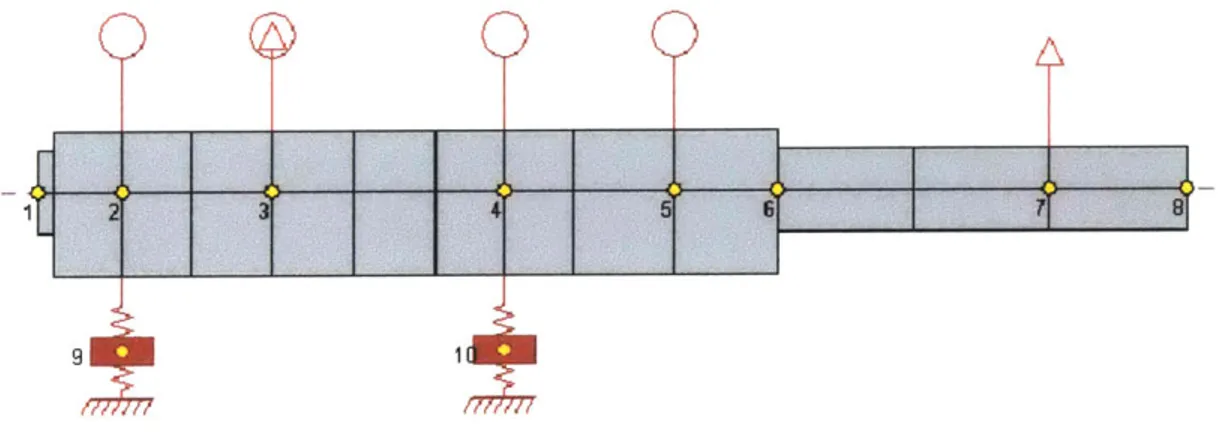
Implementation of a finite element model provides the most detailed analysis of the dynamics of the rotor. The rotor can be modeled as a series of shaft elements and rigid disks (Figure 6). A third-party software package -DyRoBes: Dynamics of Rotor Bearing Systems -was used to construct the FE model.

1 6

9t 1

Figure 6: Finite element model of high speed air-driven turbine. 7 shaft stations with 13 substations.

Two imbalances 180' apart on shaft. 4 lumped inertial stations.

17

(18)

-The rotor model consists of 7 shaft stations with 13 substations. -There are 4 degrees of freedom at each substation. The turbine is modeled as a rigid disk centered between the bearings. The inner rings of both ball-bearings are also modeled as rigid disks, to capture their contribution of inertial effects at high speeds. A dynamic

imbalance is included in the model following manufacturing tolerances which hold the rotating imbalance to less than 4.OE-6 oz-in. Thus, an unbalance of 6.477E-10 Lbf-sec2

is placed at the turbine. A static imbalance of 5.057906E-15 Lbf-sec2 _{was added at the}

end of the shaft to simulate the imbalanced bit used in testing. The wavy preload washer is modeled as an axial stiffness of 50 Lbf/in. The rotor supports were modeled as flexibly supported rolling element antifriction bearings. The bearing stiffness coefficients

account for the nonlinear dynamic behavior of the elastomeric supports.

To simplify the modeling process, a number of assumptions were made. First, all elements, including the rotor and its flexible supports, are assumed to be axisymmetric. The outer bearing ring is assumed to be a rigid body, since it is considerably stiffer than the flexible supports. Moments of inertia of the shaft are calculated at discrete intervals and lumped at the finite element stations. The shaft is modeled with separate mass and "stiffness radii" to enable accurate calculation of shaft modeshapes while correctly representing the inertial behavior of the rotor at very high speeds. The inertia of the balls and retainer are neglected in the model, but their masses are included in the mass of the shaft so that the total vibratory mass amount is correct. The O-ring bearing supports are modeled as speed-dependent bearing elements, while the rolling element bearings are treated as linearly stiff support elements. This assumption is justified by the high and relatively linear stiffness behavior of ball bearings compared to elastomers.

(19)

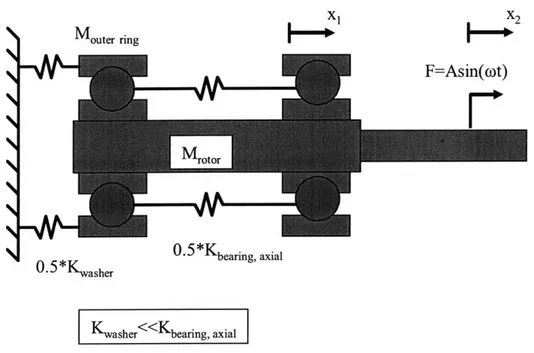
2.2 Axial Vibration

The rotor/bearing assembly can be modeled as a two degree-of-freedom oscillatory system (Figure 7). x₂ xl

H-*

M ring 0.5*Kwasher 0. 5_{*Kearing, axial}

Kwasher Kbearing, axial

Figure 7: Schematic representation of rotor/bearing assembly for axial vibration modelling.

Damping is minimal in this system. The equations of motion are:

mouterring 1 + (kwasher± kbearing ) ₁-kbearing X2 = 0

Mrotori2+ kbearing X2 -kbearingXi = f(t)

Written in matrix notation:

Mouter _ring

0

0 1 1 kwasher bearing bearing X

-m, _ ₂_ -kbearing kbearing [X _{2 _} f(t)) Mi+ Kx = F Equation 2 Equation 3 or Equation 4 Equation 5 Is

(20)

The homogenous solution is found by settingf(t) = 0. Assume that Equation 5

has the harmonic solutions:

x(t) = ek _j k Xj ckke )kt k =1,2 Equation 6

X2k

where Xk is the mode shape and (Ok is the modal frequency. Substitution of Equation 6

into Equation 5 yields:

M( cok 2 ktce' + K(cke')' =0 Equation 7

MK-

Mo4k =

0

Equation 8

Fkahe+ k 2i -k

washe, beainng otkeg bearing 2 Ilk =[G(O)XX)=o0 _{Equation 9} kbeang kbearing Moto, W k] X2k

The matrix [G(wk)] must be singular for a nontrivial solution to exist. In other words:

G( iouterring bearing O( - (kbearmng ,outerring + (kouter ing+ kbearing )lfbearfng )t2+ kouter ring keaing =0

Equation 10

This is known as the characteristic equation of the system. As a quadratic, the solutions co, and 92 can be found by solving the quadratic formula. These solutions are the natural frequencies, or modal frequencies, of the system. Knowing the natural frequencies, the mode shapes can be determined. The mode shapes are defined as the amplitude and directions of the reactions xj and x2 when the system oscillates at the

(21)

X h= 1 " J e' + l 12 C2)e = ₁ c sin(cwt + , )+ X2c, sin(co2t +$2) Equation 11 (X21 )(X22

where c], c2,

#

, and

#2

are constants determined by the initial conditions x(O) and i(o).

Thus, the mode shapes and modal frequencies can be calculated for the 2 degree-of-freedom model for the axial vibration of the rotor.

Chapter 3: Experimental Methods

Experimental verification of the dynamic behavior of high-speed, miniature turbines presents a major challenge to laboratory instrumentation. Direct and indirect measurements of vibration parameters (displacement, velocity, and acceleration) are possible on the rotor system.

3.1 Sensors

The rotor and bearings are concealed by a housing, and are inaccessible to direct measurement. The only part of the system accessible to a direct vibration measurement is the protruding shaft. A capacitive measurement system was available, the ADE

MicroSense 3401, which was capable of measuring the 1/16" shaft. However, because of limitations imposed by the need to measure the rotor/bearing system in an unconstrained environment (discussed in section 3.3), the use of the capacitance sensor was prevented.

Vibrations of the housing result from a transfer of force from the rotor;

measurement of vibration on the housing provides an indicator of rotor vibration severity. In addition, insight into acoustic properties of the rotor is gained by an understanding of the housing motion. Vibration of the housing is conveniently measured with

(22)

1 Omv/G to 1 00mv/G. High sensitivity accelerometers provide better signal-to-noise ratios, but at a high price . After preliminary exploration, a small form-factor, IOmV/G piezoelectric accelerometer was found to provide satisfactory performance, after coupling with an external amplifier.

Speed measurement of the shaft was accomplished using a magnetic-pickup sensor, after consideration of several alternatives, including optical sensors and acoustic methods.

Optical tachometers depend on the ability of a photon emitting-and-receiving pair to sense changing patterns of light and darkness. Fiber optic sensors are very suitable for high frequency measurement because of their fast response time of ~0. 1 ps to 1 ps.

However, cost and configurability precluded the use of a fiber optic system.

Acoustic methods have been suggested for speed measurement, since high speed air impulse micro-turbines exhibit a characteristic "whine", which, at rotation speeds above 75,000 rpm, is largely due to synchronous (once-per-rotation) spectral content caused by rotor imbalance. With bandwidth filtering, a prediction of rotation rate can be

inferred by audible frequency content. However, this method has been shown to have high uncertainty, with accuracy limited to t1,000 rpm (Dyson 95). Also, spurious

acoustic components, due to a variety of causes, may corrupt the prediction. Finally, acoustic methods of speed prediction eliminate phase information from the data set, further reducing their usefulness in data analysis.

Magnetic pickups sense fluctuations in magnetic impedance. When a keyway or a flat is introduced to a shaft, the magnetic pickup will produce a sinusoidally varying output voltage, which is indicative of the rotational rate. The output voltage of the

(23)

magnetic pickup is inversely proportional to the square of the distance to the target, and proportional to the rotation rate. With an air-gap of 0.005", the sensor provides 0.6V peak-to-peak at 30,000 rpm. The magnetic pickup method was chosen as the best combination of robustness, price, and performance for this project.

3.2 Flexible bearing supports

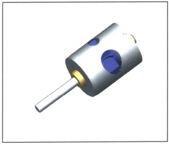
The turbine chosen for this study is a high-speed air impulse turbine with simple cup geometry. The turbine is a commercial model, and has the unique characteristic that the rotor/bearing assembly is packaged within a steel canister (Figure 8). This has the effect of removing some uncertainty of interaction between the rotor/bearing assembly and the housing, assuming manufacturing controls on the canister and rotor assemblies are good. Also, the canister form factor is convenient for experimentation, because it allows simple test-bed geometry.

Figure 8: Solid model of canister-type high speed air driven turbine assembly.

23

7/00

(24)

--Each bearing in the test turbine bearing pair is supported by a single elastomeric O-ring. Thus, to change the support stiffness, O-rings of identical dimensions, but different material properties, were tested. Three different materials were selected for this parametric study: Viton*-70, Buna-N, and silicone, each with a durometer rating of 70. Each of these materials has been previously used commercially as a bearing support in this application. However, the most common elastomer choice is Viton*-70, most likely because of its high damping ability and its ability to withstand high temperature medical

autoclaving.

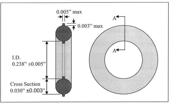
O-rings for the study were purchased from Apple Rubber, Inc. The specified dimensions exactly matched the stock O-ring dimensions of 0.030"CS x 0.298"OD, with a 0.003" tolerance on the cross-section. However, one major difference between the different O-rings concerns the matter of "flash". Flash is an artifact of the O-ring

manufacturing process. It consists of a raised portion of material on the ID and OD, left

by the two halves of the O-ring mold (Figure 9). Two of the elastomeric O-rings in this

study -Silicone and Viton* - were de-flashed; the flash was removed in a cryogenic

post-manufacturing operation. To cryogenically de-flash an O-ring, the product is frozen, and then the flash is broken off of the body, and the surface is ground flush. The flash

(25)

Figure 9: Schematic of 0-ring, showing flash dimensions.

Taking advantage of the convenience of the canister-type design for experimentation, four canister-type turbines were disassembled and retrofitted with new (different) O-rings for a different bearing support. The procedure to retrofit a turbine is:

1. Place canister into turbine press. 2. Gently apply force to axle.

3. After canister cap "pops" off, release force.

4. Separate canister cap from canister body, and remove rotor/bearing assembly. 5. Using needle, pick out old O-rings from canister cap and body.

6. Lubricate new O-rings with Minapore Light Oil. 7. Replace 0-rings.

8. Re-seat rotor/bearing assembly into canister body. 9. Align canister cap with canister body, under press. 10. Gently press canister cap onto body.

0.005'" max A 0.003" max A I.D. 0.238" ±0.005" Cross Section 0.030" ±0.003",

(26)

3.3 High-speed rotor test-bed

The test-bed was designed to study radial and axial vibrations caused by the rotor under its full operating speed range. Under normal operating conditions, air is forced at up to

35 psi through a converging nozzle to drive the impulse turbine, while exhaust air escapes out large diameter orifice to the room.

Conditions for the test-bed are:

" high structural stiffness

* appropriate mounting area for radial and axial accelerometers

" appropriate mounting area for magnetic pickup tachometer

3.

Figure 10: Exploded view of testbed setup: 1. Turbine canister 2. Inlet air path 3. Exhaust air path 4.

Test block

A rigid steel block, with a cavity for the turbine canister and appropriate air path

fittings, was chosen as an appropriate form factor for the test-bed (Figure 10). The natural frequency of the block is calculated with Rayleigh's method on a lumped

parameter model of the block. First, the block is modeled as a simply supported beam of

(27)

length L. A force, P, equal to the weight of the block, acts on the center of the beam. The deflection of the beam is:

-Px3L 2 _{_4x} 2)

J(x)=

48EI S=P(LxXL2 - _8xL+4x2) 48E1 L 2 2 < x < L 2 where I is the area moment inertia of the beam:

bh3 12

The maximum deflection of the beam is:

max = = - = -2.09 x 10 7'in

4-2 48EI

Rayleigh's method solves for the natural frequency of the beam by equating the kinetic and potential energies of the system. The potential energy, in the form of strain energy in the deflected shaft, is maximal at the largest deflection. The potential energy is defined as:

E

= K(m3a)₂ Equation 15

The beam is assumed to undergo sinusoidal motion, due to an external excitation. The kinetic energy is maximum when the vibrating shaft passes through the un-deflected position with maximum velocity. The kinetic energy is defined as:

Ek - Wn" (M2)

2 Equation 16

Equation 12

Equation 13

(28)

Setting Ep=Ek yields:

Co, = g_: =

-54,270.09Hz

m - 3max

Equation 17

The block's resonant frequency is extremely high, so the test-bed dynamics will not interfere with the rotor. To ensure the free motion of the test-bed, the block is mounted on a sheet of open cell foam (Figure 11).

Testbed]

-Accelerometers

Magnetic Pick-up

Open Cell Fa

Figure 11: Schematic of experimental setup: Front view showing lateral and axial accelerometers, magnetic pickup, and the low-stiffness open cell foam base.

The procedure for setup of the test-bed is as follows:

1. Release the back-cap by removing screws.

2. Remove any prior turbine canister from the test-bed

3. If a specific test bit is being used, install it into the new turbine chuck.

4. Place turbine canister to be tested into the cavity; align ball with groove to ensure proper orientation of airways.

(29)

The block is fitted to accept standard "push-to-connect" plastic airline couplings. The drive air port is supplied by 6mm plastic tubing, whereas the exhaust is created with a 24-inch section of 8mm tubing. This length of tubing is used, instead of directly exhausting the air to the atmosphere, because it was found that porting the exhaust improved the stability of the turbine performance. A manual checkvalve regulates airflow to the turbine, allowing the air pressure to be varied from 0 psi to a line maximum of >60 psi.

3.2 Spectral analysis with parametric bearing support variation

Frequency-dependent rotordynamic characteristics of low mass, high speed turbines are often masked by the extremely fast start-up time of the impulse turbine, when operated at the normal operating air pressure of 35 psi. However, variation of input air pressure can reveal the transient response. Specifically, we are interested in the synchronous response and its harmonics, spectral content related to ball bearing frequencies, as well as non-frequency dependent spectral content, such as structural resonances.

To discover the frequency behavior of the rotor, the input air pressure was varied, causing the turbine to spin at a series of steady speeds ranging from 0 rpm to the

maximum attainable speed; usually around 500,000 rpm. Approximately 70 discrete steady state speeds were recorded for each canister, with an average step size of 6,500 rpm. A combination of sensors, digital lab equipment, and computers was used to analyze the vibration data from the test-bed. Signals from accelerometers in the radial and axial directions were first passed through a Bruel & Kjaer Model 2525 DeltaTron amplifier, to boost the signal to noise ratio. The improved signals, as well as the tachometer signal, were monitored on a Tektronix TDS 1012 oscilloscope. The

(30)

acceleration signals were then passed to a Hewlett-Packard Model 3561A single-channel digital spectrum analyzer (DSA) which collected up to sixty sequential samples to create a cascade plot. Each accelerometer signal was then compared to the tachometer input for a phase measurement, using a Hewlett-Packard 8562A two-channel digital spectrum

analyzer. An RMS average of 16 samples gave the phase between the tachometer and the acceleration output, and this value was recorded by hand. In addition, the peak

magnitude of the acceleration was recorded in Excel for each sample. The procedure to test a canister is:

1. Mount canister inside of test-bed as described above.

2. Adjust air pressure to 35 psi, or to a level that yields a rotational frequency of 6.5 kHz (or 390,000 rpm).

3. Run turbine for 2 minutes at 390,000 rpm to warm up bearings and distribute

lubricant.

4. Reduce air pressure to the minimum needed to stably actuate the turbine. This is usually 6 psi - 8 psi.

5. Properly scale oscilloscope, DSA's.

6. Record shaft rotational speed as indicated by tachometer signal.

7. For radial accelerometer, record vibration amplitude given by B&K 2525. 8. Record phase for radial accelerometer, from dual-channel DSA.

9. Add a sample to the cascade plot on the DSA 356 IA. 10. Repeat for axial accelerometer.

11. Increase speed by -5,000 rpm and repeat Steps 1-10.

(31)

Chapter 4: Results and Discussion

4.1 Experimental Results

This section describes and discusses the response of the rotor to unbalance forces when operated across its entire speed range from 0 rpm -400,000 rpm. The effect of

substitution of various elastomers for the bearing supports is presented.

Spectral analysis of waterfall plots of the rotor response reveal frequency dependent behavior related to the rotor and bearing dynamics. In particular, strong components of the spectra include vibration at the rotation rate (IX), twice the rotation rate (2X), and at the rotation rate of the ball bearing retainer. Ball bearings have unique vibration characteristics, related to geometry and rotation rate. The major characteristic frequencies are:

RPM _ RPM

Fundamental train frequency: RPM 1 - cos(#) ~ (0.3987)

60 2 D 60

Defect on outer race: RPM 1 cos() ~(0.3987) RPM

60 2 D, 60

RPM n D RPM

Defect on inner race: - 1+ Db cos(#) (4.2090) 60

60 2 DP 60

RPM D rD1 RPM_

Ball defect frequency: D- Il- cos2(0) = (4.6621) RPM

60 Db D 60

Equation 18

Equation 19

Equation 20

(32)

where Db is the ball diameter, Dp is the pitch diameter, O is the contact angle in degrees, and n is the number of balls in the bearing. For the bearings involved in this study, Db

-0.03937 in., D = 0.1914 in., #= 10, and n = 7 balls.

4.1.1 Viton*-70

Turbine serial number 2J0213 incorporates Viton® O-rings for its bearing supports. Since Viton* is the material specified as an "Original Equipment

Manufacturer" (OEM) part, this turbine was not disassembled before testing. The rotor was operated from a minimum speed of 9,600 rpm to a maximum speed of 345,000 rpm.

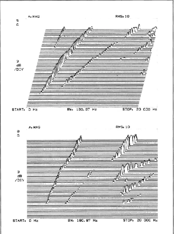
Spectral analysis of lateral and axial vibration reveals the existence of rotor resonances, as well as complex behavior related to ball bearing dynamics (Figure 12). Prominent vibration is detected at IX rotation rate, which is a result of the imbalance in the rotor. Vibration at twice the rotation rate (2X) begins to appear at 3,200 rpm and is prominent for all higher rotation rates. Vibration at the fundamental train frequency (FTF) appears at 3,250 rpm, and grows somewhat linearly as the rotation rate is

increased, possibly indicating some energy interaction at the cage/ball interface. Other vibration components exist at non-integer multiples of the rotation rate, but are not

characteristic ball bearing frequencies. Spectral components that are unrelated to rotation rate also appear, indicating structural resonance or possibly looseness. For instance, a broad amplification region exists for axial vibration in the range of 14,500 Hz to 18,500 Hz. This amplification effect is not noticed in the lateral vibration measurements. Instead, some high frequency amplification exists for lateral vibration above 18,500 Hz;

(33)

Vibration at the lX frequencies displays non-linear behavior. Lateral acceleration levels increase from OG through a broad peak to 4.07G at 4,050 Hz, or 243,000 rpm, after which the vibration level reduces to about 1G. The phase of the lateral acceleration relative to the rotation of the shaft lags by 90* at 4,050 Hz.

(34)

RANGEt -15 dBV STATUSs PAUSED

2' 63 A& MAG RMSs 10

d6

/DIV

STARTv 0 Hz SW* 190.97 Hz STOP2 20 000 Hz

RANGE -51 dBV STATUS PAUSED

A&MAG RMSs 10

d8 /D IV

START 0 Hz SWr 190. 97 Hz STOPs 20 000 Hz

Figure 12: Waterfall plot showing (a) lateral acceleration and (b) axial acceleration for rotor with Viton®-70 bearing supports. X-axis represents the frequency domain: 0 Hz - 20 kHz. Y-axis

represents the changing rotor speed: speed range 9,600 rpm - 345,000 rpm. Acceleration is measured on the Z-axis: OG - 8.913G.

(35)

Viton-70: Testbed Lateral Vibration

10

1

0.1

0 1000 2000 3000 4000

Rotation rate [cycles/sec]

5000 6000 Viton-70: Phase 0 -90 -180 0 1000 2000 3000 4000

5000 6000

Figure 13: Vibration and phase of testbed, measured in the lateral direction. Phase measured relative to shaft tachometer.

0 0 0 C) C) * *.4 ***44** *4 4. 444*44444

(36)

Viton-70: Testbed Axial Vibration ____________ 4 4 _______________ _______________ _______________ II _ 4 4 2000 3000 4000

Viton-70: Phase

2000 3000 4000

Figure 14: Vibration and phase of testbed, measured in the axial direction. Phase measured relative to shaft tachometer. 10 1 0.1 0 C) 0.01 0 1000 5000 6000 90 0 -e 0 0 -90 *4 * 4.. .4. 4 4 ** 4 * 4 44 444.4 4 4 -180 0 1000 5000 6000

(37)

4.1.2 Buna-N

Turbine serial number 2K034 incorporates Buna-N 0-rings for its bearing supports. This turbine was disassembled before testing in order to replace the original (Viton -70) O-rings with the Buna-N elastomer. The rotor was operated from a minimum speed of 48,000 rpm to a maximum speed of 480,000 rpm.

Prominent vibration is detected at IX and 2X rotation rate. The 2X component begins to appear at 28,000 rpm and is small relative to the IX component until the rotor speed reaches 432,000 rpm. This rotational rate (7,200 Hz) places the 2X component at 14,400 Hz, where a broad resonant region is excited. This phenomenon is present in both lateral and axial vibration spectra, but is stronger in the axial data, where a broad

amplification region exists for axial vibration in the range of 14,200 Hz to 17,000 Hz. Vibration at the FTF appears only in the lateral vibration data, becoming noticeable at

375,000 rpm. The small component of vibration due to the FTF indicates low energy loss

at the cage.

Vibration at the IX frequencies displays non-linear behavior. Lateral acceleration rise abruptly to 3.3G at 3,300 Hz, drop rapidly to 1.6G at 3,500 Hz, and then gradually

increase through a broad peak to 3.5G at 4,000 Hz, or 240,000 rpm. After this point, the vibration level reduces to 1.6G at 342,000 rpm, and finally increases to 3G at 480,000 rpm. The phase of the lateral acceleration relative to the rotation of the shaft lags by 630 over the entire operating range.

The rotor on Buna-N bearing supports exhibited very high levels of axial vibration, both in respect to its own lateral vibration levels, and to the axial vibration levels from the rotors with Viton-70 and silicone supports. This may be due to the effect

(38)

of flash remaining on the O-ring, which tended to impart destabilizing forces on the bearing rings.

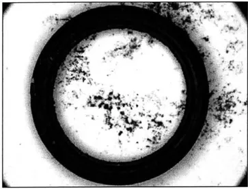
The flash on Buna-N bearings is a result of the manufacturing process; it is actually the parting line on the O-ring, left over from the mold. After running the turbine with Buna-N rotor supports, the system was disassembled and inspected. A large amount of black debris was found inside the canister (Figure 15).

Figure 15: Buna-N 0-ring after testing and disassembly. Black debris resulted from the disintegration of flash during turbine operation.

(39)

5

dE

E TARTa Z zRO ~~ zSOS~ COO Hz

MAG R?4Sv 10

D/~ V

SToARTs 1) HZ Y IW 90. 97 Hz STOPi ZO OC Hz

Figure 16: Waterfall plot showing (a) lateral acceleration and (b) axial acceleration for rotor with Buna-N bearing supports. X-axis represents the frequency domain: 0 Hz - 20 kHz. Y-axis represents the changing rotor speed: speed range 4,800 rpm - 480,000 rpm. Acceleration is measured on the Z-axis: OG - 5G.

(40)

Buna: Testbed Lateral Vibration 4 4 * *. *4 4 4 _______ .' -4- ~- ~--** 4*4 4 4 *44 .4 4 q4 4*4 2000 3000 4000 5000 6000 7000 8000

1000 Buna: Phase 0 -90 -180 -270 -360 -450 -540 -630 -720 0 1000 2000 3000 4000 5000 6000

7000 8000

Figure 17: Vibration and phase of testbed, measured in the lateral direction. Phase measured relative to shaft tachometer.

10 0 -4 0.1 0 r--to) U. , - --... .4.444*

(41)

Buna: Testbed Axial Vibration

I__

ffi __-9-_

1.

9 9. 9*99 99~~~~; ___ 9 -9---9 9 .9 *9 0 1000 2000 3000 4000 5000

Phase

6000

0 1000 2000 3000 4000 5000 6000

7000 8000

Figure 18: Vibration and phase of testbed, measured in the axial direction. Phase measured relative to shaft tachometer. 10 1 0 C.) C.) 0.1 90 0-0 -90 9 9 ;9999,*** 9 9 9 9 --- 9..-9* 9 9 99 *** * 9

1*

9 -180

(42)

4.1.3 Silicone

Turbine serial number 2K074 incorporates silicone O-rings for its bearing supports. This turbine was disassembled before testing in order to replace the original (Viton*) O-rings with the silicone elastomer. The rotor was operated from a minimum speed of 39,600 rpm to a maximum speed of 492,000 rpm.

Prominent vibration is detected at IX and 2X rotation rate as well as many non-integer multiples of the rotation rate. The 2X component begins to appear at 76,000 rpm and is small relative to the 1X component over the entire operating range. This

phenomenon is present in both lateral and axial vibration spectra, but is stronger in the axial data, where a broad amplification region exists for axial vibration in the range of

14,200 Hz to 17,000 Hz. Vibration at the FTF appears only in the lateral vibration data, becoming noticeable at 375,000 rpm. The small component of vibration due to the FTF indicates low energy loss at the cage.

Vibration at the IX frequencies displays non-linear behavior. Lateral acceleration levels increase from OG to 1.69G at 1,700 Hz, or 102,000 rpm, after which the vibration level reduces to 1.1G at 153,600 rpm. A second peak of 2.17G occurs at 3.6 kHz, or

216,000 rpm, before the response falls off sharply and settles at -0.5G. The phase of the

lateral acceleration relative to the rotation of the shaft lags by 900 over the entire operating range.

(43)

At MAG RMSi 10 2 0 dB /DIV START# 0 Hz BW. 190.97 Hz STOP. 20 000 Hz A MAG RMSt 10 2 G 5 dB /DIV STARTs 0 Hz BW# 190.97 Hz STOP. 20 000 Hz

Figure 19 Waterfall plot showing (a) lateral acceleration and (b) axial acceleration for rotor with silicone bearing supports. X-axis represents the frequency domain: 0 Hz - 20 kHz. Y-axis represents the changing rotor speed: speed range 3,960 rpm - 492,000 rpm. Acceleration is measured on the

(44)

Silicone: Testbed Lateral Vibration

10

1

0.1

0 1000 2000 3000 4000

Rotation rate [cycles/sec] Silicone: Phase 0 -180 -360 -540 -720 -900 -1080 5000 6000 7000 8000 0 1000 2000 3000 4000 5000 6000 7000 8000

Figure 20: Vibration and phase of testbed, measured in the lateral direction. Phase measured relative to shaft tachometer.

0 04 9 9* r-I 0 .. 49* *'..*** -;..-.-. *. , *

(45)

Silicone: Testbed Axial Vibration

4000 6000

Phase 9 9 99 4140 to + 8000 4000 I.- * 9 94 9 *4 9 9 9 6T00

Figure 21: Vibration and phase of testbed, measured in the axial direction. Phase measured relative to shaft tachometer. 10 1 0.1 0 0 0 * -. 9 9 9 Th _ 0.01 0 2000 8000 10000 180 -90 - 0-.. r -90 -180 -270 -360 10000

(46)

4.2 Finite Element Model

The finite element model verifies the possibility that the rotor traverses critical speeds within the normal range of operation. In application of the model, undamped rotor response is first obtained to gain an understanding of the placement of critical speeds. Then, damping is applied to develop an understanding of the stability and real behavior of the system.

The accuracy of the finite element model hinges on the accuracy of the estimation of dynamic properties of the elastomeric bearing mounts. This is because these

properties are much less well understood than the mechanical properties of any other component in the rotor.

A best choice for model stiffness and damping coefficients was made for each

elastomer, given available data.

4.2.1 Viton-70

Smalley, et al. has suggested a curve fit to determine the elastic properties of Viton* -70 and Buna-N-70. The elastomer supports are represented using a nonlinear viscoelastic model. A power-law estimation predicts isothermal stiffness, loss

coefficient, and damping for the elastomer supports at a certain frequency,f, in Hz:

Stiffness : k = A1 (21rf)B1 N/m or Lbf/in Equation 22

Loss Tangent : q = A2 (2rf)B2 Equation 23

Damping: c = N -s/m or Lbf -s/in Equation 24

(47)

Table 1: Stiffness and loss coefficients for power law estimation of Viton®-70 dynamic material properties. (Smalley, Darlow, and Mehta 3-25)

Material: Viton"-70 Stiffhess Coefficient Loss Coefficient

Temperature Al B1 A2 B2

25 C 4.520 x 10" 0.3747 0.255 0.1746

38 C 1.694 x 10 5 0.4195 0.1103 0.2392

66 *C 8.850 x 10' 0.1406 0.0226 0.3227

Using the same core data as Smalley, Darlow, and Mehta, Atkiirk and Gohar developed a curve fit for Viton®-70, based upon a Voigt viscoelastic model.

KI

KO

0 ci

Figure 22: Voigt viscoelastic model with stiffness and damping coefficients. (Atkurk and Gohar 187)

Equivalent stiffness and damping factors are given by:

K e (K₀+ K, )KOK, + K ccij 2 (K + K1 2 +C2 (K + K )2 + C2 Equation 25 Equation 26

Both curve-fits use the same set of data collected by Smalley, Darrow, and Mehta; based on an experimental methodology developed in part by Gupta, Tessarzik, and

Czigleni. This data set was collected in a frequency range of 100 Hz - 1,000 Hz (representing 6,000 rpm - 60,000 rpm). Thus, all values for stiffness and damping

calculated for frequencies above 1,000 Hz are an extrapolation, and subject to increased Material Viton-70

KO 3.40 x 101

KI 6.05 x 106

(48)

error. However, the extrapolations can be taken as a rough estimate of true behavior, when verified against known patterns of behavior of the elastomeric compounds.

Mechanical properties of all elastomers are heavily dependent on environmental conditions. For instance, most rubbers become less stiff at higher temperatures, and stiffer at higher excitation frequencies. Elastomeric materials are commonly described by a complex modulus:

G*, = G + iG Equation 27

where G, and G,, are the elastic and viscous components, respectively, of the complex dynamic shear modulus, G, *. G, is also known as the storage modulus, while G"' is known also as the loss modulus (Freakley 58). The subscript, o, is a reference to the

frequency dependence of the complex moduli. A common expression of the damping capacity of an elastomer is a relationship between the storage and loss moduli:

G"

ri = tan(6)=--"- Equation 28

If an elastomer is subjected to vibration at an increasing frequency, the material

properties will pass through a series of zones (Figure 42). The known frequency-dependent behavior of Viton-70 is shown in (Figure 43).

A comparison between the curve-fits done by Smalley versus Atkirk is shown in

Figure 23. It is clear that the Voigt-element curve-fit performed by Atkfirk provides the more reasonable prediction of O-ring damping. Whereas the Atkiirk model predicts a temporary peak in the loss coefficient, the Smalley model predicts a somewhat constant increase in loss coefficient. This is despite the fact that Smalley, Darrow, and Mehta

(49)

- 1,000 Hz (3-3). When applied within the finite element model, the Smalley curve-fit

for damping results in a heavily over-damped model, whereas the curve-fit by Atkurk and Gohar results in a less heavily over-damped model. Observation of actual damping is accomplished through the half-power method. The amplification factor,

Q,

of a dynamic system is defined as:

Q= f- - Equation 29

(f 2- fl24f

wheref, is the system's observed natural frequency;fi andf2 are the frequencies

corresponding to an amplitude:

A Aff)

A(fm A(f2) " = " Equation 30

solving for f allows determination of system damping:

( Br Equation 31

2Mc>f

Following this methodology, actual damping values have been determined from the experimental data (Table 2).

Table 2: Damping values for Viton -70, based on half-power method applied to experimental data.

Material f, [Hz] f, [Hz] f₂[Hz] Q B, [Lbf-s/in.]

(50)

Viton-70 Stiffness Prediction

1.OOE+08

1.OOE+07

1.OOE+06

100 1000 10000

Atkurk & Gohar extrapolated - Smalley, et al. o extrapo

(a)

Viton-70 Loss Coefficient Prediction

2 -1.8 1.6 1.4 1.2 r 1 0.8 0.6 0.4 0.2 0 _ 100 1000 10000

Atkurk & Gohar - extrapolated , Smalley, et al. e extrapolated

(b)

Figure 23: Comparison between two curve-fits for estimation of dynamic properties of Viton -70

elastomer. (a) Stiffness (b) Loss Coefficient.

(51)

(a) Mode No. 1 (b) Mode No. 2 (c) Mode No. 3

361,007 rpm 654,975 rpm 1,220,675 rpm

Figure 24: Modeshapes and modal frequencies for rotor with Viton®-70 bearing supports.

Bode PtoI

Station: 4, Sub-Station: I - (0-pk)

probe 1 (x) 0 deg -max amp = 0.042536 at 354000 rpm

probe 2 (y) 0 deg -max amp = d04253 at 354000 rpm

... . . . . I I -I -I 0.05 0.04 0.02 0.01 0.001 File: C:\DyRoSeS_ ).XEE+00 I 20E+05 RotoFHHCahcsdvton25.rot 2A4E+06 3.80E+05 RoatIcnal Speed (rpm)

Figure 25: Bode plot of undamped response to imbalance for rotor with Viton®-70 bearing supports.

cm 5/ I

WEFLc~u

7i~j

I

-S

II

-- -- - - - - - - - - - - - - - - -I - - - - - - I- - - - - -- -- - - - - -- - -- - - I - - - - - - r - - -I - - - - - - - - --- 4---4---L.I--- -- ---I I I --- --- L..---4O0E+05 &90DE+05