Digital communication over fixed time-continuous channels with memory - with special application to telephone channels.

DOCTrMFEfT OFFICE 26-327

RESEARCH LABORATORY OF TECTRONICS

MASSACHUSETTS

_{INSTITUTE OF TECHNOLOGY}

q,,#

Cqe

_'V

DIGITAL COMMUNICATION

OVER FIXED TIME-CONTINUOUS CHANNELS WITH

MEMORY-WITH SPECIAL APPLICATION TO TELEPHONE CHANNELS

J. L. HOLSINGER

RESEARCH LABORATORY OF ELECTRONICS

TECHNICAL REPORT 430

LINCOLN LABORATORY

TECHNICAL REPORT 366

OCTOBER 20, 1964

MASSACHUSETTS INSTITUTE OF TECHNOLOGY

CAMBRIDGE, MASSACHUSETTS

,et-The Research Laboratory of Electronics is an interdepartmental laboratory in which faculty members and graduate students from numerous academic departments conduct research.

The research reported in this document was made possible in part by support extended the Massachusetts Institute of Tech-nology, Research Laboratory of Electronics, by the JOINT SERV-ICES ELECTRONICS PROGRAMS (U. S. Army, U. S. Navy, and U. S. Air Force) under Contract No. DA36-039-AMC-03200 (E); additional support was received from the National Science Founda-tion (Grant GP-2495), the NaFounda-tional Institutes of Health (Grant MH-04737-04), and the National Aeronautics and Space Adminis-tration (Grants NsG-334 and NsG-496).

The research reported in this document was also performed at Lincoln Laboratory, a center for research operated by the Massa-chusetts Institute of Technology with the support of the United States Air Force under Contract AF19 (628) -500.

Reproduction in whole or in part is permitted for any purpose of the United States Government.

MASSACHUSETTS

INSTITUTE OF TECHNOLOGY

RESEARCH LABORATORY OF ELECTRONICS

Technical Report 430

LINCOLN LABORATORY

Technical Report 366

October 20, 1964

DIGITAL COMMUNICATION

OVER FIXED TIME-CONTINUOUS CHANNELS WITH

MEMORY--WITH SPECIAL APPLICATION TO TELEPHONE CHANNELS

J. L. Holsinger

This report is based on a thesis submitted to the Department of

Elec-trical Engineering, M. I. T., October 1964, in partial fulfillment of

the requirements for the Degree of Doctor of Philosophy.

Abstract

The objective of this study is to determine the performance, or a bound on the

per-formance, of the "best possible" method for digital communication over fixed

time-continuous channels with memory, i. e., channels with intersymbol interference and/or

colored noise.

The channel model assumed is a linear, time-invariant filter followed by

additive, colored Gaussian noise. A general problem formulation is introduced which

involves use of this channel once for T seconds to communicate one of M signals.

Two

questions are considered:

(1) given a set of signals, what is the probability of error?

and (2) how should these signals be selected to minimize the probability of error? It is

shown that answers to these questions are possible when a suitable vector space

repre-sentation is used, and the basis functions required for this reprerepre-sentation are presented.

Using this representation and the random coding technique, a bound on the probability of

error for a random ensemble of signals is determined and the structure of the ensemble

of signals yielding a minimum error bound is derived. The inter-relation of coding and

modulation in this analysis is discussed and it is concluded that:

(1) the optimum

ensemble of signals involves an impractical mddulation technique, and (2) the error

bound for the optimum ensemble of signals provides a "best possible" result against

which more practical modulation techniques may be compared.

Subsequently, several

suboptimurn modulation techniques are considered, and one is selected as practical for

telephone channels. A theoretical analysis indicates that this modulation system should

achieve a data rate of about 13,000 bits/second on a data grade telephone line with an

error probability of approximately 10

.

An experimental program substantiates that

this potential improvement could be realized in practice.

TABLE OF CONTENTS

CHAPTER I- DIGITAL COMMUNICATION OVER TELEPHONE LINES

1

A.

History

1

B. Current Interest

1

C. Review of Current Technology

1

D. Characteristics of Telephone Line as Channel

for Digital Communication

2

E. Mathematical Model for Digital Communication over Fixed

Time-Continuous Channels with Memory

4

CHAPTER II- SIGNAL REPRESENTATION PROBLEM

7

A.

Introduction

7

B. Signal Representation

7

C. Dimensionality of Finite Set of Signals

10

D. Signal Representation for Fixed Time-Continuous Channels

with Memory

12

CHAPTER III

-

ERROR BOUNDS AND SIGNAL DESIGN FOR DIGITAL

COMMUNICATION OVER FIXED TIME-CONTINUOUS

CHANNELS WITH MEMORY

37

A.

Vector Dimensionality Problem

37

B. Random Coding Technique

37

C. Random Coding Bound

39

L. Bound for "Very Noisy" Channels

44

E. Improved Low-Rate Random Coding Bound

46

F. Optimum Signal Design Implications of Coding Bounds

53

G. Dimensionality of Communication Channel

54

CHAPTER IV- STUDY OF SUBOPTIMUM MODULATION TECHNIQUES

57

A.

Signal Design to Eliminate Intersymbol Interference

58

B. Receiver Filter Design to Eliminate Intersymbol Interference

76

C. Substitution of Sinusoids for Eigenfunctions

82

CHAPTER V- EXPERIMENTAL PROGRAM

95

A. Simulated Channel Tests

95

B. Dial-Up Circuit Tests

98

C. Schedule 4 Data Circuit Tests

99

APPENDIX A - Proof that the Kernels of Theorems 1 to 3 Are Y2

101

APPENDIX B- Derivation of Asymptotic Form of Error Exponents

104

APPENDIX C - Derivation of Equation (63)

107

CONTENTS

APPENDIX D - Derivation of Equation (70)

APPENDIX E-

Proof of Even-Odd Property of Nondegenerate

Eigenfunctions

APPENDIX F-

Optimum Time-Limited Signals for Colored Noise

Acknowledgment

References

iv

109

110

111

113

114

__

_

DIGITAL COMMUNICATION

OVER FIXED TIMECONTINUOUS CHANNELS WITH MEMORY -WITH SPECIAL APPLICATION TO TELEPHONE CHANNELS

CHAPTER I

DIGITAL COMMUNICATION OVER TELEPHONE LINES

A. HISTORY

An interest in low-speed digital communication over telephone circuits has existed for many years. As early as 1919, the transmission of teletype and telegraph data had been attempted over both long-distance land lines and transoceanic cables. During these experiments it was recognized that data rates would be severely limited by signal distortion arising from nonlinear phase characteristics of the telephone line. This effect, although present in voice communica-tion, had not been previously noticed due to the insensitivity of the human ear to phase distor-tion. Recognition of this problem led to fundamental studies by Carson, ' Nyquist, 5 6 and others.7 From these studies came techniques, presented around 1930, for quantitatively meas-uring phase distortion8 and for equalizing lines with such distortion.9 This work apparently resolved the existing problems, and little or no additional work appears to have been done un-til the early 1950's.

B. CURRENT INTEREST

The advent of the digital computer in the early 1950's and the resulting military and com-mercial interest in large-scale information processing systems led to a new interest in using telephone lines for transmitting digital information. This time, however, the high operating speeds of these systems, coupled with the possibility of a widespread use of telephone lines, made it desirable to attempt a more efficient utilization of the telephone channel. Starting about 1954, people at both Lincoln Laboratory10 ' l and Bell Telephone Laboratories12- 14 began in-vestigating this problem. These and other studies were continued by a moderate but ever in-creasing number of people during the late 1950's. 1 5 - 2 1 By 1960, numerous systems for obtain-ing high data rates (over 500 bits/second) had been proposed, built, and tested.2 2 - 3 0 These systems were, however, still quite poor in comparison to what many people felt to be possible. Because of this, and due also to a growing interest in the application of coding techniques to this problem, work has continued at a rapidly increasing pace up to the present. Today it is necessary only to read magazines such as Fortune, Business Week, or U. S. News and World Report to observe the widespread interest in this use of the telephone network.4 4 4 7

C. REVIEW OF CURRENT TECHNOLOGY

The following paragraphs discuss some of the current data transmission systems, or

modems (modulator-demodulator), and indicate the basic techniques used along with the resulting performance. Such state-of-the-art information is useful in evaluating the theoretical results obtained in the subsequent analysis.

Two numbers often used in comparing digital communication systems are rate R in bits per second and the probability of error Pe. However, the peculiar properties of telephone channels (Sec. I-D) cause the situation to be quite different here. In fact, most present modems operating on a telephone line whose phase distortion is within "specified limits" have a P of 10 4

-6 e

to 10 that is essentially independent of rate as long as the rate is below some maximum value. As a result, numbers useful for comparison purposes are the maximum rate and the "specified limit" on phase distortion; the latter number is usually defined as the maximum allowable dif-ferential delayt over the telephone line passband.

Probably the best-known current modems are those used by the Bell Telephone System in the Data-Phone service.3 3 At present, at least two basic systems cover the range from 500 to approximately 2400 bits/second. The simplest of these modems is an FSK system operating at 600 or 1200 bits/second. Alexander, Gryb, and Nast3 3 have found that the 600-bits/second system will operate without phase compensation over essentially any telephone circuit in the country and that the 1200-bits/second system will operate over most circuits with a "universal" phase compensator. A second system used by Bell for rates of about 2400 bits/second is a single frequency four-phase differentially modulated system.4 8 At present, little additional information is available concerning the sensitivity of this system to phase distortion.

Another system operating at rates of 2400 to 4800 bits/second has been developed by Rixon Electronics, Inc. ,29 This modem uses binary AM with vestigial side-band transmission and requires telephone lines having maximum differential delays of 200 to 400 sec.

A third system, the Collins Radio Company Kineplex,2 7 4 9 has been designed to obtain data rates of 4000 to 5000 bits/second. This modem was one of the first to use signal design tech-niques in an attempt to overcome some of the special problems encountered on the telephone channel. Basically, this system uses four-phase differential modulation of several sinusoidal carriers spaced in frequency throughout the telephone line passband. The differential delay requirements for this system are essentially the same as for the Rixon system at high rate, i.e., about 200 sec.

Probably the most sophisticated of the modems constructed to date was used at Lincoln Laboratory in a recently reported experiment. 43 In this system, the transmitted signal was "matched" to the telephone line so that the effect of phase distortion was essentially eliminated.t Use of this modem with the SECO50 machine (a sequential coder-decoder) and a feedback channel allowed virtually error-free transmission at an average rate of 7500 bits/second.

D. CHARACTERISTICS OF TELEPHONE LINE AS CHANNEL

FOR DIGITAL COMMUNICATION

Since telephone lines have been designed primarily for voice communication, and since the properties required for voice transmission differ greatly from those required for digital trans-mission, numerous studies have been made to evaluate the properties that are most significant for this application (see Refs. 10, 12, 14, 17, 31, 33). One of the first properties to be recognized was the wide variation of detailed characteristics of different lines. However, later studies

t Absolute time delay is defined to be the derivative, with respect to radian frequency, of the telephone line

phase characteristic. Differential delay is defined in terms of this by subtracting out any constant delay. The differential delay for a "typical" telephone line might be 4 to 6 msec at the band edges.

I This same approach appears to have been developed independently at IBM.4 2

have shown3 3 that only a few phenomena are responsible for the characteristics that affect digital communication most significantly. In an order more or less indicative of their relative impor-tance, these are as follows.

Intersymbol Interferencet:- Intersymbol interference is a term commonly applied to an undesired overlap (in time) of received signals that were transmitted as separate pulses. This effect is caused by both the finite bandwidth and the nonlinear phase characteristic of the tele-phone line, and leads to significant errors even in the absence of noise or to a significant reduc-tion in the signaling rate.1 It is possible to show, however, that the nonlinear phase character-istic is the primary source of intersymbol interference.

The severity of the intersymbol interference problem can be appreciated from the fact that the maximum rate of current modems is essentially determined by two factors: (1) the sensi-tivity of the particular signaling scheme to intersymbol interference, and (2) the "specified limit" on phase distortion; the latter being in some sense a specification of allowable inter-symbol interference. In none of these systems does noise play a significant role in determining rate as it does, for example, in the classical additive, white Gaussian noise channel.5 1 Thus, current modems trade rate for sensitivity to phase distortion - a higher rate requiring a lower "specified limit" on phase distortion and vice versa.

Impulse and Low-Level Noise:- Experience has shown that the noise at the output of a tele-phone line appears to be the sum of two basic types.3133 One type of noise, low-level noise, is typically 20 to 50 db below normal signal levels and has the appearance of Gaussian noise super-imposed on harmonics of 60 cps. The level and character of this noise is such that it has neg-ligible effect on the performance of current modems. The second type of noise, impulse noise,

differs from low-level noise in several basic attributes.5 2 First, its appearance when viewed on an oscilloscope is that of rather widely separated (on the order of seconds, minutes, or even days) bursts of relatively long (on the order of 5 to 50 msec) transient pulses. Second, the level of impulse noise may be as much as 10 db above normal signal levels. Third, impulse noise appears difficult to characterize in a statistical manner suitable for deriving optimum detectors. Because of these characteristics, present modems make little or no attempt to combat impulse noise; furthermore, impulse noise is the major source of errors in these sys-tems. In fact, most systems operating at a rate such that intersymbol interference is a neg-ligible factor in determining probability of error will be found to have an error rate almost entirely dependent upon impulse noise - typical error rates being 1 in 10 to 1 in 10 (Ref. 33).

Phase Crawl:- Phase crawl is a term applying to the situation in which the received signal spectrum is displaced in frequency from the transmitted spectrum. Typical displacements are from 0 to 10 cps and arise from the use of nonsynchronous oscillators in frequency translations performed by the telephone company. Current systems overcome this effect by various modu-lation techniques such as AM vestigial sideband, differentially modulated FM, and carrier

re-covery with re-insertion.

Dropout:- The phenomena called dropout occurs when for some reason the telephone line ap-pears as a noisy open circuit. Dropouts are usually thought to last for only a small fraction of a

I

second, although an accidental opening of the line can clearly lead to a much longer dropout. Little can be done to combat this effect except for the use of coding techniques.

Crosstalk:- Crosstalk arises from electromagnetic coupling between two or more lines in the same cable. Currently, this is a secondary problem relative to intersymbol interference

and impulse noise.

The previous discussion has indicated the characteristics of telephone lines that affect digital communication most significantly. It must be emphasized, however, that present modems are limited in performance almost entirely by intersymbol interference and impulse noise. The

maximum rate is determined primarily by intersymbol interference and the probability of error is determined primarily by impulse noise. Thus, an improved signaling scheme that consider-ably reduces intersymbol interference should allow a significant increase in data rate with a negligible increase in probability of error. Some justification for believing that this improve-ment is possible in practice is given by the experiimprove-ment at Lincoln Laboratory.4 3 In this experi-ment, a combination of coding and a signal design that reduced intersymbol interference allowed performance significantly greater than any achieved previously. Even so, the procedure for

combating intersymbol interference was ad hoc. Thus, the primary objective of this report is to obtain a fundamental theoretical understanding of optimum signaling techniques for channels whose characteristics are similar to those of the telephone line.

E. MATHEMATICAL MODEL FOR DIGITAL COMMUNICATION OVER FIXED

TIME-CONTINUOUS CHANNELS WITH MEMORY

1. Introduction

Basic to a meaningful theoretical study of a real life problem is a model that includes the important features of the real problem and yet is mathematically tractable. This section pre-sents a relatively simple, but heretofore incompletely analyzed, model that forms the basis for the subsequent theoretical work. There are two fundamental reasons for this choice of model:

(a) It represents a generalization of the classical white, Gaussian noise channel considered by Fano,5 1 Shannon,5 3 and others. Thus, any analysis of this channel represents a generalization of pre-vious work and is of interest independently of any telephone line

considerations.

(b) As indicated previously, the performance of present telephone line communication systems is limited in rate by intersymbol interference and in probability of error by impulse noise; the low-level "Gaussian" noise has virtually no effect on system

performance. However, the frequent occurrence of long inter-vals without significant impulse noise activity makes it desirable to study a channel which involves only intersymbol interference (it is time dispersive) and Gaussian noise. In this manner, it will be possible to learn how to reduce intersymbol interference and thus increase rate to the point where errors caused by low-level noise are approximately equal in number to errors caused by impulse noise.

2. Some Considerations in Choosing a Model

One of the fundamental aims of the present theoretical work is to determine the performance, or a bound on the performance, of the "best possible" method for digital communication over fixed time-continuous channels with memory, i.e., channels with intersymbol interference

4

and/or colored noise. In keeping with this goal, it is desirable to include in the model only those features that are fundamental to the problem when all practical considerations are removed. For example, practical constraints often require that digital communication be accomplished by the serial transmission of short, relatively simple pulses having only two possible amplitudes. The theoretical analysis will show, however, that for many channels this leads to an extremely inefficient use of the available channel capacity. In other situations, when communication over a narrow-band, bandpass channel is desired, it is often convenient to derive the transmitted signal by using a baseband signal to amplitude, phase or frequency modulate a sinusoidal carrier. However, on a wide-band, bandpass channel such as the telephone line it is not a priori clear that this approach is still useful or appropriate although it is certainly still possible. Finally, it should be recognized that the interest in a model for digitalt communication implies that de-tection and decision theory concepts are appropriate as opposed to least-mean-square error filtering concepts that find application in analog communication.

3. Model

An appropriate model for digital communication over fixed time-dispersive channels can be specified in the following manner. An obvious but fundamental fact is that in any real situa-tion it is necessary to transmit informasitua-tion for only a finite time, say T seconds. This, cou-pled with the fact that a model for digital communication is desired, implies that one of only a finite number, say M, of possible messages is to be transmitted.$ For the physical situation being considered, it is useful to think of transmitting this message by establishing a one-to-one correspondence between a set of M signals of T seconds duration and transmitting the signal that corresponds to the desired message. Furthermore, in any physical situation, there is only a finite amount of energy, say ST, available with which to transmit the signal. (Implicit here is the interpretation of S as average signal power.) This fact leads to the assumption of some form of an energy constraint on the set of signals - a particularly convenient constraint being that the statistical average of the signal energies is no greater than ST. Thus, if the signals are denoted by si(t) and each signal is transmitted with probability Pi, the constraint is

M .

Pi si2(t) dt ST (1)

i=l

Next, the time-dispersive nature of the channel must be included in the model. A model for this effect is simply a linear time-invariant filter. The only assumption required on this filter is that its impulse response have finite energy, i.e., that

h2(t) dt < - (2)

t The word "digital" is used here and throughout this work to mean that there are only a finite number of possible messages in a finite time interval. It should not be construed to mean "the transmission of binary symbols" or anything equally restrictive.

tAt

5

It is convenient, however, to assume, as is done through this work, that the filter is normalized so that max IH(f) = 1, where1

f

H(f) h(t) e- jWt dt

Furthermore, to make the entire problem nontrivial, some noise must be considered. Since the assumption of Gaussian noise leads to mathematically tractable results and since a portion of the noise on telephone lines appears to be "approximately" Gaussian, this form for the noise is as-sumed in the model. Moreover, since actual noise appears to be additive, that is also assumed. For purposes of generality, however, the noise will be assumed to have an arbitrary spectral density N(f).

Finally, to enable the receiver to determine the transmitted message it is necessary to observe the received signal (the filtered transmitted signal corrupted by the additive noise) over an interval of, say T1 seconds, and to make a decision based upon this observationt

In summary, the model to be analyzed is the following: given a set of M signals of T seconds duration satisfying the energy constraint of Eq. (1), a message is to be transmitted by selecting one of the signals and transmitting it through the linear filter h(t). The filter output is assumed to be corrupted by (possibly colored) Gaussian noise and the receiver is to decide which message was transmitted by observing the corrupted signal for T1 seconds.

Given the above model, a meaningful performance criterion is probability of error. On the basis of this criterion, three fundamental questions can be posed.

Given a set of signals si(t)}, what form of decision device should be used?

What is the resulting probability of error?

How should a set of signals be selected to minimize the probability of error?

The answer to the first question involves well-known techniques and will be discussed only briefly in Chapter III. The determination of the answers to the remaining two questions is the primary concern of the theoretical portion of this report.

In conclusion, it must be emphasized that the problem formulated in this section is quite general. Thus, it allows for the possibility that optimum signals may be of the form of those

used in current modems. The formulation has not, however, included any practical constraints on signaling schemes and thus does not preclude the possibility that an alternate and superior technique may be found.

t At this point, T1 is completely arbitrary. Later it will prove convenient to assume T1 T which is the situation

of most practical interest.

CHAPTER II

SIGNAL REPRESENTATION PROBLEM

A. INTRODUCTION

The previous section presented a model for digital communication over fixed time-dispersive channels and posed three fundamental questions concerning this model However, an attempt to obtain detailed answers to these questions involves considerable difficulty. The source of this difficulty is that the energy constraint is applied to signals at the filter input, whereas the prob-ability of error is determined by the structure of these signals at the filter output. Fortunately, the choice of a signal representation that is "matched" to both the model and the desired analysis allows the presence of the filter to be handled in a straightforward manner. The following sec-tions present a brief discussion of the general signal representation problem, slanted, of course, toward the present analysis, and provide the necessary background for subsequent work.

B. SIGNAL REPRESENTATION

At the outset, it should be mentioned that many of the concepts, techniques, and terminology of this section are well known to mathematicians under the title of "Linear Algebra."5 5

As pointed out by Siebert, the fundamental goal in choosing a signal representation for a given problem is the simplification of the resulting analysis. Thus, for a digital communication problem, the signal representation is chosen primarily to simplify the evaluation of probability of error. One representation which has been found to be extremely useful in such problems

(due largely to the widespread assumption of Gaussian noise) pictures signals as points in an n-dimensional Euclidean vector space.

1. Vector Space Concept

In a digital communication problem it is necessary to represent a finite number of signals M. One way to accomplish this is to write each signal as a linear combination of a (possibly infinite) set of orthonormal "basis" functions {(pi(t)}, i.e.,

n

sj(t)= siji(t) (3)

i=l

where

Sj = ,5 i(t) sj(t) dt

When this is done, it is found in many cases that the resulting probability of error analysis depends only on the numbers sij and is independent of the basis functions {oi(t)}. In such cases, a vector or n-tuple s.j can be defined as

-j j'(S1j' Sj ' Skj' ' Snj)

which, in so far as the analysis is concerned, represents the time function sj(t). Thus, it is possible to view s. as a straightforward generalization of a three-dimensional vector and sj(t) as a vector in an n-dimensional vector space. The utility of this viewpoint is clear from its

7

widespread use in the literature. Two basic reasons for this usefulness, at least in problems with Gaussian noise, are clear from the following relations which are readily derived from

Eq. (3). The energy of a signal sj(t) is given by n

S (t ) dt = s.j - J i=l1

and the cross correlation between two signals si(t) and sj(t) is given by n

sj(t) sk(t) dt = sijsik sj sk i=l

where ( ) · ( ) denotes the standard inner product.5 5

2. Choice of Basis Functions

So far, the discussion of the vector space representation has been concerned with basic re-sults from the theory of orthonormal expansions. However, an attempt to answer a related question - how are the i(t) to be chosen - leads to results that are far less well defined and less well known. Fundamentally, this difference arises because the choice of the (qi(t) depends heavily upon the type of analysis to be performed, i.e., the qpi(t) should be chosen to "simplify the anal-ysis as much as possible." Since such a criterion clearly leads to no specific rule for

deter-mining the o i(t), it is possible only to indicate situations in which distinctly different basis func-tions might be appropriate.

Band-Limited Signals:- A set of basis functions used widely for representing band-limited signals is the set of o i(t) defined by

((t) = sin 27rW [t - (i/2W)] (4)

1 2irW [t - (i/2W)l

where W is the signal bandwidth. The popularity of this representation, the so-called sampling representation, lies almost entirely in the simple form for the coefficient s... This is readily shown to be

Sii = S_ yi(t) sj(t) dt i sj(i/2W) . (5)

It should be recalled, however, that no physical signal can be precisely band-limited.5 8 Thus, any attempt to represent a physical signal by this set of basis functions must give only an ap-proximate representation. However, it is possible to make the approximation arbitrarily

accu-rate by choosing W sufficiently large.

Time-Limited Signals:- Time-limited signals are often represented by any one of several forms of a Fourier series. These representations are well known to engineers and any discussion here would be superfluous. It is worth noting that this representation, in contrast to the sampling representation, is exact for any signal of engineering interest.

Arbitrary Set of M Signals:- The previously described representations share the property that, in general, an infinite number of basis functions are required to represent a finite number of signals. However, in problems involving only a finite number of signals, it

is sometimes convenient to choose a different set of basis functions so that no more than M basis functions are required to represent M signals. A proof that such a set exists, along with the procedure for finding the functions, has been presented by Arthurs and Dym 59 This result, al-though well known to mathematicians, appears to have just recently been recognized by electrical engineers.

Signals Corrupted by Additive Colored Gaussian Noise:- In problems involving signals of T seconds duration imbedded in colored Gaussian noise, it is often desirable to represent both signals and noise by a set of basis functions such that the noise coefficients are statistically independent random variables. If the noise autocorrelation functiont is R(T), it is well known from the Karhunen-Loeve theorem5 4'6 0 that the qoi(t) satisfying the integral equation

T

Xi i(T) = (i(T') R(T - T') dT 0 T ,< T

form such a set of basis functions.

Filtered Signals:- Consider the following somewhat artificial situation closely related to the results of Sec. II-D. A set of M finite energy signals defined on the interval [0, T] is

given. Also given is a nonrealizable linear filter whose impulse response satisfies h(t) = h(-t). It is desired to represent both the given signals and the signals that are obtained when these are passed through the filter by orthonormal expansions defined on the interval [0, T]. In general, arbitrary and different sets of Poi(t) can be chosen for both representations. Then the relation between the input signal vector s and the output signal vector, say rj, is determined as follows:

Let rj(t) be the filter output when sj(t) is the filter input. Then

rj(t) (Tj( ) h(t - T) d sij !Ti(T) h(t - T) dT

i0

where {cai(t)} are the basis functions for the input signals. Thus, if {Yi(t)} are the basis functions for the output signals, it follows that

rk A rj(t) Yk(t) dt sij

S

rj [HI s (6)

where the k, it h element in [HI is T T

_

j_

and, in general, r and s are infinite dimensional column vectors and [HI is an infinite dimen-sional matrix.

t For the statement made here to be strictly true, it is sufficient that R('r) be the autocorrelation function of

filtered white noise6 1

9

--If, however, a common set of basis functions is used for both input and output signals and if these 'oi(t) are taken to be the solutions of the integral equationt

T

ifi( ) (Pi(T) h(t - T) dT O t T

then the relation of Eq. (6) will still be true but now [H] will be a diagonal matrix with the eigen-values X. along the main diagonal. This result, which is related to the spectral decomposition of linear self-adjoint operators, 2,3 has two important features. First, and most obvious, the

diagonalization of the matrix [H] leads to a much simplified calculation of r given sj. Equally important, however, this form for [H] has entries depending only upon the filter impulse re-sponse h(t). Although not a priori obvious, these two features are precisely those required of a signal representation to allow evaluation of probability of error for digital transmission over time-dispersive channels.

C. DIMENSIONALITY OF FINITE SET OF SIGNALS

This section concludes the general discussion of the signal representation problem by pre-senting a definition of the dimensionality of a finite set of signals that is of independent interest and is, in addition, of considerable use in defining the dimensionality of a communication channel.

An approximation often used by electrical engineers is given by the statement that a signal which is "approximately" time-limited to T seconds and "approximately" band-limited to W cps has 2TW "degrees of freedom"; i.e., that such a signal has a "dimensionality" of 2TW. This approximation is usually justified by a conceptually simple but mathematically unappealing

argu-ment based upon either the sampling representation or the Fourier series representation pre-viously discussed. However, fundamental criticisms of this statement make it desirable to adopt a different and mathematically precise definition of "dimensionality" that overcomes these criticisms and yet retains the intuitive appeal of the statement. Specifically, these criticisms are:

(1) If a (strictly) band-limited nonzero signal is assumed, it is known5 8 that this signal must be nonzero over any time interval of nonzero length.

Thus, any definition of the "duration" T of such a signal must be arbi-trary, implying an arbitrary "dimensionality," or equally unappealing, the signal must be considered to be of infinite duration and therefore of infinite "dimensionality." Conversely, if a time-limited signal is as-sumed, it is known5 8 that its energy spectrum exists for all frequencies. Thus, any attempt to define "bandwidth" for such a signal leads to sim-ilar problems. Clearly, the situation in which a signal is neither band-limited nor time-band-limited, e.g., s(t) = exp [-

It|]

(2) The fundamental importance of the concept of the "dimensionality" of a signal is that it indicates, hopefully, how many real numbers must be given to specify the signal. Thus, when signals are represented as points in n-dimensional space, it is often useful to define the dimensionality of a signal to be the dimensionality of the corresponding vector space. This

tAgain, there are mathematical restrictions on h(t) before the following statements are strictly true. These conditions6 4, 6 5 are concerned with the existence and completeness of the qi(t) and are of secondary interest at this point.

f It should be mentioned that identical problems are encountered when an attempt is made to define the "dimen-sionality" of a channel in a similar manner. This problem will be discussed in detail in Chapter III.

definition, however, may lead to results quite different from those ob-tained using the concept of "duration" and "bandwidth." For example, consider an arbitrary finite energy signal s(t). Then by choosing for an orthonormal basis the single function

qW~)

~

Thus, this definition of the dimensionality of s(t) indicates that it is only one dimensional in contrast to the arbitrary (or infinite) dimensionality found previously. Clearly, such diversity of results leaves something to be desired.

Although this discussion may seem somewhat confusing and puzzling, the reason for the widely different results is readily explained. Fundamentally, the time-bandwidth definition of signal dimensionality is an attempt to define the "useful" dimensionality of the vector space ob-tained when the basis functions are restricted to be either the band-limited sin x/x functions or the time-limited sine and cosine functions. In contrast, the second definition of dimensionality allowed an arbitrary set of basis functions and in doing so allowed the cP i(t) to be chosen to mini-mize the dimensionality of the resulting vector space.

In view of the above discussions, and because it will prove useful later, the following defi-nition for the dimensionality of a set of signals will be adopted:t

Let S be a set of M finite energy signals and let each signal in this set be represented by a linear combination of a set of orthonormal functions, i.e.,

N

sj(t) = L Sijqi(t) for all sj(t) S i=t

Then the dimensionality d of this set of signals is defined to be the minimum of N over all possible basis functions, i.e.,

d min N

{0 i(t)}

The proof that such a number d exists, that d M, and the procedure for finding the {( i(t)} have been presented elsewhere and will not be considered here. It should be noted, however, that the definition given is unambiguous and, as indicated, is quite useful in the later work. It

is also satisfying to note that if S is a set of band-limited signals having the property that for all i < or i > ZTW

s.(i/zW)

o

for all sj(t) S

tThis definition is just the translation into engineering terminology of a standard definition of linear algebra.5 5'6 6

11

then the above definition of dimensionality leads to d = 2TW. A similar result is also obtained for a set of time-limited functions whose frequency samples all vanish except for a set of 2TW values.

D. SIGNAL REPRESENTATION FOR FIXED TIME-CONTINUOUS CHANNELS WITH MEMORY

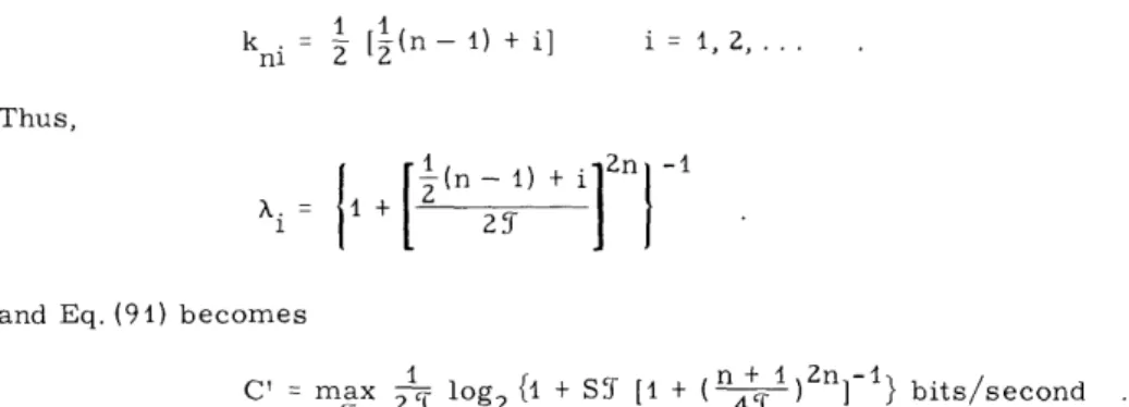
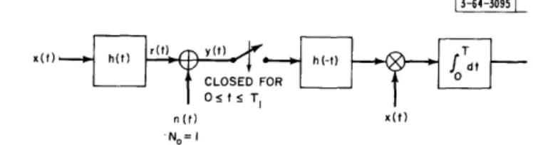
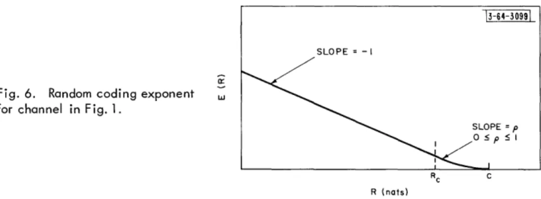
In Sec. I-E, it was demonstrated that a useful model for digital communication over fixed time-continuous channels with memory considers the transmission of signals of T-seconds dura-tion through the channel of Fig. 1 and the observadura-tion of the received signal y(t) for T1 seconds. Given this model, the problem is to determine the probability of error for an optimum detector and a particular set of signals and then to minimize the probability of error over the available sets of signals. Under the assumption that the vector space representation is appropriate for this situation, there remains the problem of selecting the basis functions for both the transmitted signals x(t) and the received signals y(t).

13-64-30941

x(t)

n(t)

manx

y(t)

Fig. 1. Time-continuous channel with memory.

f n(t)

[I H(f) 12/N(f ]

f

If x, n, and y are the (column) vector representations of the transmitted signal (assumed to be defined on O, T), additive noise, and received signal (over the observation interval of T

seconds), respectively, an arbitrary choice of basis functions will lead to the vector equation

y = [H] x + n (7)

in which all vectors are, in general, infinite dimensional, n may have correlated components, and [H] will be an infinite dimensional matrix related to the filter impulse response and the sets

of basis functions selected.t If, instead, both sets of basis functions are selected in the manner presented here and elsewhere, it will be found (1) that [H] is a diagonal matrix whose entries are the square root of the eigenvalues of a related integral equation, and (2) that the components of n are statistically independent and identically distributed Gaussian random variables. Because of these two properties it is possible to obtain a meaningful and relatively simple bound on prob-ability of error for the channel considered in this work.

In the following discussion it would be possible, at least in principle, to present a single procedure for obtaining the desired basis functions which would be valid for any filter impulse response, any noise spectral density, and any observation interval, finite or infinite. This approach, however, leads to a number of mathematically involved limiting arguments when white noise and/or an infinite observation interval is of interest. Because of these difficulties

the following situations are considered separately and in the order indicated.

tit is, of course, possible to obtain statistically independent noise components by using for the receiver signal

space basis functions the orthonormal functions used in the Karhunen-Loeve expansion of the noise5 4,6 0 How-ever, this will not, in general, diagonalize [H].

12

Arbitrary filter, white noise, arbitrary observation interval (arbitrary T1); Arbitrary filter, colored noise, infinite observation interval (T1 = ); Arbitrary filter, colored noise, finite observation interval (T₁ < o).

Due to their mathematical nature, the main results of this section are presented in the form of several theorems. First, however, some assumptions and simplifying notation will be

introduced.

Assumptions.

(1) The time functions h(t), x(t), y(t), and n(t) are in all cases real. (2) The input signal x(t) may be nonzero only on the interval [0, T] and has

finite energy; that is, x(t) E 2(0, T) and thus

T j (t)dt x2 :

x(t)

dt x(t) dt <

~.i0it

(3) The filter impulse response h(t) is physically realizable and stable.5 6 Thus, h(t) = 0 for t < 0 and

5

_oo

(4) The time scale for y(t) is shifted to remove any pure delay in h(t). (5) The observation interval for y(t) is the interval [0, T1], unless otherwise

indicated.

Note: Assumptions 3, 4, and 5 have been made primarily to simplify the proof that the p (t) are complete. Clearly, these assumptions cause no loss of generality with respect to "real world" communication problems. Furthermore, completeness proofs, although considerably more tedious, are possible only under the assumption that

'

_oo

Notation.

The standard inner product on the interval [0, T] is written (f, g); that is, T

(f, g) 4x f(t) g(t) dt

The linear integral operation on f(t, s) by k(t, T) is written kf(t, s); that is,

kf(t, s) A k(t, T) f(T, s) dT

The generalized inner product on the interval [0, T1] is written (f, kg)_T

that is, 1

(f, kg)T __i f(t) kg(t) dt f (t) k(t, ) g(T) d dt

(f. kg 1 O:T1 ,,,,Soo

With these preliminaries the pertinent theorems can now be stated. The following results are closely related to the spectral decomposition of linear self-adjoint operators on a Hilbert

13

space.62,63,66 It should be mentioned that all the following results can be applied directly to time-discrete channels by simply replacing integral operators with matrix operators.

1. Basis Functions for White Noise and an Arbitrary Observation Interval

Theorem 1.

Let N(f) = 1, define a symmetric function K(t, s) = sponse by

K(t, s) {oT h(T - t) h(T - S) dT

K(s, t) in terms of the filter impulse

re-0 t, s _ T

elsewhere and define a set of eigenfunctions and eigenvalues by

Xi i(t) = K i(t)_{11 1}

i = 1,2,... . (8)

[Here and throughout the remainder of this work, it is assumed that i(t) = 0 for t < 0 and t > T, i = 1, 2, .... Then the vector representation of an arbitrary x(t) E 2(0, T) is x, where

Xi = (x, Si) and the vector representation of the correspondingt y(t) on the interval [0, T₁]

(T1 > T)t is given by Eq. (7) in which the components of n are statistically independent and iden-tically distributed Gaussian random variables with zero-mean and unit variance and

[H]

X1

I,

2

Ff n 0

The basis functions for y(t) are {Oi(t)}, where

1 h(tp (t)

ei(t)= Aii i

TO

t Telsewhere

elsewhere and the it h component of y is

Yi = ( y ' i)T

64,65

Note: To be consistent with the literature, ' it is necessary to denote as eigenfunctions only those solutions of Eq. (8) having Xi > 0. This restriction is required since mathematicians normally place the eigenvalue on the right-hand side of Eq. (8) and do not consider eigenfunctions with infinite eigenvalue.

t The representation for y(t) neglects a noise "remainder term" which is irrelevant in the present work. See the discussion following the proof of Lemma 3 for a detailed consideration of this point.

tAIl the following statements will be true if T1 < T except that the i(t)} will not be complete in 2(0,T).

Proof.

The proof of this theorem consists of a series of Lemmas. The first Lemma demonstrates that eigenfunctions of Eq. (8) form a basis for z2(0, T), i.e., that they are complete.

Lemma l(a).

If T > T, the set of functions {i(t)} defined by Eq. (8) form an orthonormal basis for f?2(0, T), that is, for every x(t) E 2(0, T)

x(t) = L xii(t) 0 t < T i=l

where x = (x, i) and mean-square convergence is obtained. Proof.

Since the kernel of Eq. (8) is 2 (see Appendix A) and symmetric, it is well known6 4 that at least one eigenfunction of Eq. (8) is nonzero, that all nonzero and nondegenerate eigenfunctions are orthogonal (and therefore may be assumed orthonormal) and that degenerate eigenfunctions are linearly independent and of finite multiplicity and may be orthonormalized. Furthermore, it is known6 1'6 5 that the {(Pi(t)} are complete in 2(0, T) if and only if the condition

(f, Kf)T 0 f(t) E 2(0,T)

1

implies f(t) = O almost everywhere on [0, T]. But (f Kf)T₁ s

[

Thus, to prove completeness, it suffices to prove that if T

f f(r) h(t - ) d = 0 0 t T1 with T1 >_T then f(t) = 0 almost everywhere on [O, T]. Let

u(t) =T f(T) h(t - ) dt and assume that

O tt< T

u(t) =

z(t-T 1) t > T1

where z(t) is zero for t < 0 and is arbitrary elsewhere, except that it must be the result of passing some 2(0, T) signal through h(t). Then

0

1

U(s) u(t) e- s t dt = e Z(s) = F(s) H(s) Re[s] > 0 (9)

Now, for Re[s] > 0,

15

-[Z(s)

I=

So

'

~~)

However, from the Schwarz inequality,

I f(T) dT [<

0

L o

If(T) dT I h(t) dt

_00

and, from assumption 3,

\ h(t) l dt < o Joo

Thus,

IZ(s) <

[T

Since f(t) E

z2(0,

IF(s) H(s) < A exp{I-Re[s] T1}

From a Lemma of Titchmarsh it follows a + = T1, such that

IF(s) | < AI exp{-Re[s] a}

JH(s) I < AZ exp {-Re[s] 1f}

where A1A2 = A. Finally, since

f(t) =

27rj

~_'

j-|I h(t) dt < 0 Re[s] > 0

Eq. (9) implies that there exists a constant A

for Re[s] 0

that there exist constants a and f with

Re[s] 0

Re[s] > 0

F(s) est ds

and similarly

h(t) 27rj

5

these conditions and ordinary contour integration around a right half-plane contour imply that f(t) = 0

h(t) = 0

t <a

t<

From assumptions 3 and 4, h(t) is physically realizable and contains no pure delay. Thus, by choosing = 0, it follows that a = T1and, if T1> T, that f(t) = 0 almost everywhere on [0, T]. This completes the proof that the {POi(t)} are complete.

16 dt drT < 0

1/ZJ

J

d

The following Lemma demonstrates that the {0i(t)} defined in the statement of the theorem are a basis for all signals at the filter output, i.e., all signals of the form

ST r(t) = X(T) h(t - T) dT 0 0.< t < T x(t) 22(0, T) Lemma l(b).

Let r(t) and Oi(t) be as defined previously. Then c0

0. t T1 r(t) = , riO i(t)

i=

where r_i = (r, i)T = xi, xi = (x, i), and uniform convergence 9 is obtained.

Proof.

Define two functions rn(t) and xn(t) by n xn(t) A i=l XiP i(t) 0< t T where x. ₁ (x, i )₁ and T( 0 0 t T1 Then Jr(t) - rn(t) I ST [x(T) - Xn(r)] h(t -T IX(T) - Xn

(r)

I

Thus, from the Schwarz inequality,

I r(t) - r(t) I T 0 sT₀ However, by assumption oo h2 (t) dt < o 17 r) dr X(T) - Xn (T) dT h (t - ) dr 0 x(r ) 2 dTr h

(t)

~~~~-0

___I

___·_

I

_

^_____

and Lemma l(a) proved that lim , I X(T) (T) n-oo Thus, lim Ir (t) - rn(t) = 0 n-oo

and uniform convergence is obtained. Since

n n rn (t) = xiOihq(t) x xe (t) i= i= 1 it follows that o0 r(t) = , ixi i (t ) i=l

and therefore that

(r, ej) T = / i j i T1 But (Oj0 i)T -1 i "NTi )T t

~~

Z,

and the Lemma is proved.

The following Lemma presents the pertinent facts relating to the representation of n(t) by the functions {Oi(t)}.

Lemma l(c).

Let the {i(t)} be as defined above. Then the additive Gaussian noise n(t) can be written as

n(t) = niOi(t) + nr(t) i= o. t T1 where ni = (n, i)T 1 n. = 0 1 n.n= 6.. 1 J 1J 18 0< t T1₁ Thus, __. __ 1_ _ I_

oo

and the random processes niOi(t) and nr(t) are statistically independent. i=l

Proof.t

Defining

nr (t) = n(t) -

,

i=l

it follows that n(t) can process. Therefore,

be represented in the form indicated. By assumption, n(t) is a zero-mean

ni = (n, Oi)_{1 T1 T} = (n, ei)T = _T t

and

nin. _ij (n, i)T _iT, i(n,)T _{)T )Tj}= t n(T) n(t) Oi(7) ej(t) dTdt

1

1

0

T₁ T1 6(, - t) ei(T) ej(t) ddt = ( Oj)T i

(Note that unit variance is obtained here due to the normalization assumed in Fig. .) Next, let ns(t) be defined as

x0

0 t < T₁ ns(t) M= niei(t)

i= 1 and define n and nr by_-s

ns = [ns(t), 2,ns (tn)]

nr =[nr(t ),nr(t 2).. nr(t)]

Then, the random processes ns(t) and nr(t) will be statistically independent if and only if the joint density function for ns and n factors into a product of the individual density functions, that is, if

P(ns,nr) = P1(ns) P2(nr) for all {ti} and {ti}

t

o0

n.(t) does not converge and since n(t) is infinite bandwidth white noise for which time samples do not exist.

i=1

However, this argument is of interest for several reasons: (a) it leads to a heuristically satisfying result, (b) the same result has been obtained by Price70 in a more rigorous but considerably more involved derivation, and (c) it can be applied without apology to the colored noise problems considered later.

However, since all processes are Gaussian it can be readily shown that this factoring occurs when all terms in the joint covariance matrix of the form n (ti ) nr(ti) vanish. From the previous definitions

ns(t) nr(t') =

[ ni0i(t)]

[n(t')-

E

nioi(t']

i

0i(T) ei(t) d- E

Z

i j

= , 0i(t') Ei(t)- E i(t) ei(t) =0

i i

Combining the results of these three Lemmas, it follows that for any x(t) E S2 (0, T)

x(t) = , xi~qi(t) i and y(t) = Yiei(t) + nr(t) i where Xi = (x, i) and Yi =yi ( y' i i) T

~T1

F

Thus, only the presence of the noise "remainder term" nr(t) prevents the direct use of the vector equation

y = [H] x+ n

It will be found in all of the succeeding analyses, however, that the statistical independence of the ns(t) and nr(t) processes would cause nr(t) to have no effect on probability of error. Thus, for the present work, nr(t) can be deleted from the received signal space without loss of gener-ality. This leads to the desired vector space representation presented in the statement of the

theorem. Q.E.D.

2. Basis Functions for Colored Noise and Infinite Observation Interval

This section specifies basis functions for colored noise and a doubly infinite observation in-terval. Since many portions of the proof of the following theorem are similar to the proof of Theorem 1, reference will be made to the previous work where possible. For physical, as well

as mathematical, reasons the analysis of this section assumes that the following condition is satisfied:

o N(f) df < o

Theorem 2.

Let the noise of Fig. 1 have a spectral density N(f), define two symmetric functions K(t - s) and K1 (t - s) by

K(t- s) N(f) exp [jc0(t - s)] df 0< t, s T

0 elsewhere

and

K(t - s) N(f)- exp[jc(t - s) dt

and define a set of eigenfunctions and eigenvalues by

Xi °i (t ) K(p (t)

i i = i i 1, , ... (10)

Then the vector representation of an arbitrary x(t) E 2(0, T) is x, where x = (x, Sqi) and the vector representation of the corresponding y(t) on the doubly infinite interval [-oo, o] is given by Eq. (7) in which [H] and n have the same properties as in Theorem 1. The basis functions for y(t) are

h i (t) Ot <

ei(t) =

~

and the it h component of y is

Yi = <y, Ki>` y(t) Kei(t) dt Proof.

Under the conditions assumed for this theorem, the functions {i(t)} of Eq. (10) are simply a special case of Eq. (8) with T = +o. Thus, they form a basis for 22(0, T) and the representa-tion for x(t) follows directly. [See Lemma l(a) for a proof of this result and a discussion of the convergence obtained.] By defining Oi(t) as it was previously defined, it follows directly from Lemma (b) that the filter output r(t) is given by

tBecause N(f) is an arbitrary spectral density, it is possible that N(f)- 1will be unbounded for large f and there-fore that the integral defining K1(t - s) will not exist in a strict sense. It will be observed, however, that

Kl(t -s) is always used under an integral sign in such a manner that the over-all operation is physically

mean-ingful. It should be noted that the detection of a known signal in the presence of colored Gaussian noise involves an identical operation.5 4

21

r(t) X. x.O(t) i= I Furthermore, since <oi K0j> = 1 _{<h i, K hqpj>} P i(u) h(t - a) _{|d [ K} 1(t - s) j(p) h(s - p) dp ds dt T T (P i()

sj4p)

(

ei(~) (0 jP) N(f) exp [jw(o- p)] df d dp

((P_i Kji)T = X . x . i, j) ij 1 it follows that <r, K10i> = i xi and thus that

<r, K1Oi> Oi(t) i=l

Finally, with I n(7) and ni defined by

R

()

N(f) eWT

=5

f

5

5

5in(t

-_ -co

Foo

Fo

S°°

r

T

_.

Y4

1

1

_

II

or

nn = -o Oi(a) ej(p) Kl1( - p) dodp = <Oi, K >= 6ij

From this it is readily shown, following a procedure identical to that used in Lemma (c), that the random processes ns(t) and nr(t) defined by

ns(t) n i i(t) izl

nr(t) _ n(t) - ns(t)

are statistically independent. Thus, neglecting the "remainder term" leads to

y(t) = yiei(t) i 1 where

Yi = <Y Kii> = AXi x + ni or, in vector notation,

y = [H x + n

3. Basis Functions for Colored Noise and Finite Observation Interval

This section specifies basis functions for colored noise and an arbitrary, finite observation interval. As in Sec. II-D-Z, it is assumed that

o N(f) -df <c

Ni(f)I2

Theorem 3.

Let the noise of Fig. 1 have a spectral density N(f), define a functiont K1(t, s) by

(t - ) K1(u, s) do = 6 (t - s) 0,< t, s T where ~(T ) _i N(f) ej C₇ df define a function K(t, s) by K(t, s) s i {a h(u - t) K(O, p) h(p - s) d dp O t, s T

0 Cme hfon ieia t hsi er l pl elsewhere

t Comments identical to those in the footnote to Theorem 2 also apply to this "function."

23

and define a set of eigenfunctions and eigenvalues by

Xi Fi(t) = K i(t)_{11 1}

i

Then the vector representation of an arbitrary x(t) e Y2(0, T) is x, where x.i = (x, eoi) and the

-- 1 i

vector representation of the corresponding y(t) on the interval [0, T1] is given by Eq. (7) in which [H] and n have the same properties as in Theorem 1. The basis functions for y(t) are

h(p t) ei(t)= ₀ Xi

and the it h component of y is

Yi = (y, KI1i)T

0 t T1

elsewhere

Proof.

This proof consists of a series of Lemmas. erty of a complete set of orthonormal functions.

The first Lemma presents an interesting

prop-Lemma 3(a).

Let {Yi(t)} be an arbitrary set of orthonormal functions that form a basis for S ₂(0, T1), i.e.,

they are complete in 22(0, T1). Then

00

Z

i=i

in the sense that for any f(t) e 2(0, T1 )

l.i.M. •o_{n-- 0}

0 <t, s T1

| Yi(t₎ i(r) du = f(t)

i-i

Proof.

By definition, a set of orthonormal functions {yi(t)} that are complete in S2(0, T₁) have the property that for any f(t) 22(0, T1)

n

f(t) = l.i.m. E (f, Yi)T Yi(t)

n-oo i1 1

T f(t) = L.i.m. f(a)

n--oo

o

The following Lemma provides a constructive proof that the function K1(t, s) defined in the theorem exists. 24 that is, t T1 [ i(a ) Yi(t) da i=

Lemma 3(b).

Define a function Kn(t - s) by

Kn(t--

0 < t, s T1

elsewhere

and define a set of eigenfunctions {Yi(t)} and eigenvalues {ii} by

fiYi(t) = KnYi(t) s) Kl(t, s₎ = , i( t ) i ( s ) 0o t T₁ i= 1,2,.. O0 t, s < T i=l Proof.

From Mercer's theorem it is known that

L PiTi(t) yi (s) i pi :_ A i 0O t, s T 0 < t, s T1 it follows that

- ) K1(a, s) d = _{yj(t) Yi(s) (j,Yi)T}

iT

= Yi(t) i(s) i

This result, together with Lemma 3(a) and the known61 fact that the {yi(t)} are complete, finishes the proof.

Lemma 3(c).

If T1 > T, the {pi(t)} defined by Eq.(11) form an orthonormal basis for s2(0, T), that is, for every x(t) E 2(0, T) 00 x(t)= i= 1 xiq i(t) 0 t T where

x = (x, ° i) and convergence is mean square. i 25 Then Thus, with in (t - s) Kt(t, s) I T n(t

0:

fl

..

fl

1 3

Proof.

Since K(t, s) is an S2-kernel,t it follows from the proof of Lemma l(a) that the {oi(t)} are complete in S 2(0, T) if and only if the condition

(f, Kf)T = 0

implies f(t) 0= almost everywhere on [0, T]. But

(f, Kf)T $$= 1 f(t) h(a - t) Kl(c, p) h(p -s) f(s) dt ds d dp

Thus, from Lemma 3(b),

(f',KF)T= i [Ki f(t) h(a - t) i(cr) dt da i

and it follows that the condition (f, Kf)T = 0

implies

Si

IfST

However, the completeness of the yi(t) implies that the only function orthogonal to all the yi(t) is the function that is zero almost everywhere.65 Thus (f, Kf)T 0 implies

T

f(t) h(a - t) dt = 0 almost everywhere on [0, T₁]

and, from the proof of Lemma (a), it follows that, for T₁ > T, f(t)= 0 almost everywhere on [0,T]. This finishes the proof that the {p0 i(t)} are complete. The following paragraph outlines a proof of the remainder of the theorem.

With i(t) as previously defined, it follows directly from Lemmas (b) and 3(c) that for any x(t) E 2(0, T) the filter output r(t) is given by

so

r(t)= L ixiei (t ) t T

i=l

Furthermore, by a procedure identical to that in Theorem 2, it follows that

_ (T Kj)T 6ij

which implies that

(r, KO)T i x i

t See Appendix A.