Dynamic systems and subadditive functionals

Dynamic Systems and Subadditive Functionals

by

Sleiman M. Itani

Submitted to the Department of Electrical Engineering and Computer

Science

in partial fulfillment of the requirements for the degree of

Doctor of Philosophy in Electrical Engineering and Computer Science

at the

MASSACHUSETTS INSTITUTE OF TECHNOLOGY

June 2009

@

Massachusetts Institute of Technology 2009. All rights reserved.

ARCHIVES

Author ...

Departme ttof Electrical Engineering and Computer Science

May 1, 2009

Certified by...

Munther A. Dahleh

Professor

Tbesis Supervisor

Certified by ...

I -iliio Frazzoli

Professor

Thesis Supervisor

Accepted by ...

Terry P. Orlando

Chairman, Department Committee on Graduate Students

MASSACHUSETTS INSTTUTE OF TECHNOLOGY

AUG 072009 1

Dynamic Systems and Subadditive Functionals

by

Sleiman M. Itani

Submitted to the Department of Electrical Engineering and Computer Science

on May 1, 2009, in partial fulfillment of the

requirements for the degree of

Doctor of Philosophy in Electrical Engineering and Computer Science

Abstract

Consider a problem where a number of dynamic systems are required to travel between

points in minimum time. The study of this problem is traditionally divided into two

parts: A combinatorial part that assigns points to every dynamic system and assigns

the order of the traversal of the points, and a path planning part that produces the

appropriate control for the dynamic systems to allow them to travel between the

points. The first part of the problem is usually studied without consideration for

the dynamic constraints of the systems, and this is usually compensated for in the

second part. Ignoring the dynamics of the system in the combinatorial part of the

problem can significantly compromise performance. In this work, we introduce a

framework that allows us to tackle both of these parts at the same time. To that

order, we introduce a class of functionals we call the Quasi-Euclidean functionals, and

use them to study such problems for dynamic systems. We determine the asymptotic

behavior of the costs of these problems, when the points are randomly distributed

and their number tends to infinity. We show the applicability of our framework

by producing results for the Traveling Salesperson Problem (TSP) and Minimum

Bipartite Matching Problem (MBMP) for dynamic systems.

Thesis Supervisor: Munther A. Dahleh

Title: Professor

Thesis Supervisor: Emilio Frazzoli

Title: Professor

Acknowledgments

First and Foremost, I thank God for everything good I ever had. I thank God for

putting God, faith and a whole lot of wonderful people in my life.

After that, I would like to thank my mother Sawsan Barbir for being everything

she is, the example of distilled love, selflessness, and care in the world. If I have to

dedicate anything to anybody, it would definitely be dedicated to you. I've seen what

you have gone through for me and my siblings, and I know that I can never repay

you; so I just want you to know that I appreciate everything. If it weren't for your

love of knowledge and your encouragement, I would have never went into science.

I would really like to thank Professor Munther A. Dahleh, my advisor. You were

always the bearer of good news to me, you put up with my procrastination and you

were always there when I needed you. You are, with no competition, the best advisor

ever. I know that I was the luckiest graduate student ever. I hope someday I'll be

like you.

My co-advisor, professor Emilio Frazzoli, I thank you for sharing your deep insight,

offering your great advice, and giving your great support. Your being there made the

PhD journey much smoother and nicer. I will always appreciate that. Professor

Alexander Megretski, my committee member, I thank you for all of your insight,

help, and encouragement. Your impact on my thesis was extremely substantial.

For all of the people who touched my life and left an everlasting impression in

my character, I would like to convey my deepest and most sincere appreciation. My

dearest sister Douha and brothers Mustapha and Ibrahim, I just love you all so much

and thank you for more things than I can think of. My close friends who know me so

well they look into my soul, Taha, Abdelkader, Saif, Yahya and all of the guys from

school, you were always great brothers, perfect friends and wonderful people and for

that I would like to thank you. Mr. Saud Kawwas and Mr. Abdelraheem Hajjar,

I would like to thank you for all the things you taught me about life, dreams and

myself.

Iyad, Nabil, Antonio, Hani, Naamani, Spiro, Wissam, Roy, Karaki, Layal, Joelle,

Manar, Tarifi, Rani, and Rawia, a great group with great memories. You guys are

just amazing.

My friends from MIT, just having you guys around makes everything much better.

Even MIT wasn't so bad because you guys were here, so Costas, Sree, Yola, Hanan,

Demba, Erin, Aykut, Mesrob, Pari, Amir Ali, Paul, Ermin, Mitra, Mardivic, Georgos,

Keith, Holly, Micheal and all my friends from LIDS: I would like to thank you all for

being great friends through these four years. My dear friend and collaborator Karen,

your friendship and help over the years has definitely changed my life. You're a really

great friend, and I am really thankful that I went to that Grad Rat.

Contents

1 Introduction 13

1.1 Motivation ... .... . ... ... 13

1.2 Previous Work . .. . . . .. ... 14

2 Problem formulation and Background 17 2.1 Problem Formulation . . .. .. . .... ... 17

2.1.1 Problems with Subadditive Cost for Dynamic Systems . . .. 18

2.2 Dynamic System Models that are Affine in Control . ... 22

2.2.1 Examples of Dynamic Systems of Interest . ... . .. 23

2.3 Dynamic Systems Background .... ... ... 26

2.3.1 Evolution of the Output under Inputs from the family Ap(u, t) 32 2.3.2 Chen-Fliess Series for Nonlinear Control Systems . ... 36

2.4 Subadditive Euclidean Functionals . ... ... 37

3 Local Behavior of Dynamic Systems 43 3.1 Elementary Output Vector Fields of a Dynamic System ... 44

3.1.1 Examples . ... ... 46

3.1.2 LTI systems ... ... 47

3.2 Bounds on the Area of the Reachable Set ... .. .... ... 51

3.2.1 Upper Bound on the Volume of the Small-Time Reachable Set 51 3.2.2 Lower Bound on the Volume of the Reachable Set ... . 52

3.3 Locally Steering Dynamic Systems ... 58

4 Quasi-Euclidean Functionals

4.1 Notation for Quasi-Euclidean Functionals . 4.2 Quasi-Euclidean Functionals' Properties . 4.3 Quasi-Euclidean Functionals' Results . . . .

4.3.1 Variables with General Distributions 4.3.2 Requirements Relaxations . ... 4.4 Quasi-Euclidean Functionals Applications .

5 Quasi-Euclidean Functionals and Small-Time Controllable Dynamic Systems

5.1 Local and Global Behavior of Monotone, Subadditive Functionals 5.2 Applications to Problems with Locally Controllable Dynamic Systems 5.3 TSP Algorithm for Small-Time Controllable Dynamic Systems . .

5.3.1 Algorithm Description ... 5.3.2 Time to Trace the Tour ...

6 Problems for Dynamic Systems with Drift

6.1 Dynamic Systems with Drift ... 6.2 DyTSP Upper bound . ...

6.2.1 Level Algorithm . ... 6.2.2 Time to trace CLA ...

6.3 Heterogenous Dynamic systems ...

6.3.1 Piece-wise Uniform Dynamic Systems . . . .

6.3.2 Local Transformations for dynamic systems

7 Dynamic Traveling Repairperson Problem for Dynamic Systems

7.1 Problem Formulation ... 7.2 Low Traffic Intensity ...

7.3 High Traffic Intensity ...

8 Conclusion 8.1 Conclusions ... 63 . . . . 6 3 .. . . . . 64 .. . . . 66 . .. . . . . . . 6 7 .. . . . 69 .. . . . . . 71 83 ... . . . 8 3 .. . . 86 ... . . . . 8 6 .... 89 .. . . . 92 .. . . . . 92 . . . . . 93 97 97 98 100 105 105

A Appendix

A.1 Proofs for Dynamic Systems . . . ..

A.1.1 Proof of theorem 2.2 . . . ..

A.2 Proofs for the TSP for Dynamic Systems

A.2.1 Proof of lemma 6.16 . . . ..

A.3 Proofs for Quasi-Euclidean Functionals .

A.3.1 Proof of theorem 4.7 . . . .

A.3.2 Proof of lemma 4.7 . . . ..

A.3.3 Proof of lemma 4.8 . . . ..

A.3.4 Proof of theorem 4.8 . . . ..

A.3.5 Proof of lemma 4.10 . . . ..

A.3.6 Proof of lemma 5.11 and 6.18 . .

A.3.7 Proof of lemma 5.13 . . . ..

107 107 107 109 109 111 111 116 117 118 120 122 123 - I I I I

List of Figures

2-1 Parameters for a car pulling k-trailers ...

.. . .

23

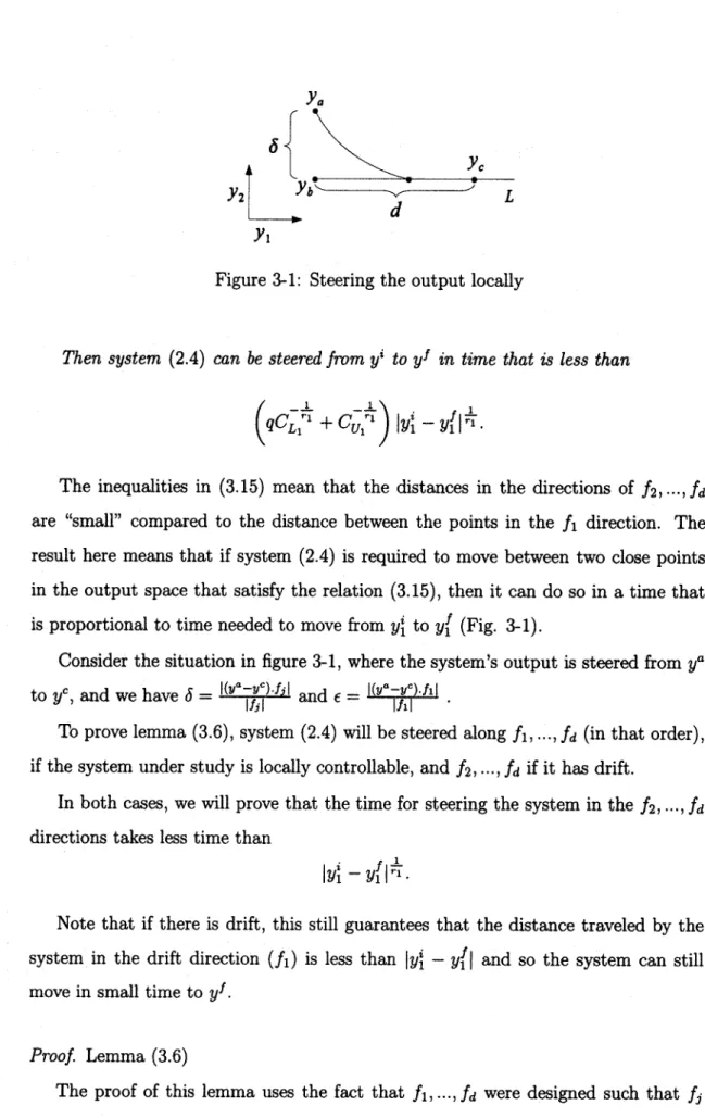
3-1 Steering the output locally ....

.

...

59

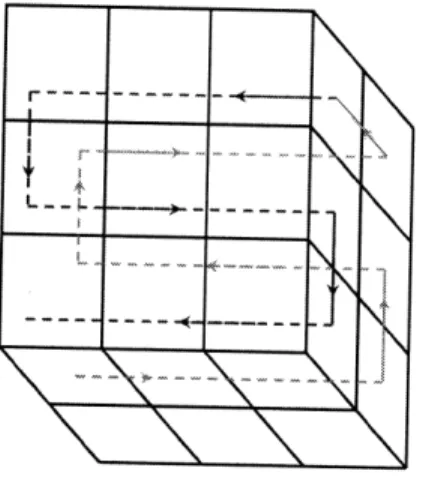
5-1 A tour visiting all of the cuboids in the partition. . ...

..

80

Chapter 1

Introduction

In this thesis, we study combinatorial problems under dynamic constraints, that is, combinatorial problems where the cost depends on the evolution of the output of a dynamic system. We aim to create a framework that allows the study of the asymp-totic behavior of a class of such problems for dynamic systems. We also seek to show the applicability of the framework by producing results on some interesting combi-natorial problems for dynamic systems. We start here by motivating the problem we study.

1.1

Motivation

The main motivation for the problems we study are applications where a given set of dynamic systems are required to travel as quickly as possible between a set of points. One example of such applications is a surveillance mission where a given UAV equipped with sensors has to visit a number of checkpoints as quickly as possible. Another one is the vehicle-target matching problem, where a team of n UAV's are spread over a bounded area, and there are n targets that are also randomly distributed in the same area. Each target must be visited by a UAV while minimizing the average time it takes for the targets to be visited. The dynamic system and the targets in such problems are usually modeled as point masses. Such problems have been studied by first solving a combinatorial problem that concentrates on assigning points to each

dynamic system and/or determining the order of traversal of the points while ignoring the dynamic constraints on the system [60, 61, 62]. An optimal control problem aiming at making the dynamic systems follow the solution of the combinatorial problem in the minimum time is then solved. In general, solving the combinatorial part of the problem while ignoring the dynamics of the system can lead to bad performance. In [14], the authors study the TSP for a dynamic system that moves with a constant velocity and has bounded curvature (the Dubins Vehicle). They prove that getting the optimal order for the Euclidean TSP and using it for the TSP for the Dubins vehicle produces (in certain situations) an error that grows at least as a constant times the number of points. Such deterioration in performance makes it important to include the dynamics of the system in the combinatorial part of the problem, and is the main motivation for our work.

Problems similar to the ones introduced above are becoming more interesting with the increase of our use of UAV's and autonomous robots for different kinds of applications. These problems range from vehicles traveling for pickup or delivery, to surveillance and search-and-rescue missions [60, 61, 12, 55]. Although certain aspects of these problems have been studied before, we tackle these problems while accounting for the dynamics of the system(s) that are required to perform the mission and traverse the resulting path. We study how the dynamics of the robot or the UAV affect the asymptotic behavior of the cost of the problem. This gives a more accurate understanding of the problem and insight on how to minimize the associated cost, and provides fundamental limits on performance. Additionally, we provide algorithms that produce order optimal paths that the dynamic systems can trace, and thus they can be used for the applications for UAV's and robots.

1.2

Previous Work

Because of the importance of studying combinatorial problems under dynamic con-straints, some interesting combinatorial problems have been recently studied for spe-cific dynamic systems. The Traveling Salesperson Problem has been recently studied

for the Dubins vehicle [1, 28], the double integrator [4], the Reeds-Shepp car, the

dif-ferential drive robot [22]. Additionally, in our previous work [6, 7, 8], we studied the

TSP and some related problems for a general dynamic system having a state space

representation that is affine in control. Our work is a natural extension of that work

to a larger class of problems for dynamic systems.

This work is a generalization of some previous work in a different sense. In this

work, we introduce a framework for studying general combinatorial problems where

dynamic systems travel through a given set of points. Using this framework, we

concentrate on studying the behavior of the cost of the problem as the number of

points tends to infinity. This is inspired by the similar study of the costs of the

Euclidean versions of such combinatorial problems [1, 2]. This direction of studying

such problems has proven effective in many ways, producing important convergence

results for the stochastic versions of the problems and bounds on the worst-case

results [11]. Additionally, this way of studying the costs can be used to produce

approximation algorithms for the combinatorial problems. We therefore use the same

approach in our work here and direct our efforts at studying the asymptotic properties

of the costs of the problems when the points are randomly distributed and their

number tends to infinity. Thus the problem we deal with here can be considered a

generalization of the one studied in [1, 2] to account for the dynamic constraints of

the system.

The rest of this Thesis is organized as follows: Chapter 2 has the problem

formula-tion and introduces some background on dynamic systems and subadditive Euclidean

functionals. In Chapter 3 contains a study of the local behavior of dynamic systems

and establish results on the time needed for a dynamic system to move locally

be-tween two points. In Chapter 4, Subadditive Quasi-Euclidean functionals are defined

and their properties are studied, these will be of utmost importance for our results.

Chapter 5 studies the relationship between problems for small-time locally

control-lable dynamic systems and Quasi-Euclidean functionals and determines the

asymp-totic behavior of the costs of those problems. The applicability of the formalism with

some specific examples of problems for dynamic systems and their corresponding costs

under dynamic constraints. Chapter 6 relaxes the initial assumptions on the dynamic systems, and produce an algorithm for the TSP for a general dynamic system. Chap-ter 7 has a detailed study of the Dynamic Traveling Repairperson Problem, with algorithms that perform within a constant factor of the optimal for low intensity and high intensity cases. Chapter 8 has the conclusions and discussion.

Chapter 2

Problem formulation and

Background

In this chapter, we formulate the problem of interest and present some important background from the literature. The background needed can be divided into two parts: The first is about dynamic systems and their local behavior, and the second is about subadditive Euclidean functionals. These two parts represent the two areas that we are merging in this work. Since we are injecting dynamics into traditionally combinatorial problems, it is essential that we build some background in both of those areas. We start by introducing the models of the dynamic systems that we use in our study.

2.1

Problem Formulation

The goal of this work is to produce a framework that allows the study of combinatorial problems under dynamic constraints, that is, combinatorial problems where the cost depends on the evolution of a controlled dynamic system. The framework should allow us to study a class of interesting problems under dynamic constraints.

2.1.1

_{Problems with Subadditive Cost for Dynamic Systems}

Since our aim is to incorporate dynamic constraints to classical combinatorial prob-lems, we start by reviewing the classical formulation of the combinatorial problems that we generalize in this work. These are combinatorial problems on a, given graph. A graph is defined by its nodes and edges. Thus a graph G is defined as (y, E), where y = {yl,..., y}, y C Rd is a set of points and E = {(i,j)ti,j e {1,...,n}} is a

set of ordered pairs each of which corresponds to a directed edge of G. This means that (io, jo)

E

in the graph. The combinatorial problems we study choose a subset of the edges of the given graph. To denote the chosen edges, an n x n binary matrix Z is used, where n _{is the number of vertices in the graph. Thus the variables that we use for} the optimization are zij, _{and the classical versions of the problems can be formulated} as follows:

L() = in w(yi, j)zij, (2.1)

i j

where T C {0, 1}nx" _{is a set that enforces a certain structure on Z. We study}

a generalization of the previous problems where the weights are produced from a dynamic system. Consider an example where a dynamic system (UAV or a car) is required to travel between a number of points in minimum time. In this example, the cost of an edge connecting two points y' and y doesn't only depend on yi and y5, but it also depends on the state of the dynamic system at yi and yj. Thus we consider that the points in = {yi, ... , y,} are in the output space of m dynamic systems whose states we denote by x and whose output equation is y = h(x). Without loss of generality, we assume that n > m and that yl,..., y,, are the output points corresponding to the initial states Xi, ..., x, of the dynamic systems (yi = h(i), for

Ls(x

... x, Y) = minm

ZET xi:h(xi)=yi,i=m+1,...,n _(2.2)

i,3

(2.2)

y - h(xi), Vi = 1, ..., m,

where Ts is a function that depends on the evolution of the dynamic system. Thus the minimization is over the states that correspond to points in y other than the initial

states. In particular, we are interested in the case where Ts(xi, xj) is the minimum time needed for a the state of a dynamic system to move from xi to xj with bounded input: Ts(x,

xj)

90()+

gi(X)

x(0)

=

z(T) = xj.

In this equation, the dynamic system is modeled with a state space representation that is affine in control. We describe systems that are affine in control and study some of their properties later in this section. Different costs Ts(xi, xj) might be studied in a similar fashion,

The weights in the combinatorial problem are the minimum time needed for the dynamic system to move its output between pairs of points in y. Of course, this time depends on the state of the system and not only on its output. Thus when the dynamics are inserted into the problem, both minimization over the control in (2.3) and over the state in (2.2) are needed.

What we study here is the asymptotic behavior of the costs (Ls : Rd-+ R) of such problems when the points are sampled from a random variable 74 and their number tends to infinity. This is a generalization of the study for the classical Euclidean case (where the cost w(yi, yj) is the Euclidean distance between y and yj) that was done by Beardwood, Halton and Hammersley [2] and later generalized by Steele [1]. Thus our study can be considered to be a generalization of their results to account for the

dynamics of the system traversing the paths. We aim to introduce a, framework for the study of such problems, and determine some sufficient properties of Ls that allow us to directly determine the asymptotic behavior of Ls as n - oc. We will start by studying these problems when the dynamic system has no drift (go = 0) and Y, ... , Y, are uniformly, independently and identically distributed in [0, 1]", and then extend the results to non-uniform distributions and systems with drift.

Two functionals that we will use to show the applicability of our framework are the costs of the Dynamic System Traveling Salesperson Problem and the Dynamic System Minimum Bipartite Matching Problem. These are special cases of the functionals described in equations (2.2) and (2.3) that are given by:

1. DyTSP: (Dynamic system TSP) Find the minimum cost Hamiltonian circuit over

Y

L (x1, y)

-

ZTs(xi,xy)z.j,

> 2

VV c y, 2 <

Vl

< n - 1.

The requirement on Z means that there should be one incoming edge and one outgoing edge for every node in the graph, and that the graph should be connected.

points in y while minimizing the average (or total) travel time:

Ll(x,...,

x, y)

=

min

min

Ts(Xi, xj)z,j,

h(xk) = Yk,

k

= n

+

1,...,2n

Ezi,

1,

zijO

ViE {1,...,n},

J a

Z y=O,

Zi

=1

ViE{n+l-1,...,2n}.

a J

The requirement here on Z means that V i,j

j

{1, ...,

n},

there should be an

outgoing edge from each yj and an incoming edge into each y?.

In both of these problems, Ts(xi, xj) is the minimum time needed for a dynamic

system to move its state from xi to

xj

as in (2.3). We study these examples as

important applications of our results on the general class of problems. We study the

properties they satisfy and their asymptotic behavior when

yl,...

,

y,

are randomly,

We also seek algorithms for the DyTSP as a practical application of the framework.

Finally, we study the DTRP (Dynamic Traveling Repairperson Problem) for dynamic

systems.

DTRP for Dynamic Systems

Given a dynamic system that is modeled as in (2.4), let R be compact region in

the output space of the system (R is assumed to be a d-dimensional cuboid with

dimensions W

, W

,...,

Wq).

We study the DTRP, where "customer service requests"

are arising according to a Poisson process with rate A and, once a request arrives, it

is randomly assigned a position in R uniformly and independently.

The repairperson is modeled as in (2.4) and is required to visit the customers and

service their requests. At each customer's location, the repairperson spends a service

time s which is a random variable with finite mean 3 and second moment s2. We

study the expected waiting time a customer has to wait between the request arrival

time and the time of service, and we mainly focus on how that quantity scales in terms

of the traffic intensity A- for low traffic (AT -+ 0) and high traffic (AX -- 1). We also

study the stability of the queuing system, namely whether the necessary condition

for stability (A < 1) is also sufficient.

2.2

_{Dynamic System Models that are Affine in}

Control

In the problem formulation, the costs Ts(xi, xj) are functions of the evolution of a

dynamic system. We model the dynamic systems with state space models that are

affine in control,have an output in Rd and bounded input. Thus they are described

as follows:

go(x) +

gi(x) Ui,

(2.4)

i=1

y

h(x).

x(0) = z0,

U = {u(.) : measurable R -- [- M, M]}.

We will use Assumption 3.3 in most of this work, and then in Chapter 6 generalize

the results for the cases where the dynamic system has drift. This class of systems

is very general and descriptive. We use this class of models for the dynamic systems

because even though it is general, studying its local behavior properties using

differ-ential geometric methods is mathematically elegant and established in the literature

[25, 26]. The boundedness on the input is assumed because unbounded inputs can

make minimum time problems trivial.

(Y1Yz2) (x x )

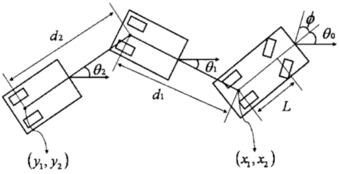
Figure 2-1: Parameters for a car pulling k-trailers

We use these examples throughout this thesis to clarify certain concepts about local reachability of dynamic systems and the behavior of the TSP and similar problems for dynamic systems.

2.2.1

Examples of Dynamic Systems of Interest

The first model we use is that of a linear time-invariant system with its output in R3 The state space model of that system is as follows:

i = Ax + Bu

(2.5)

and

l

, ui (-) : R

-+

[-1, 1].

Here, go, gi, 92 are given by:

go = Ax -X2

3x

0

0

1

0

0

The second example is a simplified model of a car pulling k trailers (from [31]).

The first two states in that model are the location of the first car in the plane and the rest are the angles at the axles of the trailers; the output is the location of the last trailer (Fig. 2-1). The state space model for the car is therefore [31]:

= cos(0o)

L

=

_{sin(9o -}

₀₁₎

if

Oj)

j=1 (2.10)

k-1

Ok = cos(Oj- C -

8Oj)

X1 _ kC=1

di

S - Ek=1 di sin(Oi)

u

= {f(.) = tan((.)), (.) R: R - [-o, 0o]}.

The car is assumed to have a constant speed forward, and the control we have on the car is the steering angle q (actually tan(O)). It is easy to see that this is a special

case of our general dynamic system (2.4), where go and gl are given by:

cos(Oo)

sin(Oo)

(

i

cos(O_

-

I)) sin(8i-

- Bi)

SHj= cos(O- 1 - Oj) sin(Ok-1 8Ok)

0 0 1 L g1 = 0 0

We will follow these systems throughout this work to clarify some concepts. Ad-ditionally, in our detailed study of the TSP and DTRP for dynamic systems, we will generate the asymptotic solutions of the TSP/DTRP for these examples to demon-strate our results for some specific dynamic systems.

2.3

Dynamic Systems Background

We first introduce some terminology and definitions for systems that are affine in control; most of these definitions are standard in the literature [25, 26]. We will in general use subscripts to indicate components of a, vector, and superscripts to label individual instances. Thus xi will indicate the

ith

We start by introducing the most basic object we need, the reachable set of a dynamic system.

Definition 2.1 (Reachable set). Given T > 0, the reachable set from state xz for a

dynamic system is the set RT(xo) of states x such that V x1 E RT, 3 ut, u2, ..., u* E U such that:

x(0)

=

x

, x(T)

=

z,

This is the set of states that are reachable in exactly time T. We define the set of states reachable in time less than or equal to T by:

R<T(xo) = Uo<t<TRt(xo).

We extend the previous definition to the output space, and so we define the output-reachable set from a state xz to be the set OT(xo) of points

y

=

and

O<T(x ) = Uo<t<Ot(x 0).

We indicate by A<T(x) the volume of O<T(xz).

We turn to some important properties of some systems that are affine in control.

Definition 2.2 (Small-time Locally Controllable Systems). A system is small-time

locally controllable at zx E R

if 3 T > 0 such that

x

E Interior(R<t(xo)) V t such that 0 < t < T.

We call a system small-time locally controllable if it is small-time locally controllable

at all x E RP.

is output small-time locally controllable at x0 _{if 3 T > 0 such that}

h(xo) E Interior(O<t(xo)) V t such that 0 < t < T.

Definition 2.3 (Output small-time locally controllable systems). A system is called

"output small-time locally controllable" if it is output small-time locally controllable for every x in R.

Definition 2.4 (Vector Fields). For all the purposes of this work, a vector field f(x)

is a smooth mapping from RP to RP.

Given a vector field

f

along

f

by:

L(f (x), wt(x)) _Oxifi(W

i=1

Note that

£(f(x),x i (x)) = fj (x).

Given a vector field f and g : RP -- R, we call the derivative of g along f the new

RP -R q function:

L (f(x), g(x)) - O(x) f(x)

where 9 is the Jacobian matrix of g.

Note that the ith component of £(f, g) is the derivative of the function gi along

f.

Definition 2.5 (Lie Brackets). Given two vector fields f and g, the Lie bracket (or product) of f and g is another vector field denoted by [f, g] and is given by:

gg Of

[f ,

g]()

=

f

g(x),

Lie brackets can be iterated since the result of a Lie bracket is itself a vector field.

A notion that is related to the iteration of vector fields of a dynamic system that is

affine in control is the "order" of a Lie bracket.

Definition 2.6 (Order of Lie Brackets). The orders of Lie brackets of a dynamic

system as in (2.4) are defined iteratively as follows:

1. The order of gi, i E {, ..., m} is defined to be 1.

2. The order of [gi, gJ] is the sum of the order of gi and the order of gj, where gi and gj are themselves in go, ... , gm or iterated Lie brackets of go,..., g,.

Definition 2.7 (Indices of an iterated Lie Bracket). Given vector fields gl, ...,gm,

note that an iterated Lie bracket V of gl, ..., g, that has order r is determined by the

following:

1. An ordered set of indices , Iv = (il; ...; i,), ik E {1,..., m}, that determine the

vector fields from {gi, ..., g m that are in V, and their order in V. This set of indices is defined iteratively as follows:

I9 = i is {1, ...m},

I[91,g2] = gg' U Ig2,

with the order conserved.

2. An ordered set By = ((il; jl); ...; (ir-l, -)) of r- I pairs designating the order in which the iterated Lie brackets are applied. This set of indices is also defined iteratively:

Bg = iE {1, ..., m},

B[gi,g2] =

Bg1

the addition Bg2 + rgl is defined as follows: -~ z f r, l - -- i f B , 2 - 5 {B2 + T91}

if B

S{(i

Definition 2.8 ({Ap(u

t)}). We introduce a family of inputs, denoted by {Ap(ui, t)},

that is related to gl, ..., g, and their Lie brackets. We use the notation Ap(ui, t) (apply ui for time t), which is defined as follows:

1. Ap(ui, t) means to set the input ui = 1 and uj = 0, j fi for a time duration equal to t. Ap(-ui, t) means to set the input ui = -1 and uj = 0,j fi for a time duration equal to t.

2. Ap([u , u], t) = Ap(ui, t) o Ap(uj, t) o Ap(-ui, t) o Ap(-uj, t), where o denotes concatenation and u and uj might be brackets themselves.

Definition 2.9 (Order of Ap(u', t)). The "order" of an input Ap(ui, t) is defined

similarly to the order of Lie brackets of the dynamic system:

1. The order of Ap(uj, t), i E {1, ..., m} is defined to be 1.

2. The order of Ap([ui, uJ], t) is the sum of the order of Ap(u , t) and the order of

Ap(u , t).

We introduce the notation for the "projection" of state space Lie brackets onto the output space.

Definition 2.10 (Domain Space Lie Brackets). Given analytic vector fields fi, ... ,

fs

_fl,

_fs

in the domain space of k as follows:

[fil]k=

(fi,

E

[f1, f2]k = 1(f1, [.f2]k) -

£(f

.

where fi and

,g} or are lie brackets of gi,

Note that the operator

[]k takes vector fields in RP to vector fields in Rd. Thus [fl]k = C(fl,k), [fl, f2]k =

£ (fi, £(f2, k)) - £(f 2,

L(fi,

The order and indices of domain space Lie brackets are defined similarly to those

of Lie Brackets in Definitions 2.6-2.7.

To denote a generic Lie Bracket of gl, ... , gm, we will use the notation [gi]. To

denote an output space Lie bracket of gi, ... , gm we will use the notation [gi]h and to denote a generic input in the family

{Ap(ui,

Definition 2.11 (Nilpotent Systems). A dynamic system that is affine in control is called nilpotent if the Lie brackets of {go, gl, ... , gm} vanish after a certain order. This happens for example when the vector fields are polynomials.

Some additional notions that we use in our study for both the local behavior of dynamic systems and Quasi-Euclidean functionals are the following:

Definition 2.12 (Dilation function (k') ). Given an ordered set of positive real numbers r = (rl,., rd, ), define the function k' : R -- Rd componentwise, by setting

kz(aV) = ai . Note that the ordering in r affects k'.

Definition 2.13 (Asymptotic Notation). Finally, we use the standard asymptotic

notation for the scaling of functions, and thus we say a function f(n) is O(g(n)) if

3c, N > 0 such that f(n) < cg(n) V n > N.

We say f(n) is Q(g(n)) if g(n) is O(f(n)). f(n) is E(g(n)) if f(n) is O(g(n)) and

Q(g(n)). Finally, f(1) is o(g(l)) if limio f(l) = 0 (for functions) or limn (oonf = 0

2.3.1

_{Evolution of the Output under Inputs from the family}

Ap(u

, t)

We start with the following theorem about the evolution of the output of dynamic systems when inputs from the family {Ap(u , t)} are applied. First note that the time needed to apply the input Ap([u~], t) is equal to a[%]t, where a[i] is a constant that only depends on the indices of u'.

Theorem 2.1. Consider the dynamic system given in (2.4). If the input Ap([u], t)

(whose order is r) is applied, then

y(c

.it)

G (gi,

i=0 k

where [gi]hlxo is the output space Lie bracket with the same indices as [u], that is,

I l[O = Uui]

and

xo

B

B=

gm,

is

to gl,..., g, whose order is higher than r and is evaluated at x0_.

Proof. The proof is by mathematical induction. If the input Ap(ui, t) is applied, then by theorem 2.2, the state and output of the dynamic system evolve as:

0Ctk

x(t) = Xo+ E Ik(gj X)_ k=l

y(t) = y(0) + E 'k(gi, h(xo))

k=l

If the input Ap([ui uj], t) = Ap(u', t) o Ap(uj, t) o Ap(-ui, t) o Ap(-uj, t) is applied, then the state and output of the dynamic system evolve as:

x (t) = X0 + (gi, .rO))

k=l

=1

y(t)

y(0) +

>

!

x2 = x(2t) = o0 (g, (x)) k=l k=l = 0 _{k i(gX (X0))t} O k (g (0 tk k=l k=l 0c L( tki +k2 + 1 k _{(gj 2(g x O))) t}

_k!k2

=y(O) + L (g h(x°)) - + I2(g, h(xO))k + E

:

) )) !kt k=1 k=1 kl=l k2=1 (2.14) 00 tk 0 0 tk 0 0 (

(t)k

~

x(3t)

=o

x())

= X0 C2k(gi X(XO))- 0 k 0 - E k(g k2 gix 2O)))

k=l k=l kl=l k2=l1 + (i ( ))) (-1)kltkl+k2 k (g k ( 1(g 0 ))) klt+k2 k_l=l k₂=1 kl=l k2=1 (k1)l ktkl3+k2+k3

k!k2!k3!

+EEE

)

+

,

h(x))

-+

))

NL

(g

Lk2h()

+ L? k(gi, L2(gih(x)))(t +

j

ki k2!

y(4t) = y(O) + E (gi k 1 t

y(4t) = y(O)+ (g, h(xo))+ + E k(gi,

h(xl))-k=l k=l

+

(s,

a(x

)) i( k h(k 3)

k=1 k=l1

= (o) + E 22t2 iC _- 02 2t2k k kh tkkgL

(xO))(2k)! E C2k(gj h(xO)) ' + E E Ck,(gJ fk2(gih(xO))) ki_.

k=1 k=1 _{ki=l k} 2 1! + 0

>

1:

Lk3(g))

>

3

"Y kk=2kk>k(+k+k kl(gJFL2(gji 3(g, h(xO)))) ( -)kl k2

3 1k!k2!k3! kz=I k2=1 k3=1 + £k(gJ _{kg i L 0gi,~} 4(g h()))))l)+k )k+k2:k23(

_kl!k2!k3!

After collecting the coefficients of t2_:

y(4t) = y(O) + t2 (C2(gi, h(x0)) + C2(g, h(x°)) -

C(gi,

£(gj,

>

i=O k

OO

= y(O) + t2 [gi, gjh zo + t3 ti F k(gij, h (xo0)), i=0 k

(2.18)

higher than 2 and is evaluated at x

_{. Similarly,}

OO

x(4t) =

x(o)),

i=O k

where F (gi, gj) is a derivative of x with respect to gi and gy whose order is higher

than 2 and is evaluated at x.

Given an input Ap([ui], t), let r(ui) be the order of u

_.

_{Assume that if r(u') E}

{1,

...

, s - 1} and the input Ap([ui],

t)

is applied, then

01.

y(c[]it) = y(O) + t'r(') [gihjxO + tr(u)+l ti E Fk 91, ..., m

h

,

i=0 k

where [gi]h is the output Lie bracket that has the same indices as [ui], and

Fk (gl, .. ,

h(x

)) is a derivative of h with respect to gl, ..., gm whose order is

higher than r(u2) and is evaluated at xz

2.

x(O[ui]t) -= X(0) + tr(u') i +zo tr(u +1 ik (gl, **, i()),

i=O k

where [g'] is the Lie bracket that has the same indices as [ui], and F(g., ..

, x(x))

is a derivative of x with respect to gl,

...,

gi whose order is higher than r(ui)

and is evaluated at x.

We aim to prove that if Ap([ui], t) is applied, where r([ui])

=

s, then

y(ai]t) = y(O) + tS[gi]h + t"s t' Fi(gl, ...,

gm, h(x),

i=O k

where [g]h is the output Lie bracket that has the same indices as

[u'],

and Fk(gl, .., g, h(xO))

is a derivative of h with respect to gY,

...,

g whose order is higher than s and is

eval-uated at x

.

This can be done by using the above assumption and the fact that given [ui] such

that r([u'])

=

s, then [u'] = [u, u'] , where r([u']) < s and r([u]) < s and using the

We now turn to an important series representation for dynamic systems. One side of the importance of this representation is that it gives a lot of insight about the local behavior of the dynamic system. We therefore use it in Chapter 3 to study the scaling of the area of the small-time reachable set of the system in terms of time.

2.3.2

Chen-Fliess Series for Nonlinear Control Systems

The formal power series property of the Chen-Fliess series allows a representation of the evolution of nonlinear control systems that are described as in (2.4). This representation is given by the following theorem:

Theorem 2.2. [25]

If go, ... , gm, h are analytic functions, then 3T > 0 such that Vt < T, the jfh component of the output of system (2.4) evolves as follows:

yj(t) = hj(xo) (2.19)

S(gi

o,

h(x

)))

dik

...

<o,

k=0 io=0 ik=0

Where the integral in (2.19) is defined iteratively by:

o (t) = t,

j

(t)=

_{j (7)d7,}

J

k

...

io

=

i

k

(-)

T

d

ik

...

o.

An important consequence of this theorem is a set of necessary and sufficient conditions for an output yj not to be affected by an input ui [25]. Specifically, yj is unaffected by ui if

£(gi, h) = 0

S(g

i,

(gi, ...

I

(gYi hj(xo)))) = 0,

This result hints at the usefulness of the Chen-Fliess series in small-time optimal control problems, and is indirectly used in our study of the small-time behavior of dynamic systems in Chapter 3. The proof of the theorem is in [25] and is repeated in the appendix for easy reference. We finally note that this theorem directly implies that

xj (t) =

Xj(xo)

(2.20)

+

EE

..

_{E (gio,}

_.0,

₀

₎₎

_JO

_i

k=O io=0 ik=0O

This equation describes the evolution of the state of a dynamic system in small-time as a series. The integrals in the end can be used to describe the small-time scaling effect of each set of Lie derivatives. When using constant inputs, a single integral scales like t, a double integral scales as t2_{. Therefore it hints that lower order Lie}

derivatives dominate in the small-time setting.

We now turn to some background on the other side of the problems we are ad-dressing, namely the cost of the combinatorial problem. The background here deals with the costs in the case where the distance between every two points is the Eu-clidean distance between them. We modify this work later to allow the use of an approximation of the time a dynamic system needs to move between points in its output space.

2.4

Subadditive Euclidean Functionals

In the case where the weights of the edges in the our problem formulation in Sec-tion 2.1 are given by the Euclidean distances between the points, the costs of the TSP is known to belong to a class of functionals called subadditive Quasi-Euclidean functionals [1]. Additionally, it can be shown that the cost of the Euclidean version of MBMP is also similar to subadditive Euclidean functionals when d > 3 [12]. We therefore turn to introduce subadditive Euclidean functionals, study their properties

and produce some of the known results on them. Subadditive Euclidean Functionals were introduced by Steele in [1], and are defined as follows:

Denote by L a real valued function of the finite subsets of Rd (d > 2). Lis a Euclidean functional if it satisfies the two following properties[]:

Property 1 (Homogeneity). L({cal,...,oax,}) = aL({xl,...,, }) Va E R+,x E Rd.

Property 2 (Translation Invariance). L({xi + x,..., x, + x}) = L({zx, ... , x,}) Vx

Rd

A functional L is called bounded, monotone and subadditive if is satisfies the fol-lowing three properties:

Property 3 (Boundedness). Var(L({Xi, ..., X,})) < oc if the Xi's are independently and uniformly distributed in [0, 1]'.

Property 4 (Monotonicity). L(x U A) > L(A) Vx

E

Let

Qj,

are parallel to the axis and have length 1 and let tQj = {xjx = ty, yE

Q}.

Property 5. (Subadditivity)

IC ER such that Vm E N and tE R+ xi j... xn E R ,

L({xi, ... , x,} n [0, t]d) < E L({xl, ... , x,} n tQi) + Ctmd - (2.21)

i=1

Subadditive Euclidean functionals have been studied in [1]. The first result pro-duced in that work and is relevant to our work here is the following theorem:

Theorem 2.3. If L is a functional that satisfies properties 1-5, and Xi; 1 < i < 00

are independent and uniformly distributed in [0, 1]d, then there exists a constant 3(L) such that:

li L({XI, ...

X,})

lim 1 = (L) a.s.

OO 7~ 1- d

This theorem signifies that a monotone subadditive Euclidean functional is

asymp-totically sub-linear in the number of variables, or, more interestingly, that it behaves

as /(L)n1d when n is large. This result was used to prove that the length of the

Euclidean TSP, the cost of Euclidean minimum spanning tree and the cost of the

Euclidean minimum matching problem all scale as n'-.

Some additional properties can be used to generalize the previous theorem to the

case where the variables are not uniformly distributed. These properties are simple

subadditivity, scale boundedness, and upper linearity.

A functional L is simply subadditive if it satisfies the following property:

Property 6 (Simple Subadditivity). 3B such that:

L(A1 U A2)

<

for all finite subsets A1 and A2 of [0, t]d, V t > 0.

It is is called scale bounded if it satisfies the following property:

Property 7 (Scale Boundedness). 1B such that:

, n < _{B, Vn > 1, t > 1,}

(2.24)

tn 1

and

{x,...,

Finally, a functional L is upper linear if it satisfies the following property:

Property 8 (Upper Linearity). For any finite collection of cubes

Qi,

1 < i

<

s

(Qi

defined above), and any infinite sequence xi, 1 < i

<

oc, in Rd

L satisfies:

S

E L({xi,...,xn,}

n

Q)

<

L({xl,...,xn}

n

u=lQi) + o(n1-).

(2.25)

i=1

Using these properties allows the following theorem to hold:

Theorem 2.4. If L is a functional that satisfies properties 1-8, and {X} are i.i.d.

their distribution is f(x), then B3(L) such that:

L(XI...'X})

f

lim ( (L) f(x)l dx a.s. (2.26)

n---oo ₁ d

An interesting part of this theorem is that )(L) is the same from the uniform

distribution case, the only difference between the the asymptotic behavior of L under

different distributions of X 1, ... ,X, is the factor fpd f(x)'-dx. This means that

/(L)

can be calculated from the case of the uniform distribution (for example), and

then the asymptotic behavior of L can be determined under any distribution f(x) of

Now that we have introduced all of the background we need from the literature

to tackle the problems at hand, we start by dealing with the time a dynamic system

needs to move its output between two points in its output space. We will mainly

focus on the case where the two points are close to each other, in the sense that the

system can travel between them in a small amount of time. We also introduce the

notion of the r-warped distance between two points. The idea of r-warped distance

is very central to bringing dynamic constraints to combinatorial problems.

Once we have studied the small-time behavior of dynamic systems, we can deal

with the first two of our main problems. Namely, we study the TSP and DTRP for

dynamic systems in detail. We produce lower bounds on the costs of the problems

and algorithms that scale optimally.

Next, we introduce and study a class of functionals that we call subadditive

Quasi-Euclidean functionals. The properties of these functionals are inspired by the

small-time properties of the minimum small-time curves of dynamic systems. We introduce their

properties, and produce results paralleling the results we have here for subadditive

Euclidean functionals. We also show that if the weights in the graphs (as described

in Section 2.1.1) are the r-warped distances between the points, then all of the costs

of interest are subadditive Quasi-Euclidean functionals. This allows us to determine

the asymptotic behavior of the costs of problems of interest when the weights are

the r-warped distances. Since the notion of the r-warped distance was inspired by

the local behavior of dynamic systems, these results bring us one step closer to the

desired results on combinatorial problems for dynamic systems.

Finally, we use subadditive Quasi-Euclidean functionals to generalize the results

for the TSP and DTRP of dynamic systems to a larger class of problems. We link

problems for dynamic systems with the problems for the r-warped distance and deduce

results about the asymptotic behavior of the costs of the given combinatorial problems

under dynamic constraints.

Chapter 3

Local Behavior of Dynamic

Systems

In this chapter, we study the local behavior of dynamic systems. As we will see later in this work, the local behavior of the system governs the global results in the problems that we are interested in. This is mainly because of the subadditivity property of the functionals we deal with, as we will see later in chapter 5. We will specifically study the distance a given dynamic system S can move its output in a certain direction f when it is given a small time t. Of course, the scaling (in terms of t) of the volume of the small-time reachable set will follow. For most of the thesis, we have the following assumptions on the dynamic system in (2.4):

Assumption 3.1. h, go, g9, ... , gm are analytic functions.

Assumption 3.2. The integral curves of go,, l, m, gm are defined.

Assumption 3.3. The system is small-time locally controllable, so without loss of

generality, go=0.

This chapter is divided into four sections: In the first section, we introduce some entities that are very important for our study of the small-time reachability prop-erties of dynamic systems. These are the elementary output vector fields and their corresponding orders. In the second section, we bound how the area of the output-reachable set OT(zo) (definition 2.1) of system (2.4) scales in terms of T as T -- 0.

In the third section, we study how to steer system (2.4) between two points that are close together. This provides a bound on performance, and makes our results more applicable. In the final section we introduce the notion of the r-warped distance between points. We relate the idea of the r-warped distance between points in the output space of a dynamic system to the time the dynamic systems needs to move its output between those points. This notion will be very useful to us when we insert dynamics into the combinatorial problems of interest, as we will see in chapters 4 and

5.

3.1

Elementary Output Vector Fields of a Dynamic

System

Given an initial state

x

at yO = h(xo) as follows:

Definition 3.14 (Elementary Output Vector Fields). Let ri(xo) be the smallest

natural number such that there are rl vector fields in the set {gi, ..., g,, (denoted

g , ... gr -) that satisfy:

(g , ..., C (gl , h(zO))) . (3.1)

Assumption 3.4. There exists a non-zero iterated Lie bracket in the output space,

designated pj1(xo), such that the order of pl(xo) is equal to rl.

For

j

I

(9g -.. g1, h(xo))) (3.2)

being linearly independent of p(x

), ...

-

1(xo).

Assumption 3.5. If

-(go,* .(g 7 _j-,(xO))o ) span{ l, ... '' j- } ,