Dynamics of multi-body space interferometers including reaction wheel gyroscopic stiffening effects : structurally connected and electromagnetic formation of flying architectures

Structurally Connected and Electromagnetic Formation Flying Architectures by

Laila Mireille Elias MASSACHUS

OF TEC B.S., Aeronautics and Astronautics

_JUL

University of Washington, 1998

S.M., Aeronautics and Astronautics

LIBR

SUBMITTED TO THE DEPARTMENT OF AERONAUTICS AND ASTRONAUTICS IN PARTIAL FULFILLMENT OF THE DEGREE OF

DOCTORATE OF PHILOSOPHY IN AERONAUTICS AND ASTRONAUTICS at the

MASSACHUSETTS INSTITUTE OF TECHNOLOGY June 2004 ETTS INSTTVTE HNOLOGY 1

2004

ARIES

AERO

@ 2004 Massachusetts Institute of Technology. All rights reserved.

Signature of Author ...

Certified by ...

Certified by ...

Department of Aeronautics and Astronautics March 12, 2004

Associate Professor David W. Miller Thesj4 Committee Chairman

Dr. Raymond Sedwick J4esis Committee Member

Certified by . . . ... ..1 .- . . . . . Dr. Marthinus Van Schoor Thesis Committee Member

Accepted by . . . .

Edward M. Greitzer H.N. Slater Professor of Aeronautics and Astronautics Chair, Committee on Graduate Students

Structurally Connected and Electromagnetic Formation Flying Architectures by

LAILA MIREILLE ELIAS

Submitted to the Department of Aeronautics and Astronautics on March 12, 2004 in Partial Fulfillment of the

Requirements for the Degree of Doctorate of Philosophy at the Massachusetts Institute of Technology

ABSTRACT

Space telescopes have the potential to revolutionize astronomy and our search for life-supporting planets beyond our Solar System. Free of atmospheric distortions, they are able to provide a much "clearer" view of the universe than ground-based telescopes. A developing technology that appears promising is space-based interferometry, which uses multiple apertures separated at great distances to act as a large virtual aperture. In this way, interferometers will achieve angular resolutions far greater than those achievable by monolithic telescopes. In this thesis, we investigate the dynamics and control of two pro-posed architectures for spaceborne interferometers: structurally connected interferometers and electromagnetic formation flying interferometers.

For structurally connected interferometers, we develop a coupled disturbance analysis method that accurately predicts a space telescope's optical performance in the presence of reaction wheel v ibrational disturbances. T his method "couples" a reaction wheel to a structure using estimates of the accelerances (or mobilities) of both bodies. This coupled analysis method is validated on the Micro-Precision Interferometer testbed at NASA's Jet Propulsion Laboratory. The predictions show great improvement over a simplified "decoupled" analysis method when compared to experimental data.

For formation flying interferometers, we consider the use of electromagnets as relative position actuators. A high fidelity, nonlinear dynamic model of a deep-space electromag-netic formation flight (EMFF) array is derived from first principles. The nonlinear dynamics are linearized for a two-vehicle array about a nominal trajectory, and the linear-ized model is shown to be unstable, but controllable, and therefore stabilizable. A linear optimal controller is designed for the system and implemented to form the closed-loop dynamics. Time simulations of the closed-loop nonlinear dynamics demonstrate that EMFF using linear control proves very effective, despite the nonlinearities of the system's dynamics and the electromagnetic actuators.

Thesis Supervisor: David W. Miller

Associate Professor of Aeronautics and Astronautics

This work was performed partially under contract with NASA's Jet Propulsion Laboratory at t he C alifornia I nstitute o f Technology, p artially under c ontract NRO-000-02-C03 87-CLIN0001 with the National Reconnaissance Office and Lt. Col. John Comtois as techni-cal scientific officer, and partially under contract 07600-097 with the NASA Institute for Advanced Concepts and Dr. Robert A. Cassanova as technical monitor. The author grate-fully thanks the sponsors for their generous support that enabled this research. The author also thanks Zonta International for the honor and the emotional and financial support offered by the Amelia Earhart Fellowship.

The author also wishes to thank Professor David Miller for supporting this research, for inspiring new ideas, and for having enough faith in his students to allow them to perform independent research. Dr. Ray Sedwick and Dr. Marthinus Van Schoor both offered valu-able advice and feedback and greatly influenced this work. Their willingness to spend time discussing the work and to make thought-provoking suggestions inspired a great deal of this research.

The departmental readers of this thesis, Professor Jonathan How and Professor Charles Coleman, spent a great deal of their personal time critiquing this thesis, and that effort is greatly appreciated.

Ipek Basdogan, Lisa Sievers, and Frank Dekens were wonderful to work with at JPL and taught me a great deal. I look forward to rejoining their team.

SharonLeah Brown deserves special thanks not only for her incredible job as fiscal officer, but also for b eing a friend and big sister t o me. Her support and c oncern c arried me through the preparation of this thesis, even when the task seemed impossible. Marilyn Good was also there, not only to help with scheduling meetings and travel arrangements, but to offer a smiling face and a gentle manner when they were most lacking.

The technical and personal support from my friends and colleagues in the lab has been amazing, and I w ant t o t hank Sam S chweighart, D an K won, Edmund K ong, Matthew Neave, Alvar Saenz-Otero, Scott Uebelhart, Rebecca Masterson, Jeremy Yung, Tim Glenn (for this thesis template!), and everyone else who helped shape my experience at MIT. I learned an immense amount from each of you and have been truly humbled by your abili-ties. Thank you for inspiring me.

My family and their support have been without parallel. There is no way to express my appreciation to my parents, Ziad and Ralda, my sister and brother, Maria and Paul, and my second family, Phil, Barb, Nat, Theresa, and Andrew for the amazing and unfailing sup-port they have given me. They remind me that, despite being surrounded my amazing people, I, too, can accomplish this task if I keep trying. I could not have done so without their support.

Finally, my husband, David Cutler, has been my backbone throughout the last six years at MIT. His unconditional faith in me both surprises me and drives me to accomplish my goals. His love and support are superhuman, and for that I thank him.

A bstract . . . . iii Acknowledgments . . . . Table of Contents . . . . . List of Figures . . . . List of Tables . . . . . . . . . . . . V Vii xi . . . . xv

Nom enclature . . . . xvii

Chapter 1. Introduction . . . 1

1.1 Motivation . . . 1

1.2 Research Objectives and Approach . . . 3

1.2.1 Structurally Connected Interferometer . . . 4

1.2.2 Formation Flying Interferometer . . . 6

1.3 Literature Review . . . 8

1.3.1 Review of Flexible Body Coupling Literature . . . 8

1.3.2 Review of Formation Flight Literature . . . 9

1.4 Thesis Overview . . . . 11

Chapter 2. Structural Dynamic Coupling Theory . . . . 2.1 Introduction . . . . 2.2 Decoupled Disturbance Analysis Method . . . . 2.3 Coupled Disturbance Analysis Method . . . . 2.3.1 Motivation for Coupled Analysis Method . . . 2.3.2 The Load Filter . . . . 2.3.3 Coupled Analysis Method . . . . 2.4 Summary and Conclusions . . . . Chapter 3. Structural Dynamic Coupling Experiments . 3.1 M PI Testbed . . . . 3.1.1 MPI Testbed Description . . . . 3.1.2 MPI Testbed Transfer Functions . . . .

13 13 14 16 16 17 20 23 25 26 26 26 Vii

TABLE OF CONTENTS

3.2 Intermediate Results . . . . 3.2.1 Hardmounted Reaction Wheel Disturbance Spectra . . . . 3.2.2 On-MPI Reaction Wheel Disturbance Spectra . . . . 3.2.3 MPI Accelerances . . . . 3.2.4 Reaction Wheel Accelerances . . . . 3.2.5 Performance Measurements . . . .

3.3 Performance Predictions . . . . 3.3.1 Decoupled Analysis . . . . 3.3.2 Coupled Analysis Using "rigid-RW, model3-MPI" Filters . . . 3.3.3 Coupled Analysis Using "rigid-RW, model6-MPI" Filters . . . 3.3.4 Coupled Analysis Using "rigid-gyro-RW, model6-MPI" Filters 3.3.5 Decoupled Analysis Using Cross-Spectral Density Terms . . . 3.4 Summary and Conclusions . . . . Chapter 4. Review of Kane's Method . . . . 4.1 Introduction . . . . 4.2 D efinitions . . . .

4.2.1 Generalized Coordinates and Configuration Constraints 4.2.2 Generalized Speeds and Motion Constraints (Holonomic

nomic Systems) . . . . 4.2.3 Partial Velocities and Partial Angular Velocities . . . . 4.2.4 Generalized Active Forces . . . . 4.2.5 Generalized Inertia Forces . . . . 4.3

4.4 4.5 4.6

vs.

Nonholo-Kane's Equations of Motion . . . . Example Using Kane's Equations . . . . Applicability of Kane's Equations to EMFF Systems Summary and Conclusions . . . . Chapter 5. Electromagnetic Formation Flight Dynamics

5.1 Introduction . . . . 5.2 System Description . . . . 5.2.1 Vehicle Description . . . . 5.2.2 Coordinate Frames . . . . 5.2.3 Degrees of Freedom . . . . 5.2.4 Rotation Matrices . . . . 5.2.5 Velocity Vectors . . . . 5.2.6 Actuator Description . . . . . . . . 73 . . . . 73 . . . . 74 . . . . 75 . . . . 76 . . . . 78 . . . . 80 . . . . 81 . . . . 88 28 28 30 30 32 40 41 41 42 43 45 49 50 53 53 54 54 54 56 57 60 64 65 69 70 viii

5.3.1 Magnetic Moment Vectors Expressed in Global Coordinates

5.3.2 Calculation of Electromagnetic Forces and Torques . . . .

92 93

5.4 Nonlinear Equations of Motion . . . . 95

5.4.1 Generalized Coordinates and Generalized Speeds . . . . 96

5.4.2 Partial Velocities and Partial Angular Velocities . . . . 97

5.4.3 Generalized Forces . . . . 99

5.4.4 Nonlinear Equations of Motion . . . 113

5.4.5 Nonlinear Equations of Motion with Infinite Spring Stiffness . . . . 118

5.5 Summary and Conclusions . . . 120

Chapter 6. Electromagnetic Formation Flight Dynamics Analysis . . . 123

6.1 System Description . . . 124

6.2 Linearized Equations of Motion . . . 134

6.2.1 Nominal Trajectory . . . 134

6.2.2 Nominal Control . . . 137

6.2.3 Conservation of Angular Momentum . . . 141

6.2.4 Linearization of Equations . . . 142

6.3 Stability Analysis of Linearized Dynamics . . . 151

6.3.1 System Eigenvalues . . . 151

6.3.2 System Mode Shapes . . . 154

6.4 Controllability Analysis of Linearized Dynamics . . . 155

6.4.1 Full Degree-of-Freedom, Full Actuator System . . . 155

6.4.2 Full Degree-of-Freedom, Reduced Actuator System . . . 156

6.4.3 Reduced Degree-of-Freedom, Reduced Actuator System . . . 158

6.5 Optimal Control Design Using Linearized Dynamics . . . 159

6.6 Summary and Conclusions . . . 162

Chapter 7. Electromagnetic Formation Flight Control Simulations . . . 165

7.1 Introduction . . . 165

7.2 Dynamics Simulation Method . . . 165

7.2.1 Simulation Tools . . . 165

7.2.2 Simulation Approach . . . 166

7.3 Simulation Results . . . 167

7.4 Summary and Conclusions . . . 170

TABLE OF CONTENTS

8.1 Thesis Summary . . . . 8.2 Thesis Contributions . . . . 8.3 Recommendations for Future Work . . . . 8.4 Concluding Remarks . . . . R eferences . . . .

Appendix A. Empirical Force Filters . . . .

Appendix B. Two-Vehicle EMFF Symbolic Eigenvalues

Appendix C. Two-Vehicle EMFF Optimal Gains . . . . Appendix D. EMFF Control Experiments . . . . D. 1 Linear Airtrack . . . .

D. 1.1 Airtrack Description ...

D. 1.2 Airtrack Dynamics and Control . . . . D. 1.3 Discussion of System Poles . . . . D. 1.4 Airtrack Experimental Results . . . . D.2 Planar Testbed . . . . D.2.1 Testbed Description . . . . D.2.2 Testbed Dynamics and Control . . . . D.2.3 Testbed Preliminary Experimental Results D.2.4 Testbed Proposed Experiments . . . . D.3 Summary . . . . . . . 175 . . . 176 . . . 178 . . . 179 . . . 181 . . . 185 . . . 189 . . . 213 . . . 221 . . . 222 . . . 222 . . . 224 . . . 231 . . . 232 . . . 234 . . . 235 . . . 236 . . . 237 . . . 237 . . . 238

Appendix E. EMFF Spin-Up Dynamics . . . ... .. 2

x . . . .241

Figure 1.1 Figure 1.2 Figure 1.3 Figure 1.4 Figure 3.1 Figure 3.2 Figure 3.3 Figure 3.4 Figure 3.5 Figure 3.6 Figure 3.7 Figure 3.8 Figure 3.9 Figure 3.10 Figure 3.11 Figure 3.12 Figure 3.13 Figure 3.14 Figure 3.15 Figure 3.16 Figure 3.17 Figure 3.18 Figure 3.19 Figure 3.20

NASA's Future Space Interferometry Mission (SIM) . . . 3

NASA's Future Terrestrial Planet Finder (TPF) Mission . . . 4

Research Approach . . . 6

Thesis Overview . . . . 11

The Micro-Precision Interferometer (MPI) Testbed at NASA's Jet Propulsion Laboratory. . . . . 27

RW on the MPI Base Plate. . . . . 27

Voice Coil Shakers on the MPI Base. . . . . 28

MPI FRF: x-Force-to-OPD. . . . . 29

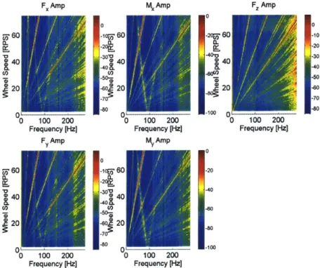
Magellan RW: Blocked Disturbance Amplitude Spectra . . . . 31

Magellan RW: Coupled Disturbance Amplitude Spectra . . . . 31

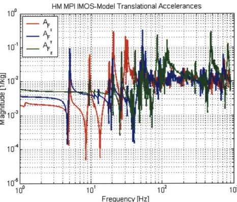
MPI FEM-Predicted Translational Accelerances. . . . . 33

MPI FEM-Predicted Rotational Accelerances. . . . . 33

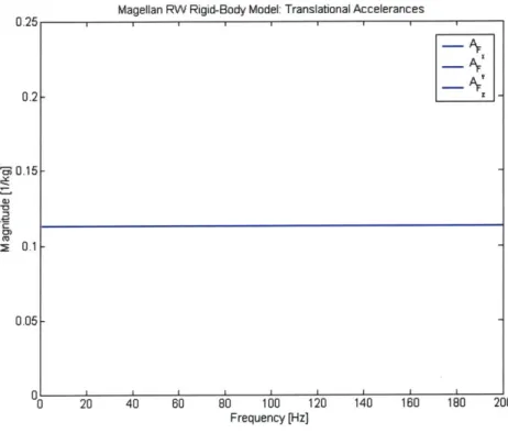
RW Rigid-Body-Model Translational Accelerances. . . . . 35

Shapes Used to Estimate the Magellan RW's Mass Moments of Inertia: (a) Cylinder and (b) Cone. . . . . 36

RW Rigid-Body-Model Rotational Accelerances. . . . . 37

Rigid Flywheel Model. . . . . 38

Measured Versus Predicted OPD Using Blocked RW Disturbances. . . 41

Measured Versus Predicted OPD Using Coupled RW Disturbances. . 42 Translational "rigid-RW, model3-MPI" Force Filters. . . . . 44

Measured Versus Predicted OPD Using Blocked RW Disturbances and "rigid-RW, model3-MPI" Filters. . . . . 44

Rotational "rigid-RW, model6-MPI" Moment Filters. . . . . 46

Measured Versus Predicted OPD Using Blocked RW Disturbances and "rigid-RW, model6-MPI" Force and Moment Filters. . . . . 46

"Rigid-gyro-RW, model6-MPI" Moment Filters: (a) Mx Filter and (b) My Filter. . . . . 48

Measured Versus Predicted OPD Using Blocked RW Disturbances and the "rigid-gyro-RW, model6-MPI" Force and Moment Filters. . . . . 48

xii LIST OF FIGURES

Figure 3.21 Measured Versus Predicted OPD Using Blocked RW Disturbance PSDs and CSDs (Without Force and Moment Filters). . . . . 50 Figure 4.1 Sample System: Pendulum Tube with Ball . . . . 65 Figure 5.1 Representative Model of One Spacecraft in an EMFF Array . . . . 75 Figure 5.2 Global Reference Frame, G, for Multiple-Spacecraft EMFF Array . . . 78 Figure 5.3 Typical Electromagnetic Coil Consisting of Multiple Windings of

Conduct-ing W ire . . . . 90 Figure 5.4 Schematic of the Electromagnetic Actuator Configuration in an EMFF Array

91

Figure 6.1 Geometry of Two-Spacecraft EMFF Array . . . 126 Figure 6.2 Local Curvilinear Coordinate Frame at Spacecraft A . . . 126 Figure 6.3 Pole-Zero Map for Two-Spacecraft EMFF Array, Using Geometric Values in

Table 6.1. . . . 153 Figure 6.4 Open-Loop and Closed-Loop Eigenvalues of the Linearized Design Model

163

Figure 7.1 Dynamic Simulation with Very Small Initial Conditions: State Responses 168

Figure 7.2 Dynamic Simulation with 10% Initial Condition on Dr: State Responses 169

Figure 7.3 Dynamic Simulation with 10% Initial Condition on Dr: Actuator Signals 169

Figure 7.4 Dynamic Simulation with 35% Initial Condition on Dr: State Responses 171

Figure 7.5 Dynamic Simulation with 35% Initial Condition on Dr: Actuator Signals 171

Figure 7.6 Dynamic Simulation with 40% Initial Condition on Dr: State Responses 172

Figure 7.7 Dynamic Simulation with 40% Initial Condition on Dr: Actuator Signals 172

Figure A. 1 F, Empirical Force Filter . . . 186 Figure A.2 _{M, Empirical Moment Filter. . . . 186} Figure D. 1 Linear Airtrack Used to Demonstrate Simplified Electromagnetic Formation

Control . . . 223 Figure D.2 _{dSPACE Virtual Control Panel Created for Airtrack System . . . 224} Figure D.3 Schematic of the Stable Airtrack Configuration . . . 227

Figure D.5 Figure D.6 Figure D.7 Figure D.8 Figure D.9 Figure D.10 Figure E.1 Figure E.2 Figure E.3

Schematic of the Unstable Airtrack Configuration . . . 230

Unstable Airtrack Pole-Zero Map . . . 230

Open- and Closed-Loop Step Responses of Stable Airtrack . . . 233

Open- and Closed-Loop Responses of Unstable Airtrack. . . . 234

EMFF Testbed Vehicle . . . 236

Angle-Tracking Results Using One Vehicle on the Planar Testbed . . . 238

Two Spacecraft Spinning Up About the Array Centerpoint . . . 242

Translation-Dependent Shear Force on Two Vehicles with Perpendicular M agnetic Dipoles . . . 244

TABLE 2.1 TABLE 3.1 TABLE 5.1 TABLE 5.2 TABLE 5.3 TABLE 5.4 TABLE 6.1 TABLE 6.2 TABLE 6.3

Generalized Input-Output Relationships Between a Load and Displacement, Velocity, and Acceleration. . . . . 21

Estimated Mass Moments of Inertia [kgm2] for the Magellan RW. . . 36

Summary of the Coordinates Defined for Spacecraft A and its Reaction W heel (RW -3) . . . . 80 Components of the Angular Velocity Vectors in Terms of Euler Angles 86 Generalized Coordinates for Spacecraft A and RW-3 . . . . 96 Generalized Speeds for Spacecraft A and RW-3 . . . . 97 Physical Parameters Used to Plot the Eigenvalues in Figure 6.3. . . . 153

State Penalties for LQR Control Design . . . 161 Actuator Penalties for LQR Control Design . . . 162

A, As _{Coil Cross-Sectional Area [m2]}

a1, a2, a3 Body-Fixed Coordinate Axes on Spacecraft A

bl, b2, b3 Body-Fixed Coordinate Axes on Spacecraft B

B, Magnetic Field due to Ma etic Moment of ith Spacecraft [T] CSD Cross Spectral Density [N /Hz]

DAQ Data Acquisition System DOF Degree(s) of Freedom

EM Electromagnet, Electromagnetic

EMFF Electromagnetic Formation Flight/Flying

er, e4, e, Spherical Coordinate Axes

eX, ey, e2 Global Coordinate Axes FEM Finite Element Model/Method FRF Frequency Response Function

Fr, F , FV Forces on Spacecraft, Resolved on Spherical Frame [N]

Fx, Fy, Fz Forces on Spacecraft, Resolved on Global Cartesian Frame [N]

F1, F2, F3 Forces on Spacecraft, Resolved on Body-Fixed Frame [N]

i Current Running Through Electromagnetic Coil [A]

I Mass-Moment of Inertia of Spacecraft A about Radial Axes [kg. m2

I _{Mass-Moment of Inertia of Spacecraft A about Spin Axis [kg. m2}2

I ,Reaction Wheel Mass-Moment of Inertia about Radial Axes [kg- m2 13

,

mA Spacecraft Mass [kg] mc Reaction Wheel Mass [kg]

MIT Massachusetts Institute of Technology MPI Micro-Precision Interferometer

n Number of States of the System

n, ns Number of Conductor Wraps around Electromagnet

OPD Optical Pathlength Difference PSD Power Spectral Density [N2/Hz]

rAG Position Vector of Spacecraft A [m]

r, *, Y Spherical Coordinates of the Position of Spacecraft A

RMS Root Mean Square RPM Revolutions per Minute

RW Reaction Wheel

RWA Reaction Wheel Assembly SIM Space Interferometry Mission SSL Space Systems Laboratory TPF Terrestrial Planet Finder

TM Motor Torque on Reaction Wheel [Nm]

T,., To, Ty Torques on Spacecraft, Resolved on Spherical Frame [Nm]

xviii NOMENCLATURE

Tx, Ty, Tz Torques on Spacecraft, Resolved on Global Cartesian Frame [Nm]

u Control Vector

x State Vector

XAO YAO ZAG Global Cartesian Coordinates of Spacecraft A XB0 YBO ZBG Global Cartesian Coordinates of Spacecraft B

xCA, yCA, zCA Position Coordinates of RW-3 with Respect to Spacecraft A

ci ith Euler Angle of Spacecraft A [rad]

Pg

yg ith Euler Angle of RW-3 on Spacecraft A [rad]

63 Rotation angle of RW-3 on Spacecraft A [rad] 63 Spin Rate of RW-3 on Spacecraft A [rad]

ft _{Magnetic Moment of Coil [A -m2]}

go Permeability of Free Space [T -m/A] $0 Nominal Spin Rate of Array [rad/s] 0 Spin Rate of RW [rad/s]

INTRODUCTION

1.1 Motivation

Space-based telescopes are an enabling technology that will allow us to observe solar sys-tems around neighboring stars, and will ultimately aid in the search for life beyond Earth. Telescopes in space avoid the atmospheric distortions that ground-based telescopes are subject to, and therefore allow us to see farther into space and gain better images of extra-solar planets. As space telescope technology continues to improve, we will answer more and more questions about the universe.

However, there are several design challenges associated with space-based telescopes. For instance, there is a trade between the angular resolution of a space telescope and its cost. A larger aperture provides improved angular resolution, but at the expense of an increased mass and volume. Hence the ideal telescope has as large an aperture as possible, within the limits of the given launch vehicle.

Space-based interferometry is a technology that has been proposed to provide the desired angular resolution, while maintaining a vehicle (or set of vehicles) that can be launched into space. An optical interferometer uses several separated apertures to collect light for scientific observation. The light from each aperture is then passed to a combiner, where an image is formed by interfering the light from the collectors. A set of separated aper-tures thus act as one large virtual aperture. Just as a monolithic telescope's angular

2 INTRODUCTION

tion i mproves w ith an i ncreased aperture s ize, an i nterferometer's r esolution improves with increased spacing between the separated apertures. Hence the ideal space interfer-ometer will be composed of multiple apertures separated by large distances.

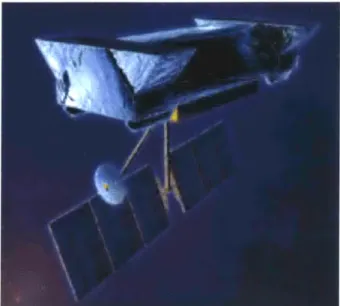
Two main architectures have been proposed for implementing space-based interferometry: a structurally connected platform, and a free-flying (formation flying) array of spacecraft. The former concept is shown in Figure 1.1, which depicts N ASA's forthcoming Space Interferometry Mission (SIM) [1]. SIM uses a 10-meter flexible truss platform to support the multiple apertures that compose the interferometer. There are both benefits and limita-tions of this architecture:

e The main benefit of this architecture is that the relative distances between the

apertures are fixed, to within the vibrational tolerances of the flexible boom. Hence there is no need for very coarse (on the order of meters) control of the relative spacing between apertures. Finer-level control may be implemented using optical delay lines, voice coils, and fast-steering mirrors [2, 3].

- The main limitation of this architecture is the relatively small (and fixed) baseline distance between the apertures; the aperture spacing is limited by the length of the boom, which is in turn limited by the volume of the launch vehicle fairing. Hence the angular resolution of this system is less than that of a system with a larger baseline.

- The main challenge of this architecture is the fine control of the distances between the apertures. Because the light from the collectors must be inter-fered to form an image, the optical pathlength of the light from each aperture must be controlled to within a fraction of the wavelength of the light. This nanometer-level precision must be maintained in the presence of on-board dynamic disturbances, such as imperfectly balanced, spinning reaction wheels, which c ause vibrations o ft he support structure. F or this reason, strict tolerances are placed on the magnitudes of vibration of such spacecraft, and detailed disturbance analyses and control design are required to ensure that deflections and vibrations are limited to acceptable levels for scientific data collection.

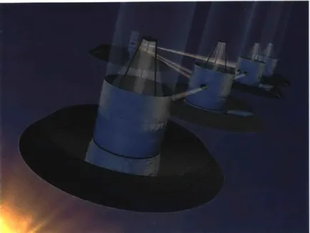
The free-flying concept for space-based interferometry is shown in Figure 1.2, which depicts a potential architecture for NASA's forthcoming Terrestrial Planet Finder (TPF) mission [4]. TPF is considering this formation flying interferometer architecture, as well as a structurally connected interferometer and a monolithic coronagraph. In the formation

Figure 1.1 NASA's Future Space Interferometry Mission (SIM)

flight architecture, four spacecraft act as collectors of light, and the fifth spacecraft acts as a combiner. Like the structurally connected interferometer concept, there are both bene-fits and limitations to this architecture:

. The main benefit of this architecture is the increased and variable baseline distance between the vehicles. TPF proposes a baseline between 75 meters and 1 kilometer, distances that are far greater than those possible with a structurally connected interferometer [5]. Further, the baseline is variable, and may be set to an optimal length for a given data collection mode.

- The main challenge of this architecture is the coarse level of control (on the order of meters and centimeters) needed to maintain the relative separation distances between the free-flying vehicles. Coarse control using thrusters raises several concerns, including the thermal and optical contamination due to the thruster plumes, as well as a mission lifetime limited by a finite thruster fuel supply.

1.2 Research Objectives and Approach

In this thesis, we address some of the dynamics and control challenges of both the struc-turally connected and formation flying interferometer concepts described above. We now discuss the research objectives and approach for each architecture.

4 INTRODUCTION

Figure 1.2 NASA's Future Terrestrial Planet Finder (TPF) Mission

1.2.1 Structurally Connected Interferometer

In Chapters 2 and 3, we consider the dynamics of a structurally connected interferometer. The primary challenge of such a system was described above. Namely, we are concerned with the vibrational tolerances of the support structure, and the resulting tolerances of the optical instruments. The goal is to maintain the optical pathlength difference (OPD) of the multiple arms of the interferometer to the nanometer level, with either passive damping or active control. We focus here on the dynamic analysis, rather than the control of this structure. Specifically, we develop an analysis method for determining the optical

perfor-mance of the system, even in the presence of on-board vibrational disturbance sources.

The result will be a toolbox that, given a set of dynamic disturbances and a model of the structural-optical system, predicts the resulting performance. The performance will then be assessed to determine whether the structure achieves the required jitter tolerances, and therefore whether the optical interferometer achieves sufficient dynamic stability to oper-ate successfully.

As discussed in detail in references [6, 7], the primary disturbance source anticipated for missions such as SIM is the on-board reaction wheel, used for attitude control. In [6], a

dynamic disturbance analysis method is developed that dynamically couples the reaction wheel to the spacecraft in order to predict the resulting system performance. The motiva-tion lies in the fact that reacmotiva-tion wheel disturbances are typically measured with the reac-tion wheel assembly "hardmounted" to a rigid surface, so that the interface loads are measured by load transducers while the flywheel spins. The problem with this measure-ment technique is that the boundary conditions of the hardmounted reaction wheel are not representative of the conditions when the wheel is fixed to the spacecraft. Hence the hard-mounted disturbances that are measured do not accurately represent the "coupled" distur-bances that occur when the wheel is fixed to the spacecraft.

To account for this, the coupled disturbance analysis method uses the hardmounted distur-bances as the input disturbance source to the structural-optical model, but first "corrects" them so that they represent the coupled disturbance loads that would occur if the reaction wheel were mounted to the spacecraft. As will be described in Chapter 2, this correction of the disturbance loads relies on estimates of the driving-point mobilities or accelerances of the spacecraft and the reaction wheel at their common interface points.

In this thesis, we build upon the disturbance analysis method developed in [6]. First, we increase the fidelity of the analysis method by accounting for the nonlinear gyroscopic stiffening dynamics of the spinning flywheel in the reaction wheel's accelerance model. Any improvement in results will allow us to assess the degree of gyroscopic stiffening of the wheel, as well as its influence on the system performance. Further, we validate the analysis methodology on representative hardware, the Micro-Precision Interferometer (MPI) testbed at NASA's Jet Propulsion Laboratory (JPL). As this testbed is a scale model of SIM, validating the analysis method on MPI will prove very useful.

Our approach is shown on the left-hand side of Figure 1.3. First, the coupled disturbance analysis method is reviewed. Then the gyroscopic accelerance model of the reaction wheel is developed and implemented. Finally, the method is validated on the MPI testbed,

6 INTRODUCTION

and we use the results to assess both the success of the analysis method and the impor-tance of reaction wheel gyroscopic stiffening on the system performance.

Approach

put1:

IPart

StructurAly Coiected

j

I

r

I

Figure 1.3 Research Approach

1.2.2 Formation Flying Interferometer

In Chapters 4-7, we consider the dynamics and control of a formation flying interferome-ter. The primary challenge of such a system was described above. Namely, we seek a method for the coarse control of the relative distances and the attitudes of the spacecraft in an array, and we would like to achieve this without the use of thrusters (in order to elimi-nate the contamination they cause and to extend the lifetime of the mission). We propose the use of electromagnetic actuators, whereby each spacecraft is equipped with a set of electromagnets, and the relative distances between the vehicles are controlled using the

D eve I o 1,7-7 1111111i FIgid bodV dyndtirl-s mode', as;nq rM arttl(1101% L I I DN111rhance andilpis Inelhod lut flexible

body and IMA

interaction forces of the magnetic fields of the vehicles. We refer to this concept as elec-tromagnetic formation flight (EMFF).

The EMFF concept is promising for many reasons. First, it eliminates thermal and optical contamination issues associated with thruster plumes. Second, it has the potential to greatly increase the mission lifetime, since it relies on a renewable energy source (electri-cal power from solar arrays), rather than a finite fuel supply. Further, if superconducting wires are used to form the electromagnets, the system will sustain very small resistive losses, and therefore will require only a very small amount of power. Finally, EMFF con-trols the relative separation distances between vehicles, which is the metric of importance in space interferometry applications. Hence valuable effort is not spent controlling the absolute degrees of freedom of each vehicle, as with thrusters.

While EMFF has many benefits, it also has many challenges. First, the electromagnetic forces are spatially nonlinear. The forces b etween any two electromagnets (EMs) are inversely proportional to the fourth power of the separation distance. Hence EMs may produce very strong forces when they are near each other, and very weak forces when they are farther apart. Also, the control is coupled. Every powered EM affects every other powered EM in the array, so a systematic method should be used to derive the control law.

As EMFF is a newly proposed technology, we focus on demonstrating the feasibility of the dynamics and controls of an EMFF system. Our approach is shown on the right-hand side of Figure 1.3. First, we develop from first principles a high-fidelity model of the sys-tem. In addition to modeling the nonlinear actuator terms, we model the nonlinear dynam-ics of each vehicle in the array, as well as the nonlinear gyroscopic stiffening dynamdynam-ics of its spinning reaction wheel. Next we linearize the dynamics about a nominal trajectory, and the resulting linearized equations of motion serve as a design model. We analyze the linearized dynamics to determine whether the system is stable, and whether it is controlla-ble. The controllability of the system is a key factor to determining the practicability of EMFF. Next we design a linear, optimal controller for the system using the design model,

8 INTRODUCTION

and we implement the controller with the nonlinear equations of motion (the evaluation

model) to form the closed-loop nonlinear dynamics. Finally, we simulate the closed-loop

dynamics in order to assess the effectiveness of the EMFF concept. Initial hardware dem-onstrations are also presented in Appendix D, and recommendations will be made for higher fidelity hardware demonstrations.

1.3 Literature Review

1.3.1 Review of Flexible Body Coupling Literature

The derivation of the coupled disturbance analysis method in this thesis was motivated by the fact that the SIM integrated modeling team at NASA's JPL has relied on a decoupled disturbance analysis method that generally overpredicts their coupled measurements. Ref-erences [8] and [9] describe the decoupled method used at JPL.

In an attempt to correct the overprediction by the decoupled method, Ploen [10] developed a "force filter," which modifies the hardmounted forces so that they resemble the coupled forces. Although this was the first attempt within the SIM integrated modeling group to account for dynamic coupling between a structurally connected interferometer and its reaction wheel disturbance source, this method is very limited and invokes several approx-imations. For instance, it modifies only the hardmounted disturbance forces, and not the torques. Also, the force filters derived by Ploen assume that the accelerance matrix of a body is purely diagonal, and therefore that cross-accelerance terms do not exist. In reality, this holds true only in a very limited number of cases, and it is an approximation for most bodies. Reference [10] does provide a very clear, systematic derivation for the coupling theory, and provides a nice nomenclature (the "force filter" terminology) that we will adopt here.

Simultaneous with the work of Ploen, Elias [6] developed a full matrix coupling method, where the matrix accelerances of each body are taken into account (including

cross-accelerance terms). This results in a 6 x 6 loadfilter matrix, which is used to transform the hardmounted loads (forces and torques) into the equivalent coupled loads.

The work in this thesis will expand upon [6] by including the nonlinear, gyroscopic stiff-ening dynamics of the reaction wheel in the wheel's accelerance model. We use the "fil-ter" notation from [10], and expand upon this concept to include full matrix load filters. Finally, we validate this method on representative hardware and draw conclusions about which terms are influential, and which may be neglected without significantly altering the results of the analysis.

1.3.2 Review of Formation Flight Literature

Formation flight has recently become a key research interest among the aerospace com-munity because of its many applications, including space interferometry, earth observa-tion, and synthetic aperture radar.

A great deal of research has been done in the MIT Space Systems Laboratory to demon-strate formation flight on a hardware testbed. The SPHERES project [11] has evolved from a two-dimensional, ground-based laboratory experiment to one being tested in a zero-gravity, three-dimensional environment, both on NASA's KC-135 aircraft and in the future on the International Space Station (ISS). This testbed has demonstrated successful formation flight maneuvers, including leader-follower tracking and docking. The SPHERES Guest Scientist Program will allow engineers from around the world to upload algorithms to the vehicles while they are on the ISS. This will add a great deal to our cur-rent understanding of formation flight control algorithms.

Similar hardware-based demonstrations have b een performed at JPL, UCLA, Stanford, and the NASA Goddard Space Flight Center. All of these testbeds assume the use of thrusters to control the relative positions of the spacecraft. Open areas of research include the use of microthrusters, Micro-Electro-Mechanical Systems (MEMS), pulse plasma thrusters (PPTs), and colloid microthrusters [12].

10 INTRODUCTION

In addition to hardware demonstrations, much theoretical work has been done in the area of formation flight dynamics and control for spacecraft in deep space. Wang et. al. [13] present a formulation for the rigid-body dynamics of a multi-spacecraft spinning array, modeling each vehicle as a lumped mass and inertia. A similar approach was taken by Smith et. al. [14], who investigate various control topologies and their associated stability properties.

While all the above references assume a traditional actuation method, such as thrusters, for control of the relative spacecraft separation distances, Kong et. al. [2, 15] investigate the use of electromagnets for relative position control. In [15], several trade studies are presented, demonstrating that the required mass and power of EMFF systems are compa-rable to or more attractive than traditional propulsion methods. Reference [2] also investi-gates the controllability of non-rotating EMFF arrays and draws conclusions about the necessary electromagnetic topologies for such systems to be controllable.

Like Kong et. al., we extend the previous work by focusing on the use of electromagnets as the relative position actuators of the array. As described above, eliminating the use of thrusters offers several benefits, and we attempt to demonstrate the feasibility of this novel actuation method from a dynamics and controls perspective. Specifically, we extend the research in references [2, 15] by developing a higher fidelity, nonlinear dynamic model of an EMFF system. We model the spacecraft-reaction wheel system as a system of two rigid bodies that can rotate relative to one another about the reaction wheel's spin axis. Model-ing the dynamics in this way allows us to capture the nonlinear gyroscopic dynamics asso-ciated with the reaction wheel's spinning. As we will find in Chapter 5, the reaction wheels of a rotating array may store a significant amount of angular momentum, and therefore their nonlinear dynamics should be considered. Further, we analyze the system's dynamics in its mode of scientific observation (rotation of the entire array about its center point), and we assess the control possibilities for such a system via analysis and simula-tion.

1.4 Thesis Overview

As shown in Figure 1.4, this thesis is divided into two parts. Chapters 2 and 3 discuss the dynamics of a structurally connected space interferometer, while Chapters 4-7 discuss the dynamics and control of an electromagneticformation flying space interferometer.

Chapter 2:

-Introduction of the Coupled Disturbance Analysis Method

Chapter 3:

h4i- Validation of the Coupled Disturbance Analysis Method on the MPI testbed at JPL

Figure 1.4 Thesis Overview

In Chapter 2, the theory for a disturbance analysis method that accountsfor the structural

dynamic coupling between a flexible body and its disturbance source is introduced. In

Chapter 3, the hardware and experimental configurations used to validate the coupled dis-turbance analysis method are described in detail. The experimental results are then pre-sented for comparison with the predictions, so that the effectiveness of the analysis method may be assessed.

In Chapter 4, Kane's method for the derivation of a system's equations of motion is reviewed in detail. Kane's method is then applied in Chapter 5 to derive the nonlinear equations of motion for an electromagnetic formation flying array with an arbitrary num-ber of spacecraft. Expressions are given for the electromagnetic forces and torques applied to one spacecraft by another. Also, the nonlinear gyroscopic dynamics associated

12 INTRODUCTION

with the spinning reactions wheels are captured in the model, along with their effect on the attitude dynamics of the spacecraft.

In Chapter 6, the nonlinear equations of motion are linearized for a two-spacecraft system about a nominal trajectory. The linearized equations are analyzed for stability and control-lability, and a linear optimal controller is designed. The controller is implemented into the nonlinear equations of motion, and the resulting closed-loop dynamics are simulated in

Chapter 7.

Finally, a summary and a list of key contributions in this thesis are presented in Chapter 8, along with recommendations for further development of this work.

STRUCTURAL DYNAMIC COUPLING

THEORY

2.1 Introduction

NASA's future Space Interferometry Mission (SIM), depicted in Figure 1.1, will be the first space-based optical interferometer. With optics mounted to its flexible truss struc-ture, SIM must achieve nanometer-level stability requirements in the presence of on-board disturbances. The primary disturbance source anticipated for SIM is the reaction wheel (RW), a spinning flywheel assembly used for attitude control. In order to ensure mission success, a disturbance analysis method must be developed to predict SIM's on-orbit per-formance in the presence of RW disturbances.

RW disturbances are typically measured in a "blocked" or "infinite-impedance" configu-ration, in which the RW is hardmounted to a rigid surface and its interface is constrained to have zero motion. The RW is spun, and a load transducer is used to measure the result-ing disturbance loads at the interface. While this method provides well-defined and repeatable b oundary conditions, they are not an accurate representation of the coupled boundary conditions that occur when the RW is mounted to a structure. In other words,

the blocked RW d isturbances d iffer from t he c oupled d isturbances t hat w ould a ctually

exist at the spacecraft-RW interface if the two bodies were coupled together.

In this chapter, we present a modeling methodology to predict the dynamic performance of a flexible structure in the presence of on-board RW vibrational disturbances. Two

STRUCTURAL DYNAMIC COUPLING THEORY

bance analysis methods are presented: a decoupled method and a coupled method. In the decoupled method, the blocked RW disturbances are propagated through a spacecraft

fre-quency response function (FRF) to predict the resulting spacecraft performance. In the

coupled method, "load filters" are used to correct the blocked disturbances for the

artifi-cial boundary conditions imposed on the RW during disturbance testing. The filters, which rely on estimates of the RW and spacecraft interface accelerances, are used to "transform" the blocked RW disturbances into the corresponding coupled disturbances. The coupled disturbances are then propagated, in place of the blocked disturbances, through a spacecraft FRF to predict the coupled performance.

The decoupled and coupled methodologies will be presented in this chapter. First, the decoupled method is presented in Section 2.2. In Section 2.3, motivation is provided for the derivation of the coupled disturbance analysis method, and the coupled analysis method is described in detail. Finally, a summary and conclusions are presented in Section 2.4. In the following chapter, both methods will be validated by experimental data from the Micro-Precision Interferometer (MPI) testbed at NASA's Jet Propulsion Labora-tory (JPL).

2.2 Decoupled Disturbance Analysis Method

The decoupled disturbance analysis method is based on a simple frequency-domain

input-output principle. The performance metric, Z, of a flexible structure is related to the input disturbance source, F, as:

Z(o, Q) = GZF(o)F(o, n) (2.1)

where GZF is the FRF of the structure, o represents frequency (in units of radians per sec-ond), and Q represents the reaction wheel spin rate (in units of radians per second). Notice that the disturbance, F, is a function of both frequency and reaction wheel spin rate, and hence the performance metric, Z, is also a function of frequency and wheel spin rate. For a structural-optical system, such as a structurally connected interferometer, Z may be 14

defined either as a mechanical performance metric, such as the relative displacement of two points, or as an optical performance metric, such as the optical pathlength difference (OPD) between various light paths within the interferometer.

If we are considering a number, p, of performance metrics, then Z is the p x 1 predicted

performance vector. Since the disturbance source is a reaction wheel producing three

dis-turbance forces and three disdis-turbance moments, F is a 6 x 1 disdis-turbance load vector. Finally, GZF is the p x 6 FRF of the structure, relating the six disturbance loads at the RW-mounting location on the structure to the structure's p performance metrics.

Post-multiplying each side of Equation 2.1 by its complex-conjugate transpose and taking the expectation allows us to write the analysis equation in terms of spectral density matri-ces, which are a useful form for implementing experimental data. This yields:

*zz( m, 0) = GZF( o))FF(o), Q)GZ(*) (2.2)

where [.]*T denotes a complex-conjugate transpose operation, Dzz is the p x p predicted performance spectral density matrix, and OFF is the 6 x 6 RW disturbance spectral den-sity matrix, with disturbance power spectra as diagonal components and cross-spectra as off-diagonal components.

If we have a single performance metric of interest, so that p = 1 and Z is a scalar, the root mean square (RMS) of the performance metric can then be calculated for a given reaction wheel spin rate, Q, as:

= zaxzz(o((, Q)do (2.3)

Wmax

When Z is a vector containing more than one performance metric, az is a matrix whose diagonal components are the scalar RMS functions of the performance metrics contained

STRUCTURAL DYNAMIC COUPLING THEORY

In the case that the diagonal terms of OFF, or power spectral densities (PSDs), dominate the off-diagonal terms, or cross spectral densities (CSDs):

(FF ' VFjF1 , l #j (2.4)

then OFF may be approximated as a diagonal matrix, and Equation 2.2 reduces from a fully populated matrix equation to a simple summation of diagonal terms:

6

Oz o,) ~ (DFF(o), Q)|GzF( () 2 _(2.5)

j= 1

It is important to note that Equation 2.2 represents a decoupled disturbance analysis method, since the disturbance loads are usually measured in a blocked configuration (denoted OFF, b) and are then substituted for the disturbance loads (DFF) in Equation 2.2. Clearly OFF, b differs from the loads that occur when the RW is mounted to the spacecraft (denoted OFF, c). We will account for this discrepancy in the following section by deriv-ing a relationship between the blocked and coupled loads.

2.3 Coupled Disturbance Analysis Method

2.3.1 Motivation for Coupled Analysis Method

The remainder of this chapter is motivated by the fact that there is often a discrepancy between measured performances and those predicted by the decoupled analysis method presented above. For instance, performance predictions for the MPI testbed at JPL have been found to consistently overbound experimental measurements when calculated using Equation 2.5 [16]. The degree of discrepancy is not acceptable, since accurate perfor-mance predictions will be required to ensure the success of future NASA missions, such as the Space Interferometry Mission, prior to assembly and launch.

The discrepancy has been, up to now, attributed to two primary factors: 16

- the decoupled nature of the disturbance analysis method described in Equa-tion 2.5.

- the approximation made by Equation 2.4, yielding Equation 2.5 as a simpli-fied representation of Equation 2.2.

The first concern is addressed in this chapter, and the latter is addressed in Chapter 3, where we will use experimental data to investigate the validity of the approximation in Equation 2.4.

In the remainder of this chapter, we propose a coupled disturbance analysis method to improve upon the decoupled method presented in Section 2.2. In propagating blocked RW disturbances through a structural FRF, the decoupled method neglects the structural

dynamic coupling between the flexible structure and the RW. Our goal is thus to correct

the mismatch in RW disturbance-testing boundary conditions by applying a coupling the-ory to the performance predictions. Reconciling the measured and predicted perfor-mances will affirm our ability to predict a spacecraft's on-orbit dynamic behavior prior to

flight.

2.3.2 The Load Filter

In order to correct the mismatch of boundary conditions that occurs in blocked RW distur-bance testing, a loadfilter matrix, Gf, may be used to relate the measured blocked RW disturbances, Fb, with the "true" coupled disturbances, F , [16, 6]:

F(o, 0) = G/co, n)Fb(o, Q) (2.6)

where o represents frequency, and i represents the reaction wheel spin rate (in units of radians per second). Recall the loads, Fb and Fc, are 6 x I matrices, each consisting of the three disturbance forces and three disturbance moments imparted by the RW with the given boundary conditions (blocked or coupled, respectively). Therefore the load filter,

18 STRUCTURAL DYNAMIC COUPLING THEORY

By post-multiplying each side of Equation 2.6 by its complex-conjugate transpose and manipulating slightly, we can express Equation 2.6 in terms of spectral density matrices:

OFF, c(o, 0) = Gfo, Q) DFF b(o, Q)G f(o, Q) (2.7)

where the [-] operation was defined in Section 2.2.

The goal is to now define the load filter, G, which provides a relationship between the blocked and coupled loads. Once that relationship is defined, we will have the ability to "filter" any set of blocked loads into the corresponding coupled loads for use in a coupled disturbance analysis.

By studying the derivation in references [6, 17] and adopting the notation used in [10], we can define the load filter matrix as:

-I -1

Gfjo, Q ) = [ I+ A-, 0), Q As~) (2.8)

where I is the 6 x 6 identity matrix, AR W is the 6 x 6 driving-point accelerance matrix of the RW at its interface point with the structure, and As is the 6 x 6 driving-point acceler-ance matrix of the flexible structure at its interface point with the RW.1 Notice that the RW's accelerance matrix is dependent upon the wheel's spin rate, since the spinning of the wheel causes a nonlinear, gyroscopic stiffening effect and thereby influences the wheel's accelerance. Therefore the load filter matrix, Gf, is also dependent upon the RW's spin

rate.

1. The driving-point accelerance is a complex, frequency-dependent ratio of co-located acceleration and

force at the interface, or "driving point" of a body. It is the inverse of the driving-point apparent mass. For more information, see reference [18].

A simplified version of the load filter matrix in Equation 2.8 was introduced in reference [10]. A scalar force filter was defined to relate the measured blocked RW forces with the "true" coupled forces:

F i(co) 1

Gf

Fb,1() + AS,ii(O)

ARW,ii (")

where i = 1, 2, 3 refers to the x, y, and z axes, respectively, Gf ii is a "force filter" along the ith axis, Fcj is the Fourier transform of the coupled interface force along the ith axis, Fbj is the Fourier transform of the measured blocked force along the ith axis, Asjg is the spacecraft's point accelerance along the ith axis, and ARWii is the RW's driving-point accelerance along the ith axis. Note that this force filter is an approximation of the load filter in Equation 2.8 in two ways:

1. The force filter is not dependent on the wheel's spin rate, Q, and therefore does not capture the effect of the wheel's gyroscopic stiffening on its accelerance. (In other words, ARW(o, Q) is approximated as A RW(O), so that Gj it is independent of the RW's spin rate.) While this may be a fair approximation at low wheel speeds, it may not hold true for higher wheel speeds.

2. The force filter assumes that the accelerances of the RW and spacecraft are diagonal matrices

(with

The concept of the scalar force filter was expanded in [16] to include a similar "moment filter," which may be expressed as:

f it(Mo)(=O) ' i = 4,5 6 (2.10)

Mb, Mo) + s±it(O)

AR W,ii&)

where i = 4, 5, 6 refers to rotations about the x, y, and z axes, respectively, Mcji is the

20 STRUCTURAL DYNAMIC COUPLING THEORY

transform of the measured blocked moment along the ith axis, Asjg is the spacecraft's driv-ing-point rotational accelerance about the ith axis, and ARWii is the RW's drivdriv-ing-point

rotational accelerance about the ith axis.

Table 2.1 lists the generalized input-output relationships between a load, F, imparted on a body and its resulting p osition, velocity, and a cceleration:

Q, Q,

Q,

[18]. (Where there is more than one acceptable term, the more common term is shown in bold.) From this table, it is clear that accelerance, A, is simply a derivative of mobility, Y

[6]:

A (o) = _ i)o -jo = Y(o) (2.11)

F(o) F(o)

and thus that the ratio of two bodies' accelerances is equivalent to the ratio of their

mobil-ities:

Asi _ # s1ii _Ys,ii

ARW~ii j)RWii YRWii

Hence the scalar force and moment filters in Equations 2.9 and 2.10, respectively, can be formed using the ratio of spacecraft and RW accelerances or mobilities:

;o)- 1 + -1( , 1, 2, 3 (2.13)

Fb, ifc) +Asjii(0)_ 1 sjit(()

ARW~i((o) YRWH(CO)

___ 1 + 1 i+

M, M(O) II

Gf, ii(o)M= 1 + A-₁i@O) 1 i = 4, 5, 6 (2.14)

Mbif)Asiifo) Ysi0))

2.3.3 Coupled Analysis Method

Recall from Equation 2.2 the input-output relationship used as the basis for the decoupled disturbance analysis method, where blocked disturbance PSDs, CFF, b(o, 0), are used to

TABLE 2.1 Generalized Input-Output Relationships Between a Load and Displacement, Velocity, and Acceleration.

Response/Load Ratios Load/Response Ratios

Receptance,

a(o) Admittance, Dynamic Stiffness

F(o) Dynamic Compliance, a(O) Q(O)

Dynamic Flexibility

Y(o) - F() Mobility Z(o) F&() Mechanical Impedance

F(w) Qo

Q(mO) Accelerance, I _ F(o) Apparent Mass,

F(o) Inertance A (o) Dynamic Mass

represent the disturbance PSDs, 1_{FF(o, Q), that are applied to a spacecraft. If instead,}

we use the coupled disturbance PSDs, OFF, c(o, Q), as expressed in Equation 2.7, to rep-resent the disturbance PSDs applied to the spacecraft, we will obtain a coupled

distur-bance analysis equation analogous to the decoupled Equation 2.2:

(D *T *T

zzco, Q) = GZF(o)Gf(o, Q) 1

FFb(o, Q)G (o, Q)GZF(w) (2.15)

Comparing Equations 2.2 and 2.15, we see that the load filter, Gf, effectively "filters" the loads measured in the blocked configuration (GFF, b) to represent the loads that would occur at the coupled spacecraft-RW interface (DFF, ). For this reason, the name "force filter" was originally coined [10], although it is replaced by "load filter" here, to represent the matrix, Gf, that filters both forces and moments.

Also recall the assumption in Equation 2.4 that the disturbance PSDs dominate the CSDs, allowing us to approximate Equation 2.2 as Equation 2.5. Following this same assump-tion, the coupled disturbance analysis method in Equation 2.15 can be approximated as:

6

(Dzzf*(, Q);~ =)1Gf, DFjF,, b(o, U(o)1 GZF

j=

STRUCTURAL DYNAMIC COUPLING THEORY

where Gf g are the diagonal components of the load filter matrix in 2.8. Analogous to Equation 2.7, the terms '1 FF, b(o, Q)|Gf 2(o) represent the filtered or coupled distur-bance PSDs, DF;F,, (co, D). Hence using Equation 2.16 in place of Equation 2.5 effec-tively transforms the experimentally-measured blocked RW disturbances into the disturbances that would occur at the coupled spacecraft-RW interface.

Further, if only scalar accelerances are available and matrix accelerances are not, Equation 2.16 may be further simplified as:

6 2 2

Qzfo ) "Zt Z (FF,, b(0 ;i )GZFj I) 7))

j= I

where Gf ii represents the scalar force and moment filters in Equations 2.13 and 2.14, respectively. As explained above, Gf h and k it are equivalent only if the accelerance matrices of the spacecraft and RW are diagonal (with off-diagonal components equal to

zero). Otherwise, Gjf it is an approximation of Gf .

One final simplifying assumption may be made. Since translational accelerances are sim-pler to measure experimentally (using accelerometers) than rotational accelerances, there may be cases in which force filters are available, but moment filters are not. In this case, Equation 2.17 is further approximated by:

Czzf* C" FiFi, b 2 GZF 2lf i 1(2.18)

+ GFFi, b(W,)|GZF 2

j=4

where the moment filters have been set to unity. This equation represents a compromise between the decoupled and coupled methods, since it is coupled in the translational degrees of freedom (forces), but decoupled in the rotational degrees of freedom 22

(moments). With only translational accelerances (and therefore force filters) available, this approximation may still yield an improvement over the decoupled analysis method.

2.4 Summary and Conclusions

In this chapter, we have:

" provided the motivation for a disturbance analysis method to predict the dynamic performance of a flexible space structure in the presence of reaction wheel vibrational disturbances.

- presented a decoupled disturbance analysis method.

- provided the motivation for a coupled disturbance analysis method.

- derived a coupled disturbance analysis method and highlighted the differ-ences from the decoupled method.

The primary contribution has been the derivation of a new, coupled disturbance analysis method. This method will improve our prediction capability for precision space missions, such as NASA's forthcoming Space Interferometry Mission (SIM), which has very strict tolerances on its optical performance metrics. With this new, high-fidelity method of pre-dicting SIM's optical on-orbit performance prior to launch, we will be able to accurately assess SIM's behavior and to ensure the success of the mission and its ability to achieve scientific goals. The coupled disturbance analysis method has been adopted by the SIM integrated modeling team and may prove to be an invaluable analysis tool in future

preci-sion-space-telescope missions.

In the following chapter, we will demonstrate and validate both the decoupled and coupled disturbance analysis methods using representative hardware.