HAL Id: hal-01692110
https://hal.archives-ouvertes.fr/hal-01692110
Submitted on 20 Oct 2018
HAL is a multi-disciplinary open access
archive for the deposit and dissemination of
sci-entific research documents, whether they are
pub-lished or not. The documents may come from
teaching and research institutions in France or
abroad, or from public or private research centers.
L’archive ouverte pluridisciplinaire HAL, est
destinée au dépôt et à la diffusion de documents
scientifiques de niveau recherche, publiés ou non,
émanant des établissements d’enseignement et de
recherche français ou étrangers, des laboratoires
publics ou privés.
Theory Applied to Cable Harnesses
Sofiane Chabane, Philippe Besnier, Marco Klingler
To cite this version:
Sofiane Chabane, Philippe Besnier, Marco Klingler. An Embedded Double Reference Transmission
Line Theory Applied to Cable Harnesses. IEEE Transactions on Electromagnetic Compatibility,
Insti-tute of Electrical and Electronics Engineers, 2018, 60 (4), pp.981-990. �10.1109/TEMC.2017.2754470�.
�hal-01692110�
Abstract—In this paper, an embedded double reference transmission line theory (EDRTLT) is presented. This approach is based upon taking an arbitrary wire among the 𝒏 wires
constituting the harness and considering it as an internal reference conductor. Then the initial transmission line of 𝒏 wires
above a ground reference is split into two coupled subsets of wires. The internal subset is composed of 𝒏 − 𝟏 wires with the
internal reference wire as the return wire. The per unit length (p.u.l.) parameters of this internal transmission line are calculated with respect to this internal reference wire. They do not depend on the ground reference. The external subset is composed of only the internal reference wire with the ground plane as a reference. As a result, any change of relative position of the bundle and the ground reference involves the p.u.l. calculation of a mono-conductor transmission line. This double reference transmission line theory is shown to be equivalent to the classical single reference approach and the corresponding p.u.l. parameters are approximately retrieved from those of the single reference transmission lines to form the EDRTLT. The results obtained by this theory are in good agreement with those obtained from the single reference case where all p.u.l. parameters are directly calculated using the ground plane as a single reference. The main advantage provided by the EDRTLT is to reduce the complexity of analysis of the bundle-to-ground interaction.
Index Terms—automotive, electromagnetic compatibility (EMC), cable harnesses, crosstalk, high frequencies, electromagnetic interference, multi-conductor transmission lines, radiation, transmission line theory (TLT).
I. INTRODUCTION
arnesses are key sub-systems from an EMC perspective in various domains such as automotive, aeronautic or telecommunication industries. Indeed, they can receive, conduct and radiate electromagnetic energy. Ideally, their effect should be assessed with a rigorous resolution of
Manuscript submitted on Month Day, Year. This work was supported by the French C.N.R.S. and Groupe PSA.
S. Chabane was with the Institute of Electronics and Telecommunications of Rennes (IETR), UMR C.N.R.S. 6164, INSA of Rennes, 20 avenue des Buttes de Coësmes, CS 14315, Rennes Cedex 35043, France. He is now with Safe Engineering Services & technologies ltd, 3055 Boulevard des Oiseaux, Laval, Quebec, H7L 6E8, Canada(e-mail: [email protected]).
P. Besnier is with the IETR UMR C.N.R.S. 6164, INSA of Rennes, 20 avenue des Buttes de Coësmes, CS 14315, Rennes Cedex 35043, France (e-mail: [email protected]).
M. Klingler is with Groupe PSA, Centre Technique de Vélizy, DQI/DRIA/DSTF/SIEP, 2 route de Gisy, 78943 Vélizy-Villacoublay Cedex, France (e-mail: [email protected]).
Maxwell's equations, but this approach is simply impossible due to time and memory requirements to handle so many of them. Thus, a well-known and often used alternative consists in applying the transmission line theory (TLT) accounting for the presence of a nearby grounding structure[1].Nevertheless, this theory, being just an approximate solution derived from Maxwell's equations, is limited by its assumptions [2] based mainly on the condition that the distance between the transmission line and its return path should be much smaller than the minimum significant wavelength of the incident electromagnetic field. This condition is not fulfilled in areas where cable paths are at a greater distance from the chassis. A typical situation is that of the Fig. 1. This will be the investigation case study throughout this paper. Moreover, the classical TLT is not valid at resonant frequencies even when its applicability conditions are satisfied. In the recent years, some techniques modifying the transmission line (TL) equations have been developed in several fields of application [3]–[7]. The main goal of these models is to be applicable beyond the validity limits of the classical TLT. However, most of these solutions require an entire new software development or are based on time consuming iterative methods.
Fig. 1. A typical piece of wiring system in a vehicle
Recently, the authors have also developed a new TL model that keeps the simplicity of the classical TLT equations and leads to very satisfactory results in high frequency regions and even at resonances. This model (called the modified enhanced transmission line theory, METLT) is valid in the case of a single wire as well as for a multi-conductor transmission line [8]–[10]. Its main particularity is that its p.u.l. parameters are frequency dependent, account for radiation, and its equations may be resolved using classical TLT equations. This makes it a low cost and non-intrusive solution, since it only requires an implementation of a new plug-in that calculates the corrections applied to the classical p.u.l. parameters.
However, for any height variation of the bundle over a ground plane, all p.u.l. parameters have to be recalculated. Moreover, if the ground reference possesses a complex geometry, the determination of the Green's functions yielding to the determination of p.u.l. parameters require the use of
An Embedded Double Reference Transmission
Line Theory Applied to Cable Harnesses
Sofiane Chabane, Philippe Besnier, Senior Member, IEEE, and Marco Klingler, Member, IEEE
full-wave resolution. Any change of geometry of the surrounding ground reference requires estimating each element of the p.u.l. matrices involving each wire and each pair of wires of the bundle. In the frame of the classical TLT or of the METLT, calculating the p.u.l. parameters from an intrinsic description of the p.u.l. parameters of the bundle would provide a huge simplification.
This paper is dedicated to the presentation of such an approach based on the embedded double reference transmission line theory (EDRTLT). This theory applies for a harness which height or distance over the reference ground plane is much greater than its overall cross-section and even if it is not much smaller than the wavelength, applying the METLT. Our method consists in decomposing the initial 𝑛conductor transmission line into two coupled subsets, a𝑛 − 1 conductor and a single conductor transmission line. The 𝑛 − 1 conductor transmission line uses the remaining conductor of the bundle as a local reference. The single conductor transmission line is composed of this remaining conductor and the surrounding ground reference. We show that the resulting single-reference transmission line p.u.l. parameters may be calculated from the knowledge of p.u.l. parameters of the double-reference system of transmission lines (and vice versa). Furthermore, the p.u.l. parameters of the 𝑛 − 1conductor transmission line have their own classical (quasi-static) expressions. The p.u.l. parameters of the single conductor transmission line may be calculated from quasi-static or modified enhanced p.u.l. parameters expressions according to the height of the bundle over the ground plane. In case of a complex shaped ground plane, the calculation of the p.u.l. parameters is reduced to that of a single wire only.Note that this paper does not discuss the validity of the transmission line approximation using classical TLT equations or METLT. It aims at introducing and validating the EDRTLT in comparison with direct evaluations of TLT / METLT using a single reference.
The rest of the paper is organized as follows. Section II introduces the single and double reference transmission line systems and their relationships in terms of p.u.l. parameters. We specifically illustrate that the single-reference p.u.l. parameters may be retrieved from the double-reference ones. Section III is dedicated to the p.u.l. parameters evaluation. In the frame of the METLT, the double-reference transmission line parameters are established for an𝑛-conductor bundle at a constant distance over a ground plane. These expressions are derived for a bundle whose height over the ground plane is much larger than its diameter. Section IV validates this evaluation based upon the comparison of the single-reference p.u.l. parameters evaluated in two different ways: i) a direct evaluation from a single reference transmission line ii) an indirect evaluation from the parameters of the double-reference transmission line. A validation is proposed in Section V for a crosstalk scenario between two wires, and Section VI provides a final discussion.
II. FROM A SINGLE TO A DOUBLE VOLTAGE REFERENCE
A. Single reference
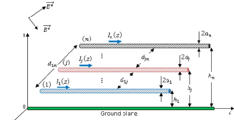
Consider a system of 𝑛 lossless uniform wires above an infinite PEC ground plane illuminated by an external electromagnetic field (Fig. 2). Every wire 𝑖 with 𝑖 ∈ [1, 𝑛]has a radius 𝑎𝑖, is at a height ℎ𝑖 above the ground plane and
separated from another wire𝑗 by a distance 𝑑𝑖𝑗 (Fig. 3). Wires
are parallel to the Oz axis. According to the thin wire hypothesis, voltages and currents only depend on the z spatial variable. This dependence in z will be implicit in all formulas throughout the paper
Fig. 2.Geometry of a system of (n+1) conductors
Fig. 3.Geometry of study
When the ground plane is considered as the unique return conductor, the constitutive equations of this system correspond to the geometry depicted in Fig. 4. Superscript ‘SR’ is used in the following equations to indicate that all quantities such as voltages, currents, impedances, admittances are calculated with the ground plane as a single reference. Transmission line theory coupled equations are given by [10]:
𝑑 𝑑𝑧[𝑉 𝑠(𝑆𝑅)] + [𝑍(𝑆𝑅)][𝐼(𝑆𝑅)] = [𝐸 𝑧 𝑒(𝑆𝑅) ] (1) and 𝑑 𝑑𝑧[𝐼 (𝑆𝑅)] + [𝑌(𝑆𝑅)][𝑉𝑠(𝑆𝑅)] = 0, (2) where
[𝑉𝑠(𝑆𝑅)(𝑧)]is a column vector of individual voltages
differences 𝑉𝑖𝑠(𝑆𝑅)(𝑧)between wire i and the ground plane. [𝐼(𝑆𝑅)(𝑧)]is a column vector of individual currents
𝐼𝑖𝑠(𝑆𝑅)(𝑧)on wire i [𝐸𝑧
𝑒(𝑆𝑅)
]is a column vector of individual incident electric fields 𝐸𝑧
𝑒(𝑆𝑅)
(ℎ𝑖, 𝑧) on wire i.
𝑍𝑖𝑗(𝑆𝑅) represents the mutual p.u.l. impedance between wire i and j, and [𝑌(𝑆𝑅)]is the p.u.l. admittance𝑛 × 𝑛matrix where the
scalar 𝑌𝑖𝑗(𝑆𝑅) represents the mutual p.u.l. admittance between wire i and j.
Here, the expressions of 𝑍𝑖𝑗(𝑆𝑅) and 𝑌𝑖𝑗(𝑆𝑅)represent the impedances and admittances calculated in the single reference system and are obtained through their modified enhanced formulations given in[10]. They are calculated with respect to the ground plane, voltages being taken with respect to the ground plane where the sum of currents flows in the opposite direction.
Fig. 4.A single reference configuration B. Double reference
Now, consider among all these wires an arbitrary wire 𝑖 as a return conductor and note it 1 (Fig. 5). For the internal system and adapting the notations from the multi-conductor TLT, for any wire 𝑗 ≠1we can write
−𝑑 𝑑𝑧𝑉𝑗 𝑠(𝐷𝑅) = ∑𝑛 𝑍𝑖𝑗(𝐷𝑅)𝐼𝑖(𝐷𝑅) 𝑖=2 − 𝑍1𝑗 (𝐷𝑅) 𝐼1(𝐷𝑅)− 𝐸𝑧𝑒(𝐷𝑅)(ℎ𝑗, 𝑧), (3) − 𝑑 𝑑𝑧𝐼𝑗 (𝐷𝑅) = ∑𝑛𝑖=2𝑌𝑖𝑗(𝐷𝑅)𝑉𝑖𝑠(𝐷𝑅)+ 𝑌1𝑗 (𝐷𝑅) 𝑉1𝑠(𝐷𝑅). (4)
For the external system, we find −𝑑 𝑑𝑧𝑉1 𝑠(𝐷𝑅) = 𝑍11(𝐷𝑅)𝐼1(𝐷𝑅)− ∑𝑛 𝑍1𝑖(𝐷𝑅)𝐼𝑖(𝐷𝑅) 𝑖=2 − 𝐸𝑧𝑒(𝐷𝑅), (5) − 𝑑 𝑑𝑧𝐼1 (𝐷𝑅) = 𝑌11 (𝐷𝑅) 𝑉1 (𝐷𝑅) + ∑𝑛𝑖=2𝑌1𝑖(𝐷𝑅)𝑉𝑖(𝐷𝑅). (6)
In these equations the superscript ‘DR’ stands for double reference. Equations (3)-(6) can be put under their matrix notation as: 𝑑 𝑑𝑧[𝑉 𝑠(𝐷𝑅)(𝑧)] + [𝑍(𝐷𝑅)][𝐼(𝐷𝑅𝑓)(𝑧)] = [𝐸 𝑧 𝑒(𝐷𝑅) ], (7) and 𝑑 𝑑𝑧[𝐼 (𝐷𝑅)(𝑧)] + [𝑌(𝐷𝑅)][𝑉𝑠(𝐷𝑅)(𝑧)] = 0. (8) Where [𝑉𝑠(𝐷𝑅)], [𝐼𝑠(𝐷𝑅)], [𝑍(𝐷𝑅)] and [𝑌(𝐷𝑅)] are defined in exactly the same way as “SR” vectors and matrices in (1) and (2). Comparing the two systems in Figs. 4 and 5, we can easily find the following transformation relations between them: 𝑉1𝑠(𝐷𝑅)= 𝑉1𝑠(𝑆𝑅), (9)
𝑉𝑗𝑠(𝐷𝑅)= 𝑉𝑗𝑠(𝑆𝑅)− 𝑉1𝑠(𝑆𝑅), ∀ 𝑗 ≥ 2, (10)
𝐼1(𝐷𝑅) = 𝐼1(𝑆𝑅)+ ∑𝑛𝑗=2𝐼𝑗(𝑆𝑅), (11)
𝐼𝑗(𝐷𝑅) = 𝐼𝑗(𝑆𝑅), ∀ 𝑗 ≥ 2. (12)
Besides, the exciting electric fields expressed in the two systems are related in the following way: 𝐸𝑧𝑒(𝐷𝑅)(ℎ1, 𝑧) = 𝐸𝑧 𝑒(𝑆𝑅) (ℎ1, 𝑧), (13) 𝐸𝑧𝑒(𝐷𝑅)(ℎ𝑗, 𝑧) = 𝐸𝑧 𝑒(𝑆𝑅) (ℎ𝑗, 𝑧) − 𝐸𝑧 𝑒(𝑆𝑅) (ℎ1, 𝑧), ∀ 𝑗 ≥ 2. (14) Fig. 5.A double reference configuration C. From double-reference to single-reference transformation rules Inserting (9), (11)-(13) into (5) and after rearrangement leads to 𝑑 𝑑𝑧𝑉1 𝑠(𝑆𝑅)(𝑧) + 𝑍 11 (𝐷𝑅) 𝐼1(𝑆𝑅)(𝑧) + ∑𝑛 (𝑍11(𝐷𝑅)− 𝑍1𝑗(𝐷𝑅)) 𝐼𝑗(𝑆𝑅)(𝑧) 𝑗=2 = 𝐸𝑧𝑒(𝑆𝑅)(ℎ1, 𝑧). (15)
Inserting (10)-(14) into (3) yields 𝑑 𝑑𝑧𝑉𝑗 𝑠(𝑆𝑅) (𝑧) + (𝑍11(𝐷𝑅)− 𝑍1𝑗(𝐷𝑅)) 𝐼1(𝑆𝑅)(𝑧) + ∑𝑛 (𝑍11(𝐷𝑅)− 𝑍1𝑗(𝐷𝑅)− 𝑖=2 𝑍1𝑖(𝐷𝑅)+ 𝑍𝑖𝑗(𝐷𝑅)) 𝐼𝑖(𝐷𝑅)(𝑧) = 𝐸𝑧𝑒(𝑆𝑅)(ℎ𝑗, 𝑧). (16)
Now, inserting (9)-(11) into (4) and after some mathematical developments and rearrangement, we get 𝑑 𝑑𝑧𝐼𝑗 (𝑆𝑅) (𝑧) + (𝑌1𝑗(𝐷𝑅)− ∑𝑛 𝑌𝑖𝑗(𝐷𝑅) 𝑖=2 ) 𝑉1 𝑠(𝑆𝑅) (𝑧) + ∑𝑛 𝑌𝑖𝑗(𝐷𝑅) 𝑖=2 𝑉𝑖 𝑠(𝑆𝑅) (𝑧) = 0. (17)
Finally, inserting (9), (10) and (11) into (6) and after rearrangement yields 𝑑 𝑑𝑧𝐼1 (𝑆𝑅) (𝑧) + [∑ (∑𝑛𝑖=2𝑌𝑘𝑖(𝐷𝑅)− 𝑌1𝑘 (𝐷𝑅) ) 𝑛 𝑘=1 ] 𝑉1 𝑠(𝑆𝑅) (𝑧) + [∑ (𝑌1𝑘(𝐷𝑅)− ∑𝑛 𝑌𝑘𝑖(𝐷𝑅) 𝑖=2 ) 𝑛 𝑘=2 ] 𝑉𝑘 𝑠(𝑆𝑅)(𝑧) = 0. (18)
From the matrix equation (1), we can write 𝑑 𝑑𝑧𝑉1 𝑠(𝑆𝑅) (𝑧) + 𝑍11(𝑆𝑅)𝐼1(𝑆𝑅)(𝑧) + ∑𝑛 𝑍1𝑗(𝑆𝑅)𝐼𝑗(𝑆𝑅)(𝑧) 𝑗=2 = 𝐸𝑧 𝑒(𝑆𝑅) (ℎ1, 𝑧), (19) and 𝑑 𝑑𝑧𝑉𝑗 𝑠(𝑆𝑅) (𝑧) + 𝑍1𝑗(𝑆𝑅)𝐼1(𝑆𝑅)(𝑧) + ∑𝑛 𝑍𝑖𝑗(𝑆𝑅)𝐼𝑖(𝑆𝑅)(𝑧) 𝑖=2 = 𝐸𝑧 𝑒(𝑆𝑅) (ℎ𝑗, 𝑧). (20)
Whereas, from (2) we get 𝑑 𝑑𝑧𝐼1 (𝑆𝑅)(𝑧) + 𝑌 11 (𝑆𝑅) 𝑉1𝑠(𝑆𝑅)(𝑧) + ∑𝑛 𝑌1𝑗(𝑆𝑅)𝑉𝑗𝑠(𝑆𝑅)(𝑧) 𝑗=2 = 0 (21) and 𝑑 𝑑𝑧𝐼𝑗 (𝑆𝑅) (𝑧) + 𝑌1𝑗(𝑆𝑅)𝑉1𝑠(𝑆𝑅)(𝑧) + ∑𝑛 𝑌𝑖𝑗(𝑆𝑅)𝑉𝑖𝑠(𝑆𝑅)(𝑧) 𝑖=2 = 0. (22)
Comparing (15) and (16) to (19) and (20) respectively, leads to 𝑍11 (𝑆𝑅) = 𝑍11 (𝐷𝑅) , (23) 𝑍1𝑗(𝑆𝑅)= 𝑍11(𝐷𝑅)− 𝑍1𝑗(𝐷𝑅), ∀ 𝑗 ≥ 2, (24)
𝑍𝑖𝑗 = 𝑍11 − 𝑍1𝑗 − 𝑍1𝑖 + 𝑍𝑖𝑗 , ∀ (𝑖, 𝑗) ≥ 2. (25) Besides, comparing (17) and (18) to (21) and (22) respectively, yields 𝑌11(𝑆𝑅)= ∑ (∑𝑛 𝑌𝑘𝑖(𝐷𝑅) 𝑖=2 − 𝑌1𝑘 (𝐷𝑅) ) 𝑛 𝑘=1 , (26) 𝑌1𝑗(𝑆𝑅)= 𝑌1𝑗(𝐷𝑅)− ∑𝑛𝑖=2𝑌𝑖𝑗(𝐷𝑅), ∀ 𝑗 ≥ 2, (27) 𝑌𝑖𝑗(𝑆𝑅)= 𝑌𝑖𝑗(𝐷𝑅), ∀ (𝑖, 𝑗) ≥ 2. (28) Thus, (23)-(28) relate the p.u.l. parameters calculated in the double reference system to their equivalent form in the single reference system. Hence, the p.u.l. parameters in the single reference system can be deduced from those calculated in the double reference system through the transformation relations.
These latter parameters are calculated in the following section.
III. CALCULATION OF THE P.U.L. PARAMETERS OF THE DOUBLE REFERENCE SYSTEM
We recall the following relations between the Green's function and both the p.u.l. impedance and admittance respectively [08]-[10]: [𝑍𝐷𝑅/𝑆𝑅] = 𝑗𝜔µ0 4𝜋[𝐺 𝐷𝑅/𝑆𝑅], (29) [𝑌𝐷𝑅/𝑆𝑅] = 𝑗𝜔4𝜋𝜀 0[𝐺𝐷𝑅/𝑆𝑅] −1 . (30) Now, using the relation between the Green's function and the impedance [8]-[10], the general transformation relations of the Green's functions can be written using (23)-(25) as
𝐺11(𝐷𝑅)= 𝐺11(𝑆𝑅), (31) 𝐺1𝑗(𝐷𝑅)= 𝐺11(𝑆𝑅)− 𝐺1𝑗(𝑆𝑅), ∀ j ≥ 2, (32) 𝐺𝑖𝑗(𝐷𝑅)= 𝐺11(𝑆𝑅)− 𝐺1𝑗(𝑆𝑅)− 𝐺1𝑖(𝑆𝑅)+ 𝐺𝑖𝑗(𝑆𝑅), ∀(𝑖, 𝑗) ≥ 2. (33) These three parameters are determined below.
A. Calculation of 𝐺11(𝐷𝑅)
From (31), the Green's function of the external subset composed of the wire 1 and the ground plane is given by
𝐺11 (𝐷𝑅) = 2 ln (2ℎ1 𝑎1) + ℜ(𝐶11 𝐹) + 𝑗 ℑ(𝐶 11𝐹) (34) where ℜ(𝐶11𝐹) = 2 {[𝑙𝑛(ℎ1𝑘) + 𝛾] [(∑ (−1)𝑛 (ℎ1 𝑘)2𝑛 (𝑛!)2 ∞ 𝑛=0 ) − 1] − [𝑙𝑛 (𝑎1𝑘 2 ) + 𝛾] [(∑ (−1) 𝑛(𝑎1𝑘2 ) 2𝑛 (𝑛!)2 ∞ 𝑛=0 ) − 1]} − 2 {[∑ (−1)𝑛 (ℎ1𝑘)2𝑛 (𝑛!)2 (∑ 1 𝑚 𝑛 𝑚=1 ) ∞ 𝑛=1 − ∑ (−1)𝑛 (𝑎1𝑘2 )2𝑛 (𝑛!)2 (∑ 1 𝑚 𝑛 𝑚=1 ) ∞ 𝑛=1 ]} (35) and ℑ(𝐶11𝐹) = 𝜋 [∑ (−1)𝑛 (ℎ1 𝑘)2𝑛 (𝑛!)2 ∞ 𝑛=0 − ∑ (−1)𝑛 (𝑎1𝑘 2 ) 2𝑛 (𝑛!)2 ∞ 𝑛=0 ]. (36) B. Calculation of 𝐺1𝑗(𝐷𝑅) and 𝐺𝑖𝑗(𝐷𝑅)
We recall the following expression for mutual Green's function terms: 𝐺𝑖𝑗(𝑆𝑅)= 2 ln (𝐷𝑖𝑗 𝐷𝑖𝑗′) + ℜ(𝐶𝑖𝑗 𝐹) + 𝑗 ℑ(𝐶 𝑖𝑗𝐹) (37) where ℜ(𝐶𝑖𝑗𝐹) = 2 {[𝑙𝑛 ( 𝑘 2𝐷𝑖𝑗) + 𝛾] [(∑ (−1) 𝑛( 𝑘 2𝐷𝑖𝑗) 2𝑛 (𝑛!)2 ∞ 𝑛=0 ) − 1] − [𝑙𝑛 (𝑘 2𝐷𝑖𝑗 ′) + 𝛾] [(∑ (−1)𝑛( 𝑘 2𝐷𝑖𝑗′) 2𝑛 (𝑛!)2 ∞ 𝑛=0 ) − 1]} − 2 {[∑ (−1)𝑛( 𝑘 2𝐷𝑖𝑗) 2𝑛 (𝑛!)2 (∑ 1 𝑚 𝑛 𝑚=1 ) ∞ 𝑛=1 − ∑ (−1)𝑛( 𝑘 2𝐷𝑖𝑗′) 2𝑛 (𝑛!)2 (∑ 1 𝑚 𝑛 𝑚=1 ) ∞ 𝑛=1 ]}, (38) ℑ(𝐶𝑖𝑗𝐹) = 𝜋 [∑ (−1)𝑛 (𝑘 2𝐷𝑖𝑗) 2𝑛 (𝑛!)2 ∞ 𝑛=0 − ∑ (−1)𝑛 (𝑘 2𝐷𝑖𝑗 ′)2𝑛 (𝑛!)2 ∞ 𝑛=0 ], (39) 𝐷𝑖𝑗 = √(ℎ𝑖+ ℎ𝑗) 2 + 𝑑𝑖𝑗2, (40) 𝐷𝑖𝑗′ = √(ℎ𝑖− ℎ𝑗) 2 + 𝑑𝑖𝑗2. (41)
Generally, the harness cross-section is very small with regards to its height over the ground plane. Therefore, the heights of the individual wires are supposed to be practically identical.
In addition, the wires are generally at a height that is much more important than their mutual separation. Hence, the following approximations can be considered
ℎ𝑖≈ ℎ𝑗, (42)
𝑑𝑖𝑗 ≪ 2ℎ𝑖. (43)
Given these two approximations equation (37) becomes
𝐺𝑖𝑗(𝑆𝑅)= 2 ln (2ℎ𝑖 𝑑𝑖𝑗) + 2 {[ln(𝑘ℎ𝑖) + 𝛾][𝐽0(2𝑘ℎ𝑖) − 1] − [ln (𝑘𝑑𝑖𝑗 2 ) + 𝛾] [𝐽0(𝑘𝑑𝑖𝑗) − 1]} − 2 {[∑ (−1)𝑛 (𝑘ℎ𝑖)2𝑛 (𝑛!)2 (∑ 1 𝑚 𝑛 𝑚=1 ) ∞ 𝑛=1 − ∑ (−1)𝑛( 𝑘𝑑𝑖𝑗 2 ) 2𝑛 (𝑛!)2 (∑ 1 𝑚 𝑛 𝑚=1 ) ∞ 𝑛=1 ]} + 𝑗𝜋{𝐽0(2𝑘ℎ𝑖) − 𝐽0(𝑘𝑑𝑖𝑗)}. (44)
Furthermore, generally the wires radii and mutual separations respect the following approximations
𝑎𝑖≪ 𝜆, (45)
𝑑𝑖𝑗 ≪ 𝜆. (46)
where𝜆 stands for the wavelength.
Using these hypotheses and (34) and (44), (32) and (33) become after some mathematical developments
𝐺1𝑗(𝐷𝑅) = 2 ln (𝑑1𝑗
𝑎1) , ∀ 𝑗 ≥ 2, (47) 𝐺𝑖𝑗(𝐷𝑅) = 2 ln (𝑑1𝑗𝑑1𝑖
𝑑𝑖𝑗𝑎1) , ∀ (𝑖, 𝑗) ≥ 2 . (48)
C. Case of a two-wire transmission line
Note that expressions (47) and (48) correspond respectively to the classical Green's functions in the case of a coaxial line and in the case of two wires in free space[11].
In the case of two wires, (47) and (48) become 𝐺12(𝐷𝑅) = 2 ln (𝑑12
𝐺22(𝐷𝑅)= 2 ln ((𝑑12)2
𝑎2𝑎1). (50)
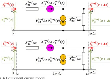
D. An equivalent circuit model
Therefore, we have proven that a set of two wires above an infinite PEC ground plane can be split into two coupled subsets: an internal and an external subset. These may be synthesized in the form of equivalent circuit model of Fig. 6, for a two-wire transmission line.
Fig. 6.Equivalent circuit model
The internal subset is composed of one wire considered as the internal reference of the other wires, whereas the external subset consists of the wire that is previously considered as the internal reference and the global reference (the infinite PEC ground plane). Besides, the internal subset can be assessed by the classical TLT considering the internal reference wire, and the external one through a full-wave solver or by the METLT.
Thus, this innovative approach is referred to as the embedded double reference transmission line theory (EDRTLT), and in the following its resolution algorithm is described.
IV. ALGORITHM OF CALCULATION OF THE P.U.L. PARAMETERS
In order to resolve the EDRTLT equations, the following steps should be followed
1. Step 1:
Calculate the Green's function of the wire taken as the reference in the presence of the infinite ground plane, using (34) or a full-wave solver
Calculate the Green's functions of all the other wires considering only the wire taken as the reference, using (47) and (48), or (49) and (50) in the case of two wires only.
Assemble all scalar Green's function in the [GDR]matrix.
2. Step 2: calculate the inverse matrix of [GDR]
3. Step 3: calculate the double reference impedance and admittance matrices using(29) and (30) 4. Step 4: calculate the single reference impedance
and admittance matrices using the transformation relations (23)-(28)
5. Step 5: resolve (1) and (2) using a classical TLT
solver
In the following, we show a comparison of the p.u.l. parameters calculated directly in the single reference system with those calculated using the above algorithm, in the case of two lossless wires of the same radius a=0.75 mm, separated by a horizontal distance d12=10mm and at two closer heights
h1=100mm and h2=101.5mm above an infinite PEC ground plane, between 10 MHz and 3 GHz.
Fig. 7. Comparison between the single reference p.u.l. resistances obtained directly from the single reference expressions and from the double reference p.u.l. resistances, through the transformation relations.
Fig. 8. Comparison between the single reference p.u.l. inductances obtained directly from the single reference expressions and from the double reference p.u.l. inductances, through the transformation relations.
These p.u.l. parameters are obtained using the transformation relations (23)-(28) that can be considered as another way round to retrieve the single reference parameters from the double reference ones. It is shown in Figs. 7 to 10 that the single reference parameters may be calculated from the double reference ones with a satisfactory accuracy over the entire frequency band for which the ratio h/ ranges from 0 to 1. The remaining differences are due to the approximations (42), (43), (45) and (46) which enable to consider the p.u.l.
parameters of the internal subset as classical ones.
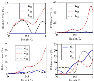
Therefore the main limitation of EDRTLT is related to the approximation of classical p.u.l. parameters for the inner transmission line. In particular, the higher the frequency, the less valid is the approximation of (46). In relation to this, the smaller the distance between wires, the better is the quality of the approximation (46). Fig. 11 provides relative errors of EDRTLT p.u.l. parameters with respect to that of METLT as a function of h/. These relative errors do not increase monotonously but tend to be higher for h/ approaching 1.
Fig. 9. Comparison between the single reference p.u.l. capacitances obtained directly from the single reference expressions and from the double reference p.u.l. capacitances, through the transformation relations.
Fig. 10. Comparison between the single reference p.u.l. conductances obtained directly from the single reference expressions and from the double reference p.u.l. conductances, through the transformation relations.
Fig. 11. Relative errors (%) of EDRTLT p.u.l. parameters with respect to the single reference p.u.l. parameters of METLT (h1=100 mm).
V. VALIDATION
In order to validate the embedded double reference transmission line theory (EDRTLT), some simulations with the METLT (single reference) are carried out.
A circuit composed of two wires of the same geometrical and electrical characteristics is studied (Fig. 12). Each wire is considered as a perfect electrical conductor, of radius a=0.75 mm and length L=1 m. They are located at two different but almost identical heights h1=100mm and h2=101.5mm above an infinite PEC ground plane. The separation distance between the two wires is taken d12=10mm. The time-harmonic voltage
source of 0.632 V is located at z=L of the wire 1, all the loads are of 50 Ω and the analysis is carried out in the 10 MHz to 1 GHz frequency range.
Fig. 12.A two-wire transmission line with excitation source and load impedances definition
The results obtained by the EDRTLT are compared to those obtained through the modified enhanced transmission line theory (METLT). Note that in the METLT as well as in the EDRTLT, the lines are lengthened by their heights.
Figs.13-15 show a good agreement between the single reference results obtained by the METLT and the double reference ones obtained by EDRTLT. However, there are some differences that can be explained by the simplifications made in the calculation of the p.u.l. parameters when extracted from a double reference formulation in the case of the EDRTLT. Therefore, the EDRTLT can be used instead of the METLT in the case of multi-conductor transmission lines.
Fig. 13.Current magnitude as a function of the frequency at load Z1
Fig. 14.Current magnitude as a function of the frequency at load Z2
Fig. 15.Current magnitude as a function of the frequency at load Z3 The above example was that of a two wire-transmission line, each of the inner and outer transmission lines being reduced to two transmission lines with a unique wire. This simple example does not justify by itself the recourse to a double-reference description but provides an idea of the quality of the classical p.u.l. parameters for the inner transmission line. Then, we apply the EDRTLT for a configuration of a transmission line with five wires over the ground as sketched on Fig. 16. The five lossless wires of the same radius a=0.75 mm, are separated by distancesd12= d25= d23= d45= 1.52 mm,
and their heights over the infinite PEC ground plane are h1=h2 - 1.5=h3 -3=h4 -1.5 =h5 - 1.5=100mm. The length of this transmission line is still one meter. Excitation and load configurations are similar to that of Fig.12. In other words, all additional wires are loaded with 50 Ω resistances.
Fig. 16.Configuration of a five wires transmission line over a PEC ground plane.
The p.u.l. parameters of the EDRTLT are calculated from the algorithm given in section IV as for the previous example. For sake of brevity, we do not show the numerous comparisons of individual p.u.l. parameters but rather give the results of current magnitudes at different wireends (z=L).
Fig. 17.Current magnitude as a function of the frequency at load Z2
Fig. 18.Current magnitude as a function of the frequency on wire 2 at load Z4(far-end crosstalk)
Fig. 19.Current magnitude as a function of the frequency on wire 3 at load Z6(far-end crosstalk)
Curves in Figs. 17-19 enable to conclude that EDRTLT provides a good estimate of currents flowing on the transmission line in comparison to METLT taken as reference. Approximation of classical p.u.l. parameters is therefore acceptable for the inner transmission line. The higher frequency band (above 500 MHz) exhibits a slightly less good comparison at resonance frequencies.
We provide in Fig. 20, a relative error for curves of Figs.13-15. We notice that the relative error increases with the frequency as expected. Besides, at resonance frequencies, it becomes larger because the EDRTLT combines the use of the METLT and classical TLT which is known to have issues at resonance frequencies.
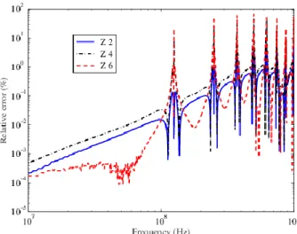
In addition, Fig. 21 gives a summary of relative errors for Figs. 17-19. We notice that the error is smaller in the case of 5 conductors than in the case of 2 conductors. This is due to the fact that, in the former case, the conductors are closer each to another.
Fig. 20.Relative errors (%) between curves of Figs. 13-15.
Fig. 21.Relative errors (%) between curves of Figs. 17-19.
As stated in the introduction and confirmed by the results in Figs 20-21, this approach is rather intended for harnesses that are at a mean height at which the classical TLT is no longer available but still not large enough to use the METLT or MoM approaches. This is confirmed by Fig. 21 that shows that the results have a relative error of less than 1% except at the resonance frequencies at which the EDRTLT inherits the weaknesses of the classical TLT.
VI. CONCLUSIONS
In this paper, a new approach dealing with multi-conductor transmission lines is presented and called embedded double-reference transmission line theory (EDRTLT).
This approach is based upon choosing an arbitrary wire among the wires constituting the harness considering it as a local return conductor. Thus, the p.u.l. parameters of the
N-1remaining wires are calculated with respect to this local
reference. Those p.u.l. parameters are therefore intrinsic to the bundle without any reference to the surrounding ground plane or structure. This internal subset of transmission line system is coupled to an external transmission line with the former local reference taken a single conductor transmission line and the ground plane or structure as a return path for the current.
The transformation from a double to a single reference system is possible and the p.u.l. parameters expressed in the former one can be recast to calculate the parameters of the embedded single reference system. In the case of a bundle of small diameter with respect to its distance over a ground plane, the double-reference p.u.l. parameters may be calculated in a straightforward manner. The p.u.l. parameters of the internal subset may be calculated from the classical quasi-static approximation of the Green’s functions. Thep.u.l. parameters associated to the local reference wire over the ground plane can be calculated using either the METLT p.u.l. parameters if the surrounding structure is simple, or through an exact resolution of Maxwell’s equations in more general situations. Any change of geometry of the transmission line, given the bundle’s diameter remains much smaller than its distance to the grounding structure, requires the only calculation of the p.u.l. parameters of a single wire: This is one of the major advantages of the proposed EDRTLT.
A two-wire transmission line was evaluated for purpose of validation in a direct manner (METLT with a single reference) and through the EDRTLT. Results obtained by this new theory are comparable to those obtained through the METLT. Retrieval of single reference parameter from the double-reference system is indeed effective and may be very useful to simplify the numerical analysis of the bundle to ground interaction.
Many of the figures in this article provide a comparison between single reference and double reference data (Fig. 7-9, 13-15and 17-19). The readers who would like to perform their own analysis of the quality of the comparisons (e.g. using the feature selective validation method in [12]) may find all corresponding data in supplementary files associated with this paper.
ACKNOWLEDGMENT
This work was sponsored by the French C.N.R.S and Groupe PSA.
REFERENCES
[1] A. K. Agrawal, H. J. Price, and S. H. Gurbaxani, “Transient response of multiconductor transmission lines excited by a nonuniform electromagnetic field,” in
Antennas and Propagation Society International Symposium, 1980, 1980, vol. 18, pp. 432–435.
[2] F. Rachidi and S. Tkachenko, Electromagnetic Field
Interaction with Transmission Lines: From Classical Theory to HF Radiation Effects. WIT Press, 2008.
[3] S. Tkatchenko, F. Rachidi, and M. Ianoz, “Electromagnetic field coupling to a line of finite length: theory and fast iterative solutions in frequency and time domains,” IEEE Trans. Electromagn. Compat., vol. 37, no. 4, pp. 509–518, 1995.
[4] Y. Bayram and J. L. Volakis, “A Hybrid
Electromagnetic-Circuit Method for Electromagnetic Interference Onto Mass Wires,” IEEE Trans.
Electromagn. Compat., vol. 49, no. 4, pp. 893–900,
2007.
[5] J. Nitsch, F. Gronwald, and G. Wollenberg, Radiating
non-uniform transmission line systems and the partial element equivalent circuit method. Hoboken, NJ: J.
Wiley, 2009.
[6] A. Maffucci, G. Miano, and F. Villone, “An enhanced transmission line model for conducting wires,” IEEE
Trans. Electromagn. Compat., vol. 46, no. 4, pp. 512–
528, Nov. 2004.
[7] J. B. Nitsch and S. V. Tkachenko, “Complex-valued transmission-line parameters and their relation to the radiation resistance,” IEEE Trans. Electromagn.
Compat., vol. 46, no. 3, pp. 477–487, 2004.
[8] S. Chabane, P. Besnier, and M. Klingler, “Extension of the Transmission Line Theory Application with
Modified Enhanced Per-Unit-Length Parameters,” Prog.
Electromagn. Res., vol. 32, 2013.
[9] S. Chabane, P. Besnier, and M. Klingler, “Enhanced Transmission Line Theory: Frequency-Dependent Line Parameters And Their Insertion in a Classical
Transmission Line Equation Solver,” in Proceedings of
the 2013 International Symposium on Electromagnetic Compatibility (EMC Europe 2013), 2013, pp. 326–331.
[10] S. Chabane, P. Besnier, and M. Klingler, “A Modified Enhanced Transmission Line Theory Applied to Multiconductor Transmission Lines,” IEEE Trans.
Electromagn. Compat., vol. 59, no. 2, pp. 518–528,
2017
[11] C. R. Paul, Analysis of Multiconductor Transmission
Lines. Wiley, 1994
[12] IEEE Standard P1597, Standard for Validation of Computational Electromagnetics Computer Modeling and Simulation – Part 1, 2 2008.