HAL Id: insu-02919773
https://hal-insu.archives-ouvertes.fr/insu-02919773
Submitted on 29 Mar 2021
HAL is a multi-disciplinary open access
archive for the deposit and dissemination of
sci-entific research documents, whether they are
pub-lished or not. The documents may come from
teaching and research institutions in France or
abroad, or from public or private research centers.
L’archive ouverte pluridisciplinaire HAL, est
destinée au dépôt et à la diffusion de documents
scientifiques de niveau recherche, publiés ou non,
émanant des établissements d’enseignement et de
recherche français ou étrangers, des laboratoires
publics ou privés.
Chiara Civiero, John Armitage, Saskia Goes, James Hammond
To cite this version:
Chiara Civiero, John Armitage, Saskia Goes, James Hammond. The Seismic Signature of
Upper-Mantle Plumes: Application to the Northern East African Rift. Geochemistry, Geophysics,
Geosys-tems, AGU and the Geochemical Society, 2019, 20 (12), pp.6106-6122. �10.1029/2019GC008636�.
�insu-02919773�
Chiara Civiero1, John J. Armitage2, Saskia Goes3, and James O. S. Hammond4
1Dublin Institute for Advanced Studies (DIAS), Dublin, Ireland,2Institut de Physique du Globe, Université de Paris,
Paris, France,3Department of Earth Science and Engineering, Imperial College London, London, UK,4Department of Earth and Planetary Sciences, Birkbeck, University of London, London, UK
Abstract
Several seismic and numerical studies proposed that below some hotspots upper-mantle plumelets rise from a thermal boundary layer below 660 km depth, fed by a deeper plume source. We recently found tomographic evidence of multiple upper-mantle upwellings, spaced by several 100 km, rising through the transition zone below the northern East African Rift. To better test this interpretation, we run 3-D numerical simulations of mantle convection for Newtonian and non-Newtonian rheologies, for both thermal instabilities rising from a lower boundary layer, and the destabilization of a thermal anomaly placed at the base of the box (700–800 km depth). The thermal structures are converted to seismicvelocities using a thermodynamic approach. Resolution tests are then conducted for the same P and S data distribution and inversion parameters as our traveltime tomography. The Rayleigh Taylor models predict simultaneous plumelets in different stages of evolution rising from a hot layer located below the transition zone, resulting in seismic structure that looks more complex than the simple vertical cylinders that are often anticipated. From the wide selection of models tested, we find that the destabilization of a 200◦C, 100 km thick thermal anomaly with a non-Newtonian rheology, most closely matches the magnitude and the spatial and temporal distribution of the anomalies below the rift. Finally, we find that for reasonable upper-mantle viscosities, the synthetic plume structures are similar in scale and shape to the actual low-velocity anomalies, providing further support for the existence of upper-mantle plumelets below the northern East African Rift.
1. Introduction
Volcanic rifting is undoubtedly related to the thermal state of the mantle during extension and decompres-sion melting (e.g., White & McKenzie, 1989), and the thermal state of the mantle can be estimated from seismic wave speeds derived from inverse models. The East African Rift (EAR) is the largest active volcanic rift zone on the planet. However, despite the clear evidence for decompression melting, there have been con-flicting interpretations of the thermal state of the mantle below Afar and the Main Ethiopian Rift (MER). Low seismic velocities in the shallow mantle below the rift obtained from surface-wave inversion require a hotter than average mantle of 1450◦C or roughly 100◦C hotter than normal mantle (Armitage et al., 2015). This estimate is consistent with the lower bound of the thermal range 100–200◦C derived from the tomo-graphic velocity models in Civiero et al. (2015, 2016), receiver function estimates (50–100◦C) of Rychert et al. (2012), and analyses of primitve magmas, which suggest low thermal excess for mantle today (Ferguson et al., 2013; Rooney et al., 2012).
Interpretations of inverse seismic velocity models, such as the presence of melt, the shape of the rising plume, or the location of the upwelling source, are rarely tested quantitatively. Older tomographic models for Africa suggested that a broad low-velocity layer was present throughout the whole upper mantle beneath the EAR, interpreted as a large-scale upwelling named the African Superplume (Benoit et al., 2006; Hansen et al., 2012; Ritsema et al., 1999). However, as data and resolution have improved, this structure has been shown to be made up of smaller-scale features (e.g., Chang & Van der Lee, 2011; Emry et al., 2019; Hammond et al., 2013). The body-wave tomographic models of Civiero et al. (2015, 2016) found that the seismic veloc-ity structure below the northern EAR is complex in shape and scale. However, the EAR is not unique in terms of complexity. Recent tomographic studies found evidence of plume branching (Rickers et al., 2016) or, based on the complexity of the imaged seismic structure, proposed the existence of secondary small-scale upper-mantle plumes, or plumelets, rising from a larger thermal anomaly in the lower mantle
Key Points:
• Multiple upper-mantle upwellings rise as Rayleigh Taylor instabilities at different evolutionary stages below Afar and Main Ethiopian Rift • A 200◦C excess temperature source
layer near the top of the lower mantle explains the upper-mantle structure below the East African Rift • Hotspot volcanic centers spaced by
few hundred km are likely fed by hot material which has stagnated at the base of the transition zone
Supporting Information: • Supporting Information S1 Correspondence to: C. Civiero, cciviero@cp.dias.ie Citation:
Civiero, C., Armitage, J. J., Goes, S., & Hammond, J. O. S. (2019). The seismic signature of upper-mantle plumes: application to the northern east african rift. Geochemistry,
Geophysics, Geosystems, 20
Received 23 AUG 2019 Accepted 4 DEC 2019
Accepted article online 6 DEC 2019
©2019. American Geophysical Union. All Rights Reserved.
Published online20DEC2019 , –
6106 6122.https://doi.org/10.1029/ 2019GC008636
Corrected 14 AUG 2020
This article was corrected on 14 AUG 2020. See the end of the full text for details.
(Civiero et al., 2018; Saki et al., 2015). Such a scenario is appealing given that secondary plumes have been shown to occur within laboratory experiments (e.g., Davaille & Vatteville, 2005; Kumagai et al., 2007); however, the hypothesis that follows from the interpretation of seismic tomographic models needs to be numerically tested.
Only a few previous studies have tested the tomographic results against dynamic models to understand the nature of mantle plumes, with very few using resolution tests. Boschi et al. (2007) and Styles et al. (2011) did a comparison of global and regional plume models against global tomography to get an overview of how many plumes might exist. Davaille et al. (2005) looked over a large region encompassing the African and sur-rounding hotspots below the Atlantic and Indian Oceans and qualitatively compared plume styles predicted from analog models. Structures from dynamic plume models have been used by Hwang et al. (2011) and Maguire et al. (2016) to illustrate how wavefront healing may mask the traveltime signatures of plumes below 1,000 km depth. A more recent study of Maguire et al. (2018) carried out synthetic tomography experiments to understand plume resolution given the limitations of network design. Ballmer et al. (2013) performed a regional study focusing on Hawaii and found that numerical models of a complex thermochemical plume are compatible with the tomographic images of the upper mantle below the islands.
In this study, we explore if plumelets are consistent with seismic observations focusing our analysis on the northern EAR. We develop a workflow to model physically plausible plumelet scenarios based on regional mantle flow. We first analyze plume scales and strength in the numerical models as a function of Rayleigh number and temperature contrast across the hot thermal boundary layer. These physical structures are then converted to seismic structures using thermodynamic methods that account for the effects of temperature, pressure, phase, composition, and anelasticity (Cobden et al., 2008; Goes et al., 2004; Styles et al., 2011). We then use these seismic structures as input for synthetic resolution tests using the same data distribu-tion and inversion scheme and parameters as in Civiero et al., 2015 (2015, 2016). Finally, we compare the simulated convective instabilities with the tomography from our seismic observations. This allows us to test the hypothesis that the apparent complexity in seismic tomographic images is due to multiple plume-like structures at distinct stages of evolution within the upper mantle.
1.1. Tomography on the Northern EAR
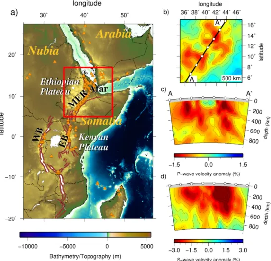
The P and S wave tomography performed by Civiero et al. (2015, 2016) imaged the mantle structure below the northern EAR using seismic stations deployed along the rift (Figure 1). The study region comprises Afar and the MER. This area is characterized by a topographic swell (the Ethiopian Plateau), 30 Myr old flood basalts, and currently active volcanism and extensional faulting (Figure 1a). Seismic stations that were used are from 26 different temporary and permanent arrays that span the region from Saudi Arabia to Madagascar (supporting information Figure S1). This wide aperture allows for high resolution (100–200 km) from 50 km below the study area in the box in Figure 1a down to between 700 and 800 km depth.
Civiero et al. (2015, 2016) applied teleseismic traveltime tomography using the method of VanDecar et al. (1995), on a data set of 16,420 relative P traveltimes and 16,569 relative S and SKS traveltimes. The tomographic models were obtained with regularization parameters that provide a balance between misfit reduction and not overfitting the data beyond the data error estimates (using flattening = 4,800, smoothing = 153,600). We will refer to the P wave model as NEAR-P15 and the S/SKS-wave model as NEAR-S16.
As illustrated in Figures 1b–1d, the tomographic inversion recovered two clusters of low-velocity anomalies, below Afar and MER, that extend from about 200 km depth to the topmost lower mantle. The models clearly illustrate that the two clusters are separate features and are required to extend through the transition zone. The sublithospheric low velocities have been attributed to the spreading of plume material below the litho-sphere, with local contributions from melt (Civiero et al., 2015, 2016). The deeper structures (300–660 km depth) were interpreted as plume tails. Below 700 km depth, the structure changes and appears different in the P and S wave models, in particular below the Afar where the NEAR-S16 shows a high-velocity anomaly while the NEAR-P15 images a low-velocity feature. This is due to the fact that in the topmost lower mantle, the resolving power is weak, especially in the S wave tomography where the resolution does not extend as deep as in the P wave model.
Figure 1. Study area and tomography. (a) The East African Rift region comprising the Afar region, the Main Ethiopian
Rift (MER), and eastern and western branches (EB, WB) south of the study area (red box). Orange triangles represent Holocene volcanoes. Brown lines delineate active fault zones. Stations used were distributed all across the area shown (see Figure S1 for station locations), providing good resolution in the study area within the red box. (b) Horizontal slice at 500 km depth through the undamped P model, NEAR-P15. The black line indicates the orientation of the cross sections in (c) and (d). (c) Vertical cross section through the undamped NEAR-P15. (d) Vertical cross section through the undamped NEAR-S16. The cross section reveals two clusters of low-velocity anomalies below Afar and MER extending down to the base of the transition zone.
1.2. Constraints on Plume Spacing
Various studies have suggested that hotspot or volcanic clusters may share the same root zone. Kumagai et al. (2007) proposed that the French Polynesian hotspots (Tahiti-Macdonald-Pitcairn), the Canaries-Cape Verde-Azores-Great Meteor hotspots, and the Marion-Crozet hotspots share a source comprising ponded material below the 660 km depth seismic discontinuity. Saki et al. (2015), based on the analysis of transition-zone discontinuity topography from PP/SS precursors, proposed that the Canaries-Cape Verde and Azores share a source layer below the transition zone. The recent tomographic models of Civiero et al. (2018, 2019) also suggested that the source of the Canaries' upwelling is a deep Central Atlantic plume region. Tomographic images by Rickers et al. (2016) indicate that Iceland and Jan Mayen are two branches of a common plume below 1,300 km. In all these cases, the spacing between hotspots is around 1,000–1,500 km. Chang and Van der Lee (2011) imaged possible plume conduits below Afar, Kenya, and Saudi Arabia that are separate down to at least 1,500 km depth. Again, spacing between these proposed plumes is about 1,500 km. Other examples suggest a plume spacing of hundreds of km. These include our inferred Afar and MER plumelets, which are separated by 400–600 km (Civiero et al., 2015, 2016), and the proposed baby plumes (Eifel, Massif Central, Bohemian Massif, upper Rhine Graben, and Brest Graben) below Europe (Goes
et al., 1999; Granet et al., 1995)), which are spaced 250–400 km apart. Furthermore, spacing between active volcanoes within the Canaries, Cape Verde, and Society Islands is between 50 and 300 km.
1.3. Dynamic Controls on Plume Spacing
The spacing of thermal plumes that form naturally in laboratory experiments of Rayleigh Bénard convection, where the strongly temperature-dependent viscous fluid is heated from the base and cooled from the top, is a function of the aspect ratio of the rectangular tank and the local Rayleigh number (Androvandi et al., 2011). For fluids that have a viscosity that is an exponential function of temperature, the wavelength, or plume spacing, is observed to decrease with Ra as𝜆∕H ∝ Ra1/3, where H is the height of the experimental tank (Androvandi et al., 2011). In numerical experiments, where the fluid is assumed to be isoviscous, the reduction in wavelength takes the form𝜆∕H ∝ Ra1/6(Galsa & Lenkey, 2007; Zhong, 2005). If we assume that
the plumes initiate at ∼1,000 km depth, then the spacing of the plumes would be of the order of 1,000 km or less, for a local Ra > 105(Androvandi et al., 2011). Therefore, it follows that if the stagnation of large
mantle plumes at shallow depth leads to the formation of plumelets due to the increased temperature at the boundary (e.g., Kumagai et al., 2007), then the spacing will be a function of the depth at which the stagnation occurs.
For the destabilization of a layer of hot material or the development of Rayleigh Taylor instabilities, the growth of the instability should be largest for the characteristic wavelength defined by the aspect ratio of the domain. From linear scaling analysis of the destabilization of a layer equal to one tenth of the height of the region, H, the characteristic wavelength is𝜆 = 0.37H (Schmeling, 1987). This calculation is for two materials of the same viscosity. It was subsequently demonstrated that in 2-D systems, the final dominant wavelength is not necessarily equal to the characteristic wavelength if there was an initial perturbation to the system (Schmeling, 1987). That aside, if we assume a thin layer 100 km thick of hot mantle material ponds at the 660 km depth discontinuity, then the characteristic wavelength of the plumelets would be on the order of 200 km. Given the impact of the initial configuration on the estimate of plume wavelength, we will numer-ically model both Rayleigh Bénard and Rayleigh Taylor instabilities for Newtonian and non-Newtonian rheologies.
2. Dynamic Models Methods
2.1. Numerical Models Setup
We jointly solve the Stokes and energy equations using the numerical code Stag3D (Tackley, 1998) for the flow of a highly viscous fluid within a Cartesian domain of aspect ratios 3 × 3 × 1, 4 × 4 × 1, and 6 × 6 × 1, and the model is 700 or 800 km deep. Mechanical boundary conditions are free slip on all sides and of fixed temperature at the top and bottom. Temperatures are fixed at the top and bottom, and the sides are insulating. Tracers are used to make material at the top—between 0 and 0.14H depth—buoyant, by assigning them a buoyancy number, B, which equals the thermal over chemical density anomaly: B = Δ𝜌c∕Δ𝜌T=0.5 (Fourel,
2009). This depth range will comprise most of the upper thermal boundary layer that forms as the model evolves. This minimizes lithospheric participation in the convection pattern and allows us to focus on plume scales and geometry.
Temperature in the asthenosphere is initially set to 1350◦C, the assumed background mantle potential tem-perature (Armitage et al., 2015). At between 0 and 100 km depth, temtem-perature increases linearly from 0 to 1350◦C. At the bottom of the model, we explore two setups:
• A hot lower boundary condition of 1350◦C + ΔTe, where ΔTeis the excess temperature.
• A basal hot layer, 100 km thick, of excess temperature ΔTeis included in the initial condition, and the lower boundary temperature is held at 1350◦C.
The former lower boundary condition will lead to Rayleigh Bénard convection, while the latter initial condition will destabilize in the form of Rayleigh Taylor instabilities.
The form of the convective instabilities will be determined by the rheology of the upper mantle. We test two different dominant mechanisms for mantle creep, diffusion, and dislocation creep, which can be expressed as a Newtonian and a non-Newtonian rheology. The first rheology we take is an idealized temperature-dependent Newtonian material written as
𝜂 = 𝜂0Arefexp
( E
RT
)
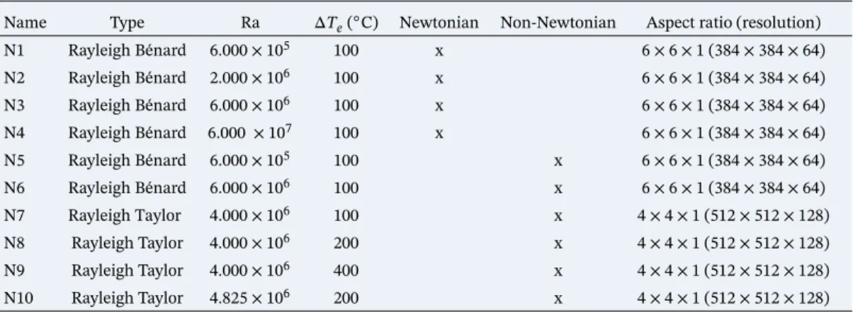
Table 1
List of Models
Name Type Ra ΔTe(◦C) Newtonian Non-Newtonian Aspect ratio (resolution)
N1 Rayleigh Bénard 6.000×10⁵ 100 x 6×6×1 (384×384×64) N2 Rayleigh Bénard 2.000×10⁶ 100 x 6×6×1 (384×384×64) N3 Rayleigh Bénard 6.000×10⁶ 100 x 6×6×1 (384×384×64) N4 Rayleigh Bénard 6.000 ×10⁷ 100 x 6×6×1 (384×384×64) N5 Rayleigh Bénard 6.000×10⁵ 100 x 6×6×1 (384×384×64) N6 Rayleigh Bénard 6.000×10⁶ 100 x 6×6×1 (384×384×64) N7 Rayleigh Taylor 4.000×10⁶ 100 x 4×4×1 (512×512×128) N8 Rayleigh Taylor 4.000×10⁶ 200 x 4×4×1 (512×512×128) N9 Rayleigh Taylor 4.000×10⁶ 400 x 4×4×1 (512×512×128) N10 Rayleigh Taylor 4.825×10⁶ 200 x 4×4×1 (512×512×128)
where𝜂0is the scaling viscosity, Aref=2.2×10⁻⁵ is the prefactor, E = 120 kJ mol−1is the activation energy,
R = 8.31 is the ideal gas constant, and T is mantle potential temperature. The activation energy, which was determined empirically for the upper mantle to achieve agreement between calculations and observa-tions of lithosphere plate flexure, is a factor of 3 lower than experimentally derived estimates (Korenaga & Karato, 2008; Watts & Zhong, 2000). However, as shown by Christensen (1984) and Jaupart and Mareschal (2011), a small value for the activation energy may be regarded as a convenient way to approximate nonlinear diffusion creep with a Newtonian analog.
The second rheology we consider is a strain weakening non-Newtonian temperature and pressure-dependent creep law
𝜂 = 𝜂0A 1 n refexp (E + pV nRT ) . I2 1−n n , (2)
where the prefactor Aref=1.47 × 10⁻¹⁶for a reference strain rate of 10−15s−1, E = 523 kJ mol−1, activation
volume V = 4 cm3mol−1, stress exponent n = 3.6 (Korenaga & Karato, 2008), andI.
2is the second invariant of
the deviatoric strain rate tensor. Finally, in both models, the scaling viscosity,𝜂0, is set by the initial Rayleigh
number
Ra = 𝛼g𝜌mΔTH
3
𝜅𝜂0
, (3)
where H is the height of the model domain and𝛥T = 1350◦C. The remaining constants are listed in Table S1. We explore initial Ra of 105to 107. The various models are listed in Table 1.
3. Dynamic Models—Plume Scales and Styles
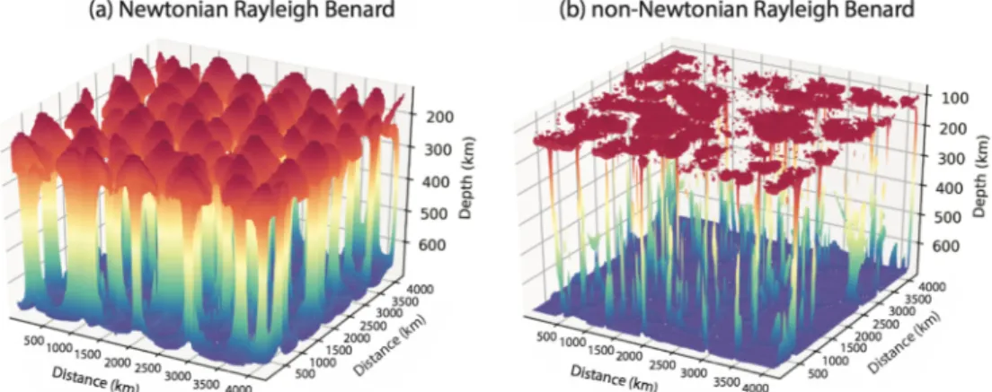
For the Rayleigh Bénard experiments, the model generates regularly spaced plumes for both the Newto-nian and non-NewtoNewto-nian rheologies (Figure 2). These plumes grow uniformly across the model domain, and the spacing is a function of the initial Ra (Figure S2). For the temperature-dependent Newtonian rheol-ogy (Models N1 to N4; Table 1), rather, classic mushroom-shaped plumes are generated (Figure 2a). These plumes eventually impinge on the buoyant lithosphere. The non-Newtonian model plumes (Models N5 and N6; Table 1) are significantly thinner, with plume heads that rapidly flatten out under the lithosphere (Figure 2b). Using the definition of Labrosse (2002) for finding the plume wavelength, we search for the distance between temperature anomalies of
T> ̄T + 𝑓(Tmax−Tmin
)
, (4)
where ̄Tis the mean temperature, Tmaxis maximum temperature, Tminis the minimum temperature, and
f = 0.2. As in previous studies, we find that the wavelength of the plumes is a function of the Ra number (Androvandi et al., 2011; Galsa & Lenkey, 2007; Zhong, 2005). The trend in reduction in wavelength fol-lows𝜆∕H ∝ Ra1/6; however, given the range in measured wavelengths, we cannot rule out the possibility
that𝜆∕H ∝ Ra1/3, as found for laboratory experiments using fluids with a strongly temperature-dependent
Figure 2. Surface plots of the 1% thermal anomaly (corresponding to a temperature of 1363.5◦C) colored by depth. The models represent Models N3 and N6 in Table 1 and have the same Ra=6 × 10⁶. (a) Rayleigh Bénard convection for a
Newtonian rheology showing equally spaced plumes that developed uniformly in time. (b) Rayleigh Bénard convection for a non-Newtonian rheology. In this case the strain rate dependence creates thin plumes with flat heads that rapidly impinge on the lithosphere. Note that the aspect ratio is distorted.
(Models N5 and N6) would suggest a stronger dependence of wavelength on Ra when compared to the Newtonian models (Figure S2b).
If we scale the dimensionless wavelength by the depth to the 660 km depth discontinuity, we find that the possible EAR plumelets could be explained by Newtonian plumes with an upper mantle of Ra > 106
(Figure S2a). This corresponds to a scaling viscosity,𝜂0 < 5 × 10²⁰Pa s. For non-Newtonian plumes, the
wavelength of EAR plumelets corresponds to a Ra for the upper mantle of ∼ 106or a reference viscosity of
𝜂0< 5 × 10²⁰Pa s. However, these plumes are very likely too thin to be seismically visible.
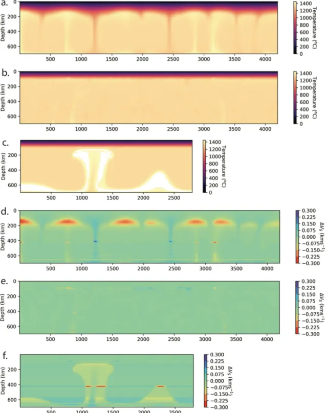
The Rayleigh Bénard convection develops uniformly. The Rayleigh Taylor destabilization of a hot layer of material is however not uniform in time. In Figure S3, we show two models with different aspect ratios, 3 × 3 × 1 and 4 × 4 × 1, respectively, where early- to late-stage plume (LS)-like structures can be detected within the same snapshot. The spacing of these instabilities is of the order𝜆 = 0.5H to 𝜆 = H depend-ing on the aspect ratio of the model domain and the stage at which the plume forms (Figure S3). The first instability always forms at a corner of the model, and this subsequently leads to a destabilization of the hot layer that propagates outward from the corner. The wavelength of the plume-like structures was found to be independent of the temperature of the hot layer, as this did not significantly affect the initial Ra number. Fur-thermore, the contrast in temperature is high for these plumes when compared to the Newtonian Rayleigh Bénard convection (Figures 3a–3c). This high contrast is due to the non-Newtonian rheology, which leads to a sharper viscosity contrast between the cold and hot material, therefore keeping the sharp thermal gradient. The strong temperature contrast is thus important in the experiments.
When calculated seismic structures are converted to synthetic tomography, the inverted magnitude of VSor
VPdiminishes (e.g., Goes et al., 2012; Maguire et al., 2018). Therefore, a strong temperature contrast might be
required to match the significantly low seismic velocities observed below Afar and the MER (Figures 1b–1d). This would suggest that the Rayleigh Taylor structures would more likely correspond to the observed tomog-raphy. The wavelength of the plumelet spacing is however in this case dependent on the model aspect ratio. For Models N7 through to N9, the spacing is closer to 1,000 km as shown in Figure S3. Given that the Rayleigh Taylor plumelets can (i) match the observed spacing, (ii) have a stronger temperature contrast, and (iii) gen-erate instabilities at different stages of evolution, we will explore how they are transformed when viewed as seismic anomalies.
4. Synthetic Tomography Methods
4.1. Conversion to Seismic Anomalies
To convert the thermal plume structures into velocities and density, we follow the approach of Cobden et al. (2008) and Styles et al. (2011). We use the thermodynamic code PerPlex (Connolly, 2005) with the NCFMAS data base “stx08” (Xu et al., 2008) to calculate the elastic parameters (bulk modulus K and shear modulus G) and density as a function of pressure, temperature, and composition. For the basic conversions,
Figure 3. (a–c) Cross sections through the Newtonian Rayleigh Bénard Model N3 (a), the non-Newtonian Rayleigh Bénard Model N6 (b), and the
non-Newtonian Rayleigh Taylor Model N7 (c) illustrating the potential temperature in◦C. Note the stronger temperature contrast for the Rayleigh Taylor Model N7. (d–f) Cross sections of the S wave seismic velocity anomaly (in km/s) relative to the reference velocity taken from an unperturbed region for the Newtonian Rayleigh Bénard Model N3 (d), the non-Newtonian Rayleigh Bénard Model N6 (e), and the non-Newtonian Rayleigh Taylor Model N7 (f). Note that the anomaly range on (e) is smaller than on (d) and (f).
we assume a pyrolite composition, except for the continental lithosphere which is taken to be harzburgitic (both compositions from Xu et al., 2008). A constant adiabatic temperature gradient of 0.45 K km−1(a
rea-sonable upper-mantle average, according to Styles et al., 2011) is added to the potential temperatures from the Boussinesq model. The velocities have further been corrected for the effects of temperature, pressure, and hydration-dependent anelasticity using composite model Qg(Goes et al., 2012; van Wijk et al., 2008) for a frequency of 1 Hz (which is good for the P waves but on the high side for the S waves). The mantle is assumed to contain a slight amount of water as estimated for the MORB-source (1,000 H/Si), and the conti-nental lithosphere is dry (50 H/Si) (Goes et al., 2012). Anomalies are calculated relative to a part of the model without plumelets and where the boundary layers are least perturbed. We subtract our synthetic reference model from the 3-D synthetic velocities as our inversion is not sensitive to the reference model (Cammarano et al., 2005). The uncertainties involved in the calculation of elastic and anelastic parameters lead to uncer-tainties in VPand VSanomalies of around ±0.1% and ±0.15%, respectively (Cammarano et al., 2003; Styles
et al., 2011).
The plumelets can be seen in the seismic velocity anomalies to varying degrees depending on the model rheology and if they are due to Rayleigh Bénard convection (Models N1 to N6; Figures 3d and 3e) or if they form due to the destabilization of a hot layer (Models N7 to N10; Figure 3f).
4.2. Tomographic Method
We test how the synthetic structure is imaged using the tomographic relative traveltime inversion for P and
Swave velocity following the method of VanDecar et al. (1995). This technique retrieves velocity anoma-lies relative to the average regional background. We perform a linear inversion and use ray theory, which leaves some uncertainties in the determination of the magnitude of the velocity anomaly, but should not change the overall anomaly patterns with depth (Montelli et al., 2004). We calculate the arrival times by applying full 3-D ray tracing (Julian & Gubbins, 1977) through the synthetic models and add Gaussian random noise to the synthetic data, respectively, 0.07 and 0.37 s for P and S wave data, that is, of similar magnitude as the estimated errors in the real data. We invert for these synthetic velocity structures using the same model parameterization, regularization parameters, and raypaths (calculated through the iasp91 1-D velocity model) as used in the tomography models of Civiero et al. (2016, 2015).
The resolution in the shallow upper mantle (0–200 km depth) is low due to a lack of crossing rays at this depth range. In the inversion of seismic observations (Civiero et al., 2016, 2015), we investigated both models that were solely constrained by the traveltimes, as well as models where the 3-D structure obtained from the surface-wave model of Fishwick (2010) was imposed as a starting model that the inversion was damped to, as an additional constraint on the shallow mantle structure (see Civiero et al., 2015, for further details). Without adding an a priori constraint on shallow structure, horizontally extensive anomalies, such as the high-velocity lid and low-velocity plume material spread below it, are poorly resolved, but the traveltimes provide the main constraints on the plumelet tails and lateral variations in structure that reflect plume shapes. We first focus on such undamped cases but then run additional inversions where we mimic the effect of damping in the synthetic tomography, by moderately damping the model (damping = 35) toward the synthetic structure down to 300 km. This is an optimistic test, as surface-wave tomography will not retrieve the exact seismic structure; therefore, the damped version for the observed tomography is likely somewhere between the undamped and damped synthetic cases.
To perform the resolution tests, the numerical models need to be projected onto the tomographic grid. This is done by preserving slowness within each nodal volume. Because the tomographic grid is coarser than the numerical one, some of the finer-scale features are smoothed when the numerical model is resampled onto the tomographic grid. The volume of the whole tomographic model spans the range 28◦N to 25.40◦ S in latitude, 25–57.20◦E in longitude and 0–2,000 km in depth (the black box in Figure S4), with a node spacing, respectively, of 0.5◦, 0.4◦, and 50 km. We focus our interpretation within the region (5–17◦N and 35–47◦E) comprising the Afar and MER regions (blue box in Figure S4, area outlined in Figure 1a), where we have the highest density of crossing rays. The numerical models vary their size depending on the case and extend from the surface up to ∼700–800 km depth (red box in Figure S4 shows the approximate volume that they span). Depending on the features we analyze, we rotate the model to position the different synthetic plume anomalies in the locations of the two main low-velocity anomalies found in the observed P and S wave tomography, below Afar and the MER.
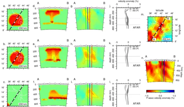
Figure 4. Horizontal slices and vertical cross sections through the P wave Model N7 with a 100◦C hot layer, focused below Afar. The orientation of the cross sections (black line) is shown in each 200 km depth slice. (a–c) Horizontal slices at 200 km depth through the synthetic models of LS (a), MS (b), and ES (c) phases. (d, g) Synthetic and resolved images of the LS plume phase; (e, h) synthetic and resolved images of the MS plume phase; (f, i) synthetic and resolved images of the ES plume phase. (j-l) Input and retrieved P wave velocity anomaly envelopes (%) along the green, blue, and red profiles drawn in the cross sections. (m) The 200 km depth slice through the NEAR-P15 model. (n) Vertical cross section through the NEAR-P15 model. The spacing between the contours is 0.25 %. White points indicate the distance every2◦. The color scale is the same for all the panels.
5. Synthetic Tomography Results
We focus on the Rayleigh Taylor instabilities given that they have a strong temperature contrast (Figure 3) and have widths that are similar to those inferred from the tomographic inversion of the observations. We will first use models with an aspect ratio 4 × 4 × 1 and Ra=4 × 10⁶(Models N7 to N9; Table 1) to test which
plume style and thermal anomaly are required below Afar and the MER to match the seismic observa-tions. Models N7 to N9 have a wide plumelet spacing, due to their large aspect ratio. This large aspect ratio was chosen to achieve the required numerical resolution to solve for the destabilization of a hot layer with temperatures ranging from 100 to 400◦C (Table 1) while efficiently spreading the numerical model across compute nodes. With these models, we will explore how different individual plumelets potentially match the observed tomography in terms of shape and temperature, and we do this by positioning them in turn below Afar and the MER. Next we use the synthetic model with the thermal anomaly that best matches the observed anomalies but with a higher Ra (Model N10) to try to obtain the spacing of the plumelets below the Afar and MER.
5.1. Plume Temperature and Geometry
To test how the different plume geometries corresponding to different stages of plume evolution might be resolved by traveltime tomography, we identify three distinct evolutionary phases from Models N7 to N9 (labeled in Figure S3). The first is an early-stage plume (ES) that is ascending from the thermal bound-ary layer and penetrating into the upper mantle without a well-defined head. The second structure is a middle-stage plume (MS) with one or more thinner feeder columns of ∼150 km diameter and a pronounced blob-like head, which has developed in the upper mantle but has not reached the surface yet. The third is a LS, which shows the classical mushroom-type structure with a head spreading at the base of the lithosphere, fed by a thinner tail.
We then place the ES, MS, and LS plumes in turn below the Afar and MER regions to compare the amplitude of the recovered and actual velocity anomalies for the three models (N7 to N9) having different thermal boundary layers (100, 200, and 400◦C). The velocity amplitudes for the temperature anomaly in Model
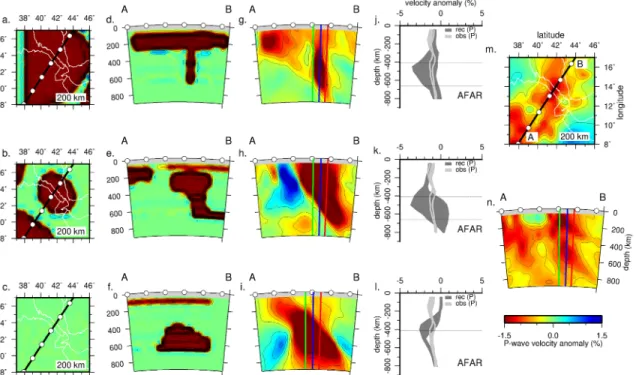
Figure 5. Same as Figure 4 but for the P wave Model N9 with a 400◦C hot layer, focused below Afar.
Figure 6. Horizontal slices and vertical cross sections through the P wave Model N8 with a 200◦C hot layer, focused below Afar. The orientation of the cross sections (black line) is shown in each 200 km depth slice. (a–c) Horizontal slices at 200 km depth through the synthetic models of LS (a), MS (b), and ES (c) phases. (d, g) Synthetic and resolved images of the LS plume phase; (e, h) synthetic and resolved images of the MS plume phase; (f, i) synthetic and resolved images of the ES plume phase. The resolved LS plume (g) lost its head due to the lack of resolution at shallow upper-mantle depths. The MS phase (h) is well resolved because the head of the input model (b) is relatively strong and laterally confined. Although some smearing, the ES structure (i) is quite well recovered. (j–l) Input and retrieved P wave velocity anomaly envelopes (%) along the green, blue, and red profiles drawn in the cross sections. Within the transition zone the retrieved and observed velocity anomalies of the MS and LS plumes overlap. (m) The 200 km depth slice through the NEAR-P15 model. (n) Vertical cross section through the NEAR-P15 model. The spacing between the contours is 0.25 %. White points indicate the distance every2◦. The color scale is the same for all the panels.
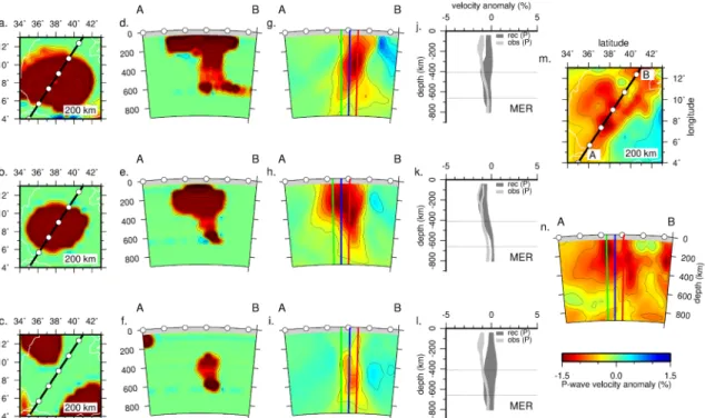
Figure 7. Same as Figure 6 but focused below MER. The LS plume shows the best matching between the retrieved and observed velocity anomalies at
transition-zone depths.
N7 are low relative to the observed structures (Figure 4), and the velocity amplitudes for the temperature anomaly in Model N9 are almost double the observed seismic velocity anomalies (Figure 5). Similar results are obtained for the MER regions and are shown in Figures S5 (Model N7) and S6 (Model N9). Instead, the retrieved plumes in Model N8 correlate quite well with the tomography-imaged features in terms of magnitude (see Figures 6 for Afar and 7 for MER). It would appear therefore that the destabilization of a 200◦C anomaly best matches the velocity magnitudes.
We now explore how the different plume phases LS, MS, and ES are tomographically resolved below the northern EAR. The recovered images for each plume stage are complex and not straightforward to interpret. All the plume stems are resolved through the whole upper mantle; however, without additional constraints on shallow structure, the retrieved image of the LS plume does not resolve the head above 300 km depth, and in absence of smearing, it can be mistaken for a plume in a less evolved phase. The synthetic MS plume image is more distinct from the ES and LS plumes, as the upper-mantle head of the plume is broader and can be resolved laterally (Figures 6 and 7).
The velocity anomalies of both the LS and MS phases overlap in the upper mantle below Afar and are in the range 0.5–1.5% (Figures 6g and 6h) although visually, the MS anomaly is closer to the observed struc-ture in terms of geometry. Below the MER, the LS plume shows the best match between the observed and recovered velocities at transition-zone depths, of around 0.5–1% (Figures 7g and 7h). In turn, the MS phase best matches the elongated shape of the plume. In the uppermost mantle, the imaged velocity anomaly appears more similar to that of the retrieved MS plume (Figure 6h). Note that the tomography below Afar requires significant low-velocity anomalies throughout the depth range of the upper mantle, while below the MER, anomalies in the shallow mantle above 400 km need to be more pronounced than those in the transition zone.
5.2. Plume Scale and Spacing
Figure S7 shows a 3-D perspective plot of the plume model N10 with a destabilization of a 200◦C hot layer, aspect ratio of 4 × 4 × 1, and Ra =4.8 × 10⁶(Table 1). The isosurface of the 1% excess temperature
rela-tive to the surroundings illustrates the number, size, and the morphologies of the upwellings that form. By keeping the same model aspect ratio as Models N7–N9 and slightly increasing Ra, the plumelet spacing is reduced, on the order of 500 km, and this allows us to rotate two plumes into a position that matches the two low seismic anomalies found below Afar and the MER. We rotated the model to place a MS plume
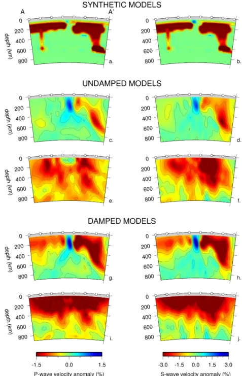
Figure 8. (a, b) Input P (a) and S wave (b) velocity anomalies (%) along a vertical cross section through the Model N10
oriented such that the two plumes are positioned approximately under Afar and MER. The location of the cross sections (black line) is shown in Figure 1b. The structure on the right represents the synthetic MS plume and the structure on the left the LS plume. (c, d, g, h) Vertical cross sections through the recovered undamped P (c) and S wave (d) models and the damped P (g) and S wave (h) models. (e, f, i, j) Vertical cross sections through the undamped (e) and damped (i) NEAR-P15 model and the undamped (f) and damped (j) NEAR-S16 model. The spacing between the contours is 0.25 % for P wave models and 0.50 % for S wave models. The undamped models (c, d) image the tail of the MS plume, but the LS plume recovery is almost completely lost. The damped recovered models (f, g) are able to resolve the MS plume structure and the head of the LS plume but with relatively subdued amplitudes. The scale of the recovered structures is quite similar to that of the imaged features.
with a broad head and a thick stem below Afar and a LS plume with a head spread at the base of the lithosphere and a narrow tail below MER. Synthetic cross sections of the same orientation as the section through Models NEAR-P15 and NEAR-S16 in Figure 1 are shown in Figures 8a and 8b. Model N10 is able to reasonably match both scales and amplitudes of the anomalies in the tomography of the actual data (Figure 8).
In the undamped case, details of the MS plume located below Afar, such as a partially folded head and a tail influenced by phase-boundary topography, are not identifiable in the P wave inversion (Figure 8c). In the S wave model, the head and the tail are slightly better resolved (Figure 8d). The recovery of the plume geometries can be enhanced if constraints on the shallow structure and damping toward it are added (Civiero et al., 2016, 2015). In fact, when considering the damped case, the MS anomaly is generally well recovered in both P and S wave tests (Figures 8g and 8h). The anomaly from the LS upwelling located below the MER is recovered less clearly, where the plume head is almost fully unresolved in both the P wave (Figure 8c) and
Swave models (Figure 8d). Again, when adding constraints on the shallow structure and damping toward it, the recovery of the anomaly improves significantly and better resembles the observed structure below the MER (Figures 8g and 8h). Some of the differences between the recovery of the two plumes may be due to different resolution below Afar and the MER as the data coverage is slightly higher in the first region than in the latter.
Although a Cartesian model of the destabilization of a 200◦C hot layer cannot be expected to match the actual imaged structures in detail, the scale and spacing of the modeled plumes, after accounting for the seismic resolution, is similar to the observed features. Only the low velocities at shallow depths, in particular below the MER, are not as widespread in the synthetic tomography compared to the observed tomography, but the effects of melt retention or local lithospheric thinning, which were not considered, may contribute to these shallow anomalies. The similarity suggests that small upper-mantle plumelets are a plausible expla-nation for the seismic anomalies beneath East Africa, which can also explain the surface expressions of volcanism and rifting.
Interestingly, NEAR-P15 and NEAR-S16 have some differences in relative P wave over S wave anomaly amplitude and structure of the low-velocity anomalies below Afar and the MER (Figures 8e and 8f; Civiero et al., 2016). For example, the tomographic S wave anomaly below Afar in NEAR-S16 is much stronger in amplitude compared to that beneath the MER. This feature is not recovered in the synthetic tomography tests. In addition, some localized strong low-velocity bodies appear in the upper mantle of our tomographic model below the MER. The fact that the differences between synthetic and tomographic amplitudes are more pronounced in S than P wave models could indicate that other nonthermal effects play a role. It has been demonstrated that excess temperatures of around 100◦C may be enough to produce melt volumes below a rift (Armitage et al., 2015). Indeed, a signature of partial melt within the asthenosphere has pre-viously been invoked as additional contribution to the S wave anomalies below Afar (e.g., Bastow et al., 2005; Hammond et al., 2013; Rooney et al., 2012; Thompson et al., 2015). Receiver function studies from Thompson et al. (2015) image a distinct low-velocity zone just on top of the transition zone beneath Afar, which has been interpreted to be a melt layer caused by the release of volatiles from an upwelling. Rooney et al. (2012) also proposed a contribution of deep CO2-assisted melting to the low-velocity features in the asthenosphere below Afar. The presence of melt at the lithospheric depths (<80 km) and/or lithospheric thinning would further enhance shallow low-velocity anomalies (e.g., Rychert et al., 2012; Hammond et al., 2013; Benoit et al., 2006; Kendall et al., 2005). However, the observed dVP∕dVSratios are also affected by differences in spatial resolution for the two data sets, for example, due to the added lateral resolution sup-plied to the S wave velocity inversion by the SKS-wave traveltimes (Civiero et al., 2016). These uncertainties preclude distinguishing thermal from chemical effects with the dVP∕dVSratios from this type of traveltime tomography (Civiero, 2016).
6. Discussion
6.1. Different or Similar Evolutionary Stage Plumes Below Afar and MER
Comparing forward models with observed tomography to find a good match between synthetic and observed features is not straightforward. Tomographic resolution is spatially variable and highly nonlinear, making
it difficult to assess (Rawlinson et al., 2010). However, from our set of resolution tests for each plume stage of evolution, we recognize that models with a strong tail and no head, like ES plumes, do not match our observations well in character or amplitude at upper-mantle depths as both the seismic anomalies below Afar and the MER are much stronger in magnitude (Figures 6 and 7). Generally, plumes in a late phase (LS) and middle phase (MS) of evolution with a broad head and a quite thick tail seem to best explain the evolutionary stage of both the upper-mantle structures below Afar and the MER.
A MS plume below Afar matches well the amplitude of both the P and S wave low-velocity anomalies within the transition zone and above. Moreover, the similarity between the retrieved and observed tomographic plume geometries is encouraging, especially for the S waves (Figure 8). Due to the poorer resolution moving to the SW, identifying the exact stage of evolution of the plume below MER is more difficult. As the observed low-velocity anomaly within the transition zone is narrower compared to that below Afar, we suggest that the plume below MER could be in a slightly more advanced stage, with a head spreading at the base of the lithosphere and a thinner tail. However, the stem of the LS plume shown in Figure 8 is likely too narrow, and a plausible diameter may be closer to that of the LS plume in Figure 7, around 200 km.
The resolution tests also strongly indicate that the source layer of the plumelets lies below 660 km depth but not much deeper. Calculations of the vertical correlation of the NEAR-P15 and NEAR-P16 structures as a function of depth show that correlations are high in the transition zone (>0.6) down to 700 km and decrease strongly below (Civiero, 2016). Similar decreases are found in synthetic tests where the boundary layer is located below this depth, while the decrease in correlation would be significantly more subdued if the boundary layer was located even deeper (e.g., 1,000 km). The dynamic models also indicate that the plume scale and spacing of several hundred km inferred from the seismic images below the EAR is in the range expected for a source layer at the base of the upper mantle and reasonable upper-mantle rheologies. We would therefore suggest that hotspot volcanic centers clustered on the scale of a few hundred km, such as within the Canaries and within western Europe, are likely rooted in hot material that has accumulated just below the transition zone, while the larger spacing of 1,000 1,500 km as imaged for example by Rickers et al. (2016) may be due to the accumulation of hot buoyant material deeper in the lower mantle or plume branching in the lower mantle which occurs in some dynamic models (e.g., Davies & Davies, 2009). 6.2. Secondary Plumes or Destabilization of Ponded Plume Material
We infer that a source layer with a temperature excess of ∼200◦C from a thermal boundary layer is needed to match the amplitude of the upper-mantle low-velocity anomalies imaged in our observed tomography. Yet, it is difficult to reconcile the seismic signatures with a steady-state thermal boundary layer. The Rayleigh Bénard instabilities either are too diffuse (Newtonian Models N1 to N4; Figure S2a) or create anomalies that are too thin (non-Newtonian Models N5 and N6; Figure S2b), such that the thermal anomalies are seismically invisible or relatively weak (e.g., Goes et al., 2004). It is only for the Rayleigh Taylor models (N7 to N10) that thermal anomalies are sufficiently strong such that the seismic velocity anomaly is resolved in the synthetic tomography. Furthermore, only the Rayleigh Taylor models produce simultaneous plumes at different stages of their evolution as may be required by the complexity of the imaged structures.
This is a strong statement, as it implies that the plumelets are more time dependent than secondary instabil-ities that can rise from a regional boundary layer that gradually grows by a deeper plume flux. For example, in models like those by Kumagai et al. (2007, 2008), Tosi and Yuen (2011), and Bossmann and Van Keken (2013), the density contrast between the lower and upper mantle that would be due to the endothermic phase transition can lead to the stagnation of plume material below the boundary. This results in the heating of the boundary between the two layers and the generation of secondary plumes (Kumagai et al., 2007). This process is therefore similar to the Rayleigh Bénard numerical models in Figures 2 and 3, which are either too diffuse or thin to be seismically imaged. Thermal-chemical plumes will stagnate if the compositional buoyancy is such that they become of equal density with the surrounding mantle. The chemical component of the plume will subsequently fall down back into the lower mantle (Kumagai et al., 2008). It is possible that some of the chemical heterogeneity become entrained within the thermal upwellings, but again, these plumes are not the equivalent of the Rayleigh Taylor numerical models that more closely match the seismic observations.
What we require is the arrival of some distinct buoyant material at between 800 and 660 km depth below the EAR. This material would either already be intrinsically unstable or transform to a relatively buoyant mass (e.g., by phase transitions or internal heating) to subsequently spawn the plumelets observed within
the tomographic images. A contribution of chemical heterogeneity to the plume may be required to gen-erate such complex and time-dependent behavior (e.g., Kumagai et al., 2008) and has been proposed to explain the complexity of low-velocity structures in global tomographic images (e.g., Cottaar & Lekic, 2016; Davaille et al., 2005). The scenario of Rayleigh Taylor instabilities could occur if the large-scale thermo-chemical plumes are also internally heated (Fourel et al., 2017). In this case, the large-scale plume rises until it becomes neutrally buoyant. As it stagnates, internal heating will increase its temperature allowing for further destabilization. The tomographic images of the upper mantle are in agreement with relatively fat, thermal anomalies, as in models that include distinct density layers and internal heating (Fourel et al., 2017; Limare et al., 2019).
7. Conclusions
We find that the seismic structure seen in the upper mantle below the EAR is similar in character, scale, and amplitude to predictions from dynamic models for mantle plumelets originating from a 200◦C excess temperature layer near the top of the lower mantle. This suggests that lower-mantle plume material rising upward toward the upper mantle may stabilize in the shallow lower mantle. Subsequently, for example, due to a combination of chemical heterogeneity and internal heating, the structure will destabilize into upper-mantle plumelets with a spacing that is a function of the depth at which the structure stabilizes and its width. Below the EAR, it would appear that African Superplume material accumulated at ∼800 to 660 km depth and subsequently destabilized into several Rayleigh Taylor-style instabilities rising beneath Afar and the MER.
The synthetic tomography generated from the 3-D models of Rayleigh Taylor instabilities highlights that plumes have complex signatures in tomographic images. This suggests that checkerboard tests and sim-ple vertical cylindrical features used as model inputs are insufficient to test interpretations of tomographic images. In particular, if several plumelets are active below a region and they are in different stages of evo-lution, as predicted in our dynamic models, there will be complexities in both geometry and amplitude of the recovered synthetic tomography. This may explain the upper-mantle low-velocity anomalies that differ in shape from simple near-vertical cylindrical structures under a wide number of hotspot regions on scales of several 100 km, for example, in the central Atlantic (Azores, Canaries, Cape Verde, Madeira, and Great Meteor) where an irregularly shaped anomaly of low P wave velocities in the shallowest 200 km, which slants northeast and downward to the top of the transition zone is imaged (Vinnik et al., 2012; Yang et al., 2006), beneath Central Europe where the low-speed anomalies show more than one branch in the upper mantle (Massif Central/Eifel; Granet et al., 1995; Ritter et al., 2001), and Indian Ocean (Marion/Crozet) where several tilted upper-mantle upwellings are suggested to rise from transition-zone depths (Davaille et al., 2005; Montelli et al., 2004). Given that other regions exhibit similarly complex upper-mantle structure and/or spacing between volcanic centers, it would be worthwhile reanalyzing some previously published tomographic images below hotspots in this light.
References
Androvandi, S., Davaille, A., Limare, A., Foucquier, A., & Marais, C. (2011). At least three scales of convection in a mantle with strongly temperature-dependent viscosity. Physics of the Eath and Planetary Interiors, 188, 132–141. https://doi.org/10.1016/j.pepi.2011.07.004 Armitage, J. . J, Ferguson, D. J., Goes, S., Hammond, J. O. S., Calais, E., Rychert, C. A., & Harmon, N. (2015). Upper mantle temperature
and the onset of extension and break-up in Afar, Africa. Earth and Planetary Science Letters, 418, 78–90. https://doi.org/10.1016/j.epsl. 2015.02.039
Ballmer, M. D., Ito, G., Wolf, C. J., & Solomon, S. C. (2013). Double layering of a thermochemical plume in the upper mantle beneath Hawaii. Earth and Planetary Science Letters, 376, 155–164. https://doi.org/10.1016/j.epsl.2013.06.022
Bastow, I. D., Stuart, G. W., Kendall, J. M., & Ebinger, C. J. (2005). Upper-mantle seismic structure in a region of incipient continental breakup: Northern Ethiopian rift. Geophysical Journal International, 162, 479–493. https://doi.org/10.1111/j.1365-246X.2005.02666.x Benoit, M. H., Nyblade, A. A., & VanDecar, J. C. (2006). Upper mantle P-wave speed variations beneath Ethiopia and the origin of the Afar
hotspot. Geology, 34, 329–332. https://doi.org/10.1130/G22281.1
Boschi, L., Becker, T. W., & Steinberger, B. (2007). Mantle plumes: Dynamic models and seismic images. Geochemistry Geophysics
Geosystems, 8, Q10006. https://doi.org/10.1029/2007GC001733
Bossmann, A. B., & Van Keken, P. E. (2013). Dynamics of plumes in a compressible mantle with phase changes: Implications for phase boundary topography. Physics of the Earth and Planetary Interiors, 224, 21–31. https://doi.org/10.1016/j.pepi.2013.09.002
Cammarano, F., Deuss, A., Goes, S., & Giardini, D. (2005). One-dimensional physical reference models for the upper mantle and transi-tion zone: Combining seismic and mineral physics constraints. Journal of Geophysical Research, 110, B01306. https://doi.org/10.1029/ 2004JB003272
Acknowledgments
The authors would like to thank the two reviewers and the Editor, Maureen Long, for constructive, helpful suggestions. C. C. was supported by a Janet Watson Fellowship from the Department of Earth Science and Engineering at Imperial College London and by the Project SPIDER (PTDC/GEO- FIQ/2590/2014) from the Fundação para a Ciência e a Tecnologia. J. A. is funded by ANR Accueil de Chercheurs de Haut Niveau grant InterRift. J. H. was supported for this work by NERC fellowship NE/I020342/1. The tomographic models NEAR-P15 and NEAR-S16 are available online from the IRIS Earth Model Collaboration (http://ds.iris. edu/ds/products/
emc-near-p15near-s16). The numerical model Stag3D code is available from Paul Tackley (ETH) by request. C. C. and J. A. contributed equally to this work. We thank Loïc Fourel for discussions. GMT Wessel and Smith (1995) software was used to plot Figures 1 and 4 to 8.
Cammarano, F., Goes, S., Vacher, P., & Giardini, D. (2003). Inferring upper-mantle temperatures from seismic velocities. Physics of the
Earth and Planetary Interiors, 138, 197–222. https://doi.org/10.1016/S0031-9201(03)00156-0
Chang, S. J., & Van der Lee, S. (2011). Mantle plumes and associated flow beneath Arabia and East Africa. Earth and Planetary Science
Letters, 302, 448–454. https://doi.org/10.1016/j.epsl.2010.12.050
Christensen, U. R. (1984). Convection with pressure and temperature-dependent non-Newtonian rheology. Geophysical Journal of the
Royals Astronomical Society, 77, 343–384.
Civiero, C. (2016). Understanding the nature of mantle upwelling beneath East Africa (Doctoral dissertation), Imperial College London, London, UK. urlhttp://hdl.handle.net/10044/1/33345.
Civiero, C., Custódio, S, Rawlinson, N., Strak, V., Silveira, G., Arroucau, P., & Corela, C. (2019). Thermal nature of mantle upwellings below the Ibero-western Maghreb region inferred from teleseismic tomography. Journal of Geophysical Research: Solid Earth, 124, 1781–1801. https://doi.org/10.1029/2018JB016531
Civiero, C., Goes, S., Hammond, J. O. S., Fishwick, S., Ahmed, A., Ayele, A., et al. (2016). Small-scale thermal upwellings under the northern East African Rift from S travel time tomography. Journal of Geophysical Research: Solid Earth, 121, 7395–7408. https://doi.org/10.1002/ 2016JB013070
Civiero, C., Hammond, J. O. S., Goes, S., Fishwick, S., Ahmed, A., Ayele, A., et al. (2015). Multiple mantle upwellings in the transition zone beneath the northern East-African Rift system from relative P-wave travel-time tomography. Geochemistry, Geophysics, Geosystems, 16, 2949–2986. https://doi.org/10.1002/2015GC005948
Civiero, C., Strak, V., Custódio, S, Silveira, G., Rawlinson, N., Arroucau, P., & Corela, C. (2018). A common deep source for upper-mantle upwellings below the Ibero-western Maghreb region from teleseismic P-wave travel-time tomography. Earth and Planetary Science
Letters, 499, 157–172. https://doi.org/10.1016/j.epsl.2018.07.024
Cobden, L., Goes, S., Cammarano, F., & Connelly, J. A. D. (2008). Thermochemical interpretation of one-dimensional seismic reference models for the upper mantle: Evidence for bias due to heterogeneity. Geophysical Journal International, 175, 627–648. https://doi.org/ 10.1111/j.1365-246X.2008.03903.x
Connolly, J. A. D. (2005). Computation of phase equilibria by linear programming: A tool for geodynamic modelling and its application to subduction zone decarbonation. Earth and Planetary Science Letters, 236, 524–541. https://doi.org/10.1016/j.epsl.2005.04.033 Cottaar, S., & Lekic, V. (2016). Morphology of seismically slow lower-mantle structures. Geophysical Journal International, 207, 1122–1136.
https://doi.org/10.1093/gji/ggw324
Davaille, A., Stutzann, E., Silveira, G., Besse, J., & Courtillot, V. (2005). Convective patterns under the Indo-Atlantic “box”. Earth and
Planetary Science Letters, 239, 233–252. https://doi.org/10.1016/j.epsl.2005.07.024
Davaille, A., & Vatteville, J. (2005). On the transient nature of mantle plumes. Geophysical Research Letters, 32, L14309. https://doi.org/10. 1029/2005GL023029
Davies, D. R., & Davies, J. H. (2009). Thermally-driven mantle plumes reconcile multiple hot-spot observations. Earth and Planetary Science
Letters, 278, 50–54. https://doi.org/10.1016/j.epsl.2008.11.027
Emry, E. L., Shen, Y., Nyblade, A. A., Flinders, A., & Bao, X. (2019). Upper mantle earth structure in Africa from full-wave ambient noise tomography. Geochemistry, Geophysics, Geosystems, 20, 120–147. https://doi.org/10.1029/2018GC007804
Ferguson, DJ, Maclennan, J., Bastow, ID, Pyle, DM, Jones, SM, Keir, D., et al. (2013). Melting during late-stage rifting in Afar is hot and deep. Nature, 499, 70–73. https://doi.org/10.1038/nature12292
Fishwick, S. (2010). Surface wave tomography: Imaging of the lithosphere–asthenosphere boundary beneath central and southern Africa?.
Lithos, 120, 63–73. https://doi.org/10.1016/j.lithos.2010.05.011
Fourel, L. (2009). Stabilité et instabilité de la lithosphere coninental (Doctoral dissertation), Institut de Physique du Globe de Paris, Paris, France.
Fourel, L., Limare, A., Jaupart, C., Surducan, E., Farnetani, C. G., Kamniski, E. C., et al. (2017). The Earth's mantle in a microwave oven: Thermal convection driven by a heterogeneous distribution of heat sources. Experiments in Fluids, 58(90), 16. https://doi.org/10.1007/ s00348-017-2381-3
Galsa, A., & Lenkey, L. (2007). Quantitative investigation of physical properties of mantle plumes in three-dimensional numerical models.
Physics of Fluids, 19(116601). https://doi.org/10.1063/1.2794284
Goes, S., Armitage, J. J., Harmon, N., Huismans, R., & Smith, H. (2012). Low seismic velocities below mid-ocean ridges: Attenuation vs. melt retention. Journal of Geophysical Research, 117, B12403. https://doi.org/10.1029/2012JB009637
Goes, S., Cammarano, F., & Hansen, U. (2004). Synthetic seismic signature of thermal mantle plumes. Earth and Planetary Science Letters,
218, 403–419. https://doi.org/10.1016/S0012-821X(03)00680-0
Goes, S., Spakman, W., & Bijwaard, H. (1999). A lower mantle source for central European volcanism. Science, 286, 1928–1931. https://doi. org/10.1126/science.286.5446.1928
Granet, M., Wilsona, M., & Achauer, U. (1995). Imaging a mantle plume beneath the French Massif Central. Earth and Planetary Science
Letters, 136, 281–296. https://doi.org/10.1016/0012-821X(95)00174-B
Hammond, J. O. S., Kendall, J.-M., Stuart, G. W., Ebinger, C. J., Bastow, I. D., Keir, D., et al. (2013). Mantle up-welling and initiation of rift segmentation beneath the Afar depression. Geology, 41, 635–638. https://doi.org/10.1130/G33925.1
Hansen, S. E., Nyblade, A. A., & Benoit, M. H. (2012). Mantle structure beneath Africa and Arabia from adaptively parameterized P-wave tomography: Implications for the origin of Cenozoic Afro-Arabian tectonism. Earth and Planetary Science Letters, 319-320, 23–34. https:// doi.org/10.1016/j.epsl.2011.12.023
Hwang, Y. K., Ritsema, J., van Keken, P. E., Goes, S., & Styles, E. (2011). Wavefront healing renders deep plumes seismically invisible.
Geophysical Journal International, 187, 273–277. https://doi.org/10.1111/j.1365-246X.2011.05173.x
Jaupart, C., & Mareschal, J.-C. (2011). Heat generation and transport in the Earth. Cambridge, UK: Cambridge University Press. Julian, B. R., & Gubbins, D. (1977). Three dimensional seismic ray tracing. Journal of Geophysics, 43, 95–114.
Kendall, J., Stuart, G. W., Ebinger, C. J., Bastwo, I. D., & Keir, D. (2005). Magma-assisted rifting in Ethiopia. Nature, 433, 146–148. https:// doi.org/10.1038/nature03161
Korenaga, J., & Karato, S.-I. (2008). A new analysis of experimental data on olivine rheology. Journal of Geophysical Research, 113, B02403. https://doi.org/10.1029/2007JB005100
Kumagai, I., Davaille, A., & Kurita, K. (2007). On the fate of thermally buoyant mantle plumes at density interfaces. Earth and Planetary
Science Letters, 254, 180–193. https://doi.org/10.1016/j.epsl.2006.11.029
Kumagai, I., Davaille, A., Kurita, K., & Stutzmann, E. (2008). Thin, fat, successful, or failing? Constraints to explain hot spot volcanism through time and space. Geophyscial Research Letters, 35, L16301. https://doi.org/10.1029/2008GL035079
Labrosse, S. (2002). Hotpsots, mantle plumes and core heat loss. Earth and Planetary Science Letters, 199, 147–156. https://doi.org/10.1016/ S0012-821X(02)00537-X
Limare, A., Jaupart, C., Kaminski, E., Fourel, L., & Farnetani, C. G. (2019). Convection in an internally heated stratified heterogeneous reservoir. Journal of Fluid Mechanics, 870, 67–105. https://doi.org/10.1017/jfm.2019.243
Maguire, R., Ritsema, J., Bonnin, M., van Keken, P. E., & Goes, S. (2018). Evaluating the resolution of deep mantle plumes in teleseismic traveltime tomography. Journal of Geophysical Research: Solid Earth, 128, 384–400. https://doi.org/10.1002/2017JB014730
Maguire, R., Ritsema, J., van Keken, P. E., Fichtner, A., & Goes, S. (2016). P- and S-wave delays caused by thermal plumes. Geophysical
Journal International, 206, 1169–1178. https://doi.org/10.1093/gji/ggw187
Montelli, R., Nolet, G., Dahlen, F., Masters, G., Engdahl, E. R., & Hung, S. H. (2004). Finite-frequency tomography reveals a variety of plumes. Science, 303, 338–343. https://doi.org/10.1126/science.1092485
Montelli, R., Nolet, G., Masters, G., Engdahl, E. R., & Hung, S. H. (2004). Global P and PP traveltime tomography: Rays versus waves.
Geophysical Journal International, 158, 637–654. https://doi.org/10.1111/j.1365-246X.2004.02346.x
Rawlinson, N., Pozgay, S., & Fishwick, S. (2010). Seismic tomography: A window into deep Earth. Physics of the Earth and Planetary
Interiors, 178, 101–135. https://doi.org/10.1016/j.pepi.2009.10.002
Rickers, F., Fichtner, A., & Trampert, J. (2016). The Iceland-Jan Mayen plume system and its impact on mantle dynamics in the North Atlantic region: Evidence from full-waveform inversion. Earth and Planetary Science Letters, 367, 39–51. https://doi.org/10.1016/j.epsl. 2013.02.022
Ritsema, J., Heijst, H. J. v., & Woodhouse, J. H. (1999). Complex shear wave velocity structure imaged beneath Africa and Iceland. Science,
286(5446), 1925–1928. https://doi.org/10.1126/science.286.5446.1925
Ritter, J. R. R., Jordan, M., Christensen, U. R., & Achauer, U. (2001). A mantle plume below the Eifel volcanic fields, Germany. Earth and
Planetary Science Letters, 186, 7–14. https://doi.org/10.1016/S0012-821X(01)00226-6
Rooney, T. O., Herzberg, C., & Bastow, I. D. (2012). Elevated mantle temperature beneath East Africa. Geology, 40, 27–30. https://doi.org/ 10.1130/G32382.1
Rychert, C. A., Hammond, J. O. S., Harmon, N., Kendall, J. M., Keir, D., Ebinger, C., et al. (2012). Volcanism in the Afar Rift sustained by decompression melting with minimal plume influence. Nature Geoscience, 5, 406–409. https://doi.org/10.1038/ngeo1455
Saki, M., Thomas, C., Nippress, S. E. J., & Lessing, S. (2015). Topography of upper mantle seismic discontinuities beneath the North Atlantic: The Azores, Canary and Cape Verde plumes. Earth and Planetary Science Letters, 409, 193–202. https://doi.org/10.1016/j.epsl.2014.10. 052
Schmeling, H. (1987). On the relation between initial conditions and late stages of Rayleigh-Taylor instabilities. Tectonophysics, 133, 65–80. https://doi.org/10.1016/0040-1951(87)90281-2
Styles, E., Davies, D. R., & Goes, S. (2011). Mapping spherical seismic into physical structure: Biases from 3-D phase-transition and thermal boundary-layer heterogeneity. Geophyscial Journal International, 184, 1371–1378. https://doi.org/10.1111/j.1365-246X.2010.04914.x Styles, E., Goes, S., van Keken, P. E., Ritsema, J., & Smith, H. (2011). Synthetic images of dynamically predicted plumes and comparison
with a global tomographic model. Earth and Planetary Science Letters, 311(3), 351–363. https://doi.org/10.1016/j.epsl.2011.09.012 Tackley, P. J. (1998). Self-consistent generation of tectonic plates in three-dimensional mantle convection. Earth and Planetary Science
Letters, 157, 9–22. https://doi.org/10.1016/S0012-821X(98)00029-6
Thompson, D. A., Hammond, J. O. S., Kendall, J. M., Stuart, G. W., Helffrich, G., Keir, D., et al. (2015). Hydrous upwelling across the mantle transition zone beneath the Afar Triple Junction. Geochemistry Geophysics Geosystems, 16, 834–846. https://doi.org/10.1002/ 2014GC005648
Tosi, N., & Yuen, D. A. (2011). Bent-shaped plumes and horizontal channel flow beneath the 660 km discontinuity. Earth and Planetary
Science Letters, 312, 348–359. https://doi.org/10.1016/j.epsl.2011.10.015
van Wijk, J., van Hunen, J., & Goes, S. (2008). Small-scale convection during continental rifting: Evidence from the Rio Grande rift. Geology,
36, 575–578. https://doi.org/10.1130/G24691A.1
VanDecar, J. C., James, D. E., & Assumpcao, M. (1995). Seismic evidence for a fossil mantle plume beneath South America and implications for plate driving forces. Nature, 378, 25–31. https://doi.org/10.1038/378025a0
Vinnik, L., Silveira, G., Kiselev, S., Farra, V., Weber, M., & Stutzmann, E. (2012). Cape Verde hotspot from the upper crust to the top of the lower mantle. Earth and Planetary Science Letters, 319-320, 259–268. https://doi.org/10.1016/j.epsl.2011.12.017
Watts, A. B., & Zhong, S. (2000). Observations of flexure and the rheology of oceanic lithopshere. Geophysical Journal International, 142, 855–875.
Wessel, P., & Smith, HF (1995). New version of the generic mapping tools. EOS, 76, 329–336. https://doi.org/10.1029/95EO00198 White, R. S., & McKenzie, D. P. (1989). Magmatism at rift zones: The generation of volcanic continental margins and flood basalts. Journal
of Geophysical Research, 94, 7685–7729.
Xu, W., Lithgow-Bertelloni, C., Sixtrude, L., & Ritsema, J. (2008). The effect of bulk composition and temperature on mantle seismic structure. Earth and Planetary Science Letters, 275, 70–79. https://doi.org/10.1016/j.epsl.2008.08.012
Yang, T., Shen, Y., van der Lee, S., Solomon, S. C., & Hung, S. H. (2006). Upper mantle structure beneath the Azores hotspot from finite-frequency seismic tomography. Earth and Planetary Science Letters, 250, 11–26. https://doi.org/10.1016/j.epsl.2006.07.031 Zhong, S. (2005). Dynamics of thermal plumes in three-dimensional isoviscous thermal convection. Geophysical Journal International,
162, 289–300. https://doi.org/10.1111/j.1365-246X.2005.02633.x
Erratum
Due to a typesetting error,“Rayleigh Bénard” was incorrectly printed in the “Type” column of Table 1 for model N7 in the originally published version of this article. This error has been corrected, and this may be considered the official version of record.